current address : ]Norman Bridge Laboratory of Physics 12-33, California Institute of Technology, Pasadena, California 91125, USA

Quench Dynamics in Bose condensates in the Presence of a Bath: Theory and Experiment

Abstract

In this paper we study the transient dynamics of a Bose superfluid subsequent to an interaction quench. Essential for equilibration is a source of dissipation which we include following the approach of Caldeira and Leggett. Here we solve the equations of motion exactly by integrating out an environmental bath. We thereby derive precisely the time dependent density correlation functions with the appropriate analytic and asymptotic properties. The resulting structure factor exhibits the expected damping and thereby differs from that of strict Bogoliubov theory. These damped sound modes, which reflect the physics beyond mean field approaches, are characterized and the structure factors are found to compare favorably with experiment.

Understanding out-of-equilibrium dynamics and dissipation in superfluids has experienced a revival with recent experiments in cold atoms. These atomic systems afford access to new probes of non-equilibrium behavior, not available in condensed matter counterparts, among these a sudden change of the interaction strength Donley et al. (2001); Greiner et al. (2005). The equilibration process after this “quench” necessarily involves a source of dissipation, the understanding of which can elucidate essential microscopic processes, not included in standard mean field approaches to superfluidity. The importance of understanding quantum coherence and dissipation was emphasized in the seminal work of Leggett and Caldeira Caldeira and Leggett (1983) and subsequently explored by many others Ford and Kac (1987); Grabert et al. (1988); Bonart and Cugliandolo (2013, 2012); Chang and Chakravarty (1985). The goal of this paper is to apply these important ideas to the quench dynamics of a Bose superfluid and to show how to address related experiments Hung et al. (2012). Following earlier work Chang and Chakravarty (1985); Tan and Levin (2004) we develop a formalism for calculations of the real time dynamics of a superfluid coupled to a rather general bath.

This formalism is then applied to address experimental studies of two dimensional Bose gases Hung et al. (2012). In these experiments, one has direct access to the equal time density correlation functions, or structure factor $S_{\mathbf{k}}(t)$. A key experimental observation was that the quench appears to excite acoustic waves, which interfere in both the spatial and temporal domains, leading to Sakharov oscillations. A simple Bogoliubov-level theory was applied to analyze these experiments (see also Natu and Mueller (2012)), while leaving a few experimental features, such as damping in the Sakharov oscillations, unexplained. Here, in investigating the physics of dissipation, we re-enforce the observation of oscillatory behavior by incorporating the presence of damping in the data analysis. Our study supports the earlier observation of oscillatory sound modes for some range of $\mathbf{k}$ and $t$ in $S_{\bf k}(t)$. It also provides insights into why the simplest Bogoliubov-based scheme is more inadequate in situations in which the coupling constant $g$ is suddenly increased. Moreover, our tractable formalism for treating such dissipation, should be a first step in developing tools for elucidating the microscopics of cold gases which go beyond the simplest mean field theories of the steady state.

The subject and origin of quantum dissipation has a long history. In the Leggett Caldeira (LC) approach the bath is modeled by an infinite set of harmonic oscillators; the Hamiltonian is then quadratic and one can solve the equations of motion exactly by effectively integrating out the environment. One similarly introduces a source of “noise” or dissipation into fermionic superfluids via time dependent Ginsburg-Landau theory Ullah and Dorsey (1990). The counterpart in bosonic superfluids has been addressed in the context of stochastic versions of the Gross-Pitaevski equation (SGPE) Blakie et al. (2008); Stoof (1997); Cockburn and Proukakis , where more microscopic approaches to the noise source have been highlighted.

In all these superfluids, in the simplest terms the noise or dissipation corresponds to fluctuations or processes not included in mean field theory. Specifically, for Bose superfluids, the mechanism for irreversible loss of energy can be associated with the interaction between Bogoliubov quasi-particles. There are microscopic schemes to address these beyond-Bogoliubov damping effects due to Beliaev Beliaev (1958, 1958). Their inclusion into dynamics is usually via the Schwinger-Keldysh formalism which can be rather involved with the condensate wave function appearing non-linearly in functionals that are non-local in space and time. In general, extensive numerical simulations are necessary, making such schemes less physically transparent and often restricting their use to rather high temperatures Blakie et al. (2008); Stoof (1997).

The alternative more macroscopic concept of the environmental bath, applied here, is to split the total system into two parts: the quantum system where dissipation occurs (say the Bose superfluid at the Bogoliubov level) and a so-called environment. Evidence for universality suggests Chang and Chakravarty (1985) that the particular description of the bath will not affect the essential features of the dissipative process. The latter is often modeled presuming Ohmic dissipation.

Throughout this paper we neglect trap effects; our focus is on reasonably short times where the trap geometry is not important. In the absence of the bath (as well as trap), the Hamiltonian of the Bogoliubov modes is given by $\hat{H}_{{\rm bog}}(g)=$

$$\sum_{\bf k}\big{[}\hat{\psi}^{\dagger}_{\bf k}(\epsilon_{\bf k}-\mu+2gn_{0})\hat{\psi}_{\bf k}+\frac{gn_{0}}{2}\hat{\psi}_{\bf k}\hat{\psi}_{-{\bf k}}\\ +\frac{gn_{0}}{2}\hat{\psi}^{\dagger}_{\bf k}\hat{\psi}^{\dagger}_{-{\bf k}}\big{]},$$

where $\hat{\psi}^{({\dagger})}_{\bf k}$ annihilates (creates) an atom with momentum ${\bf k}\neq 0$ (the dispersion $\epsilon_{\bf k}$ can be quite general in the presence of an optical lattice but we will focus on the free dispersion, i.e. $\epsilon_{\bf k}={\bf k}^{2}/2m$). Here $n_{0}=\mu/g$ is the condensate density, with $\mu$ the chemical potential and $mg$ is the dimensionless interaction strength. We use the convention $\hbar=k_{B}=1$ through the paper. In the mean field approximation, interactions are only included between non-condensed bosons and the condensate; clearly, Bogoliubov level theory is inadequate as it does not include dissipation.

One can view this dissipation as arising from interactions between thermal particles. Treating such interactions in a manner which leads to analytically tractable dynamics is not straightforward Blakie et al. (2008). Thus, following the precedent of time dependent Ginsburg-Landau theories, one introduces a “noise” term Ullah and Dorsey (1990) via a bath Tan and Levin (2004). The dynamics can be derived exactly and the calculations of the response functions such as the structure factors is then precise and fully consistent. We note that other sources of dissipation which enter into the actual experiments cannot be ruled out, as cold atoms systems are subject to lasers and other probes and are not truly isolated.

Two obtain the appropriate analytic properties, one introduces two kinds of bosonic modes $\hat{W}^{({\dagger})}_{j,{\bf k}}$ and $\hat{V}^{({\dagger})}_{j,{\bf k}}$, with Hamiltonian

$$\hat{H}_{{\rm bath}}=\sum_{j,{\bf k}}\big{[}\omega_{j,{\bf k}}\hat{W}^{\dagger}_{j,{\bf k}}\hat{W}_{j,{\bf k}}+\nu_{j,{\bf k}}\hat{V}^{\dagger}_{j,{\bf k}}\hat{V}_{j,{\bf k}}\big{]}.$$ (1)

Here the index $j$ represents the bath degrees of freedom. This bath then interacts with the system of interest via

$$\hat{H}_{\rm c}=\sum_{j,{\bf k}}\big{[}\eta_{j,{\bf k}}^{*}\hat{W}^{\dagger}_{j,{\bf k}}\hat{\psi}_{\bf k}+\zeta_{j,{\bf k}}\hat{V}^{\dagger}_{j,-{\bf k}}\hat{\psi}^{\dagger}_{\bf k}+h.c.\big{]},$$ (2)

where $\eta_{j,{\bf k}}$ and $\zeta_{j,{\bf k}}$ represent generalized coupling constants. The coupling is expected to take one particle from the bath and put it into the system of interest (or the opposite). Additional processes involve a particle of the system and one of the bath falling into the condensate, and the converse.

The equations of motion of the fields $i\partial_{t}\hat{\psi}_{\bf k}(t)=\big{[}\psi_{\bf k},\hat{H}_{f}\big{]}$ and $i\partial_{t}\hat{\psi}^{\dagger}_{-{\bf k}}(t)=\big{[}\psi^{\dagger}_{-{\bf k}},\hat{H}_{f}\big{]}$ can be written

$$\begin{split}i\partial_{t}\hat{\psi}_{\bf k}(t)=&\omega_{\bf k}\hat{\psi}_{\bf k}(t)+g_{f}n_{0}\hat{\psi}^{\dagger}_{-{\bf k}}(t)+\hat{D}_{\bf k}(t)\\ &-i\int_{t_{0}}^{t}ds\gamma_{\bf k}(t-s)\hat{\psi}_{\bf k}(s),\\ i\partial_{t}\hat{\psi}_{-{\bf k}}^{\dagger}(t)=&-\omega_{\bf k}\hat{\psi}_{-{\bf k}}^{\dagger}(t)-g_{f}n_{0}\hat{\psi}_{{\bf k}}(t)-\hat{D}^{\dagger}_{-{\bf k}}(t)\\ &-i\int_{t_{0}}^{t}ds\gamma_{-{\bf k}}(s-t)\hat{\psi}^{\dagger}_{-{\bf k}}(s),\end{split}$$ (3)

where we have formally solved the equations of the bath operators. Here before the quench, the Hamiltonian with interaction strength $g_{i}$, in contact with the bath is $\hat{H}_{i}=\hat{H}_{{\rm Bog}}(g_{i})+\hat{H}_{{\rm bath}}+\hat{H}_{\rm c}$, while after an instantaneous quench the Hamiltonian consists of $\hat{H}_{f}=\hat{H}_{{\rm Bog}}(g_{f})+\hat{H}_{{\rm bath}}+\hat{H}_{\rm c}$. While it is not essential, as in previous work Natu and Mueller (2012); Hung et al. (2012) we neglect the time variation of the condensate density $n_{0}$ (which fixes the chemical potential $\mu_{i/f}=n_{0}g_{i/f}$). We define $\omega_{\bf k}=\epsilon_{\bf k}-\mu_{f}+2g_{f}n_{0}$, $\hat{D}_{\bf k}(t)=\sum_{j}\eta_{j,{\bf k}}e^{-i\omega_{j,{\bf k}}t}\hat{W}_{j,{\bf k}}(0)+\sum_{j}\zeta_{j,{\bf k}}e^{i\nu_{j,{\bf k}}t}\hat{V}^{\dagger}_{j,{\bf k}}(0)$ and $\gamma_{\bf k}(t)=\int_{\omega}\Sigma_{2}({\bf k},\omega)e^{-i\omega t}$ with $\int_{\omega}=\int d\omega/(2\pi)$. We define $\Sigma_{2}({\bf k},\omega)=2\pi\sum_{j}\Big{[}|\eta_{j,{\bf k}}|^{2}\delta(\omega-\omega_{j,{\bf k}})-|\zeta_{j,{\bf k}}|^{2}\delta(\omega+\nu_{j,{\bf k}})\Big{]}$.

Here, $\hat{D}_{\bf k}(t)$ plays the role of a random force operator and $\gamma_{k}(t)$ reflects the damping. The relaxation to equilibrium will be insured by the satisfaction of the fluctuation-dissipation relation

$$\Big{[}\hat{D}_{\bf k}(t),\hat{D}^{\dagger}_{\bf k}(s)\Big{]}=\gamma_{\bf k}(t-s).$$ (4)

In a more abstract form, our central result is a time dependent Bogoliubov equation which now includes a damping term. The equations of motion can be formally solved by introducing a matrix $M_{\bf k}(t)$ which will depend, via $\gamma_{\bf k}(t)$, on the precise form of $\Sigma_{2}({\bf k},\omega)$, such that

$$\begin{split}\begin{pmatrix}\hat{\psi}_{\bf k}(t)\\ \hat{\psi}^{\dagger}_{-{\bf k}}(t)\end{pmatrix}=&M_{\bf k}(t)\begin{pmatrix}i\hat{\psi}_{{\bf k},0}\\ i\hat{\psi}^{\dagger}_{-{\bf k},0}\end{pmatrix}\\ &+\int_{0}^{t}dsM_{\bf k}(t-s)\begin{pmatrix}\hat{D}_{\bf k}(s)\\ -\hat{D}^{\dagger}_{-{\bf k}}(s)\end{pmatrix}.\end{split}$$ (5)

The simplest and most conventional choice is to choose a so-called Ohmic bath (with spectral density of the bath, $\Sigma_{2}({\bf k},\omega)$, proportional to $\omega$ at small frequency) with the proper high-frequency regularization $\Sigma_{2}({\bf k},\omega)=2\Gamma_{\bf k}\omega/(1+\omega^{2}/\Omega^{2})$. Here $\Omega$ is a high-energy cut-off. Note that $\Gamma_{\bf k}$ is dimensionless. On physical grounds, we expect this damping parameter to increase with increasing interaction.

For this Ohmic bath, the time-evolution matrix $M_{\bf k}(t)$ is given by (we dismiss a highly oscillating part with frequency of the order of $\Omega$ which does not play any role in the time evolution)

$$M_{\bf k}(t)=e^{-\bar{\gamma}_{\bf k}t}\begin{pmatrix}\frac{\cos(\bar{E}_{\bf k}t)-\frac{i\bar{\omega}_{\bf k}}{\bar{E}_{\bf k}}\sin(\bar{E}_{\bf k}t)}{(i-\Gamma_{\bf k})}&-\frac{\bar{g}\bar{n}_{0}}{\bar{E}_{\bf k}}\sin(\bar{E}_{\bf k}t)\\ \frac{\bar{g}\bar{n}_{0}}{\bar{E}_{\bf k}}\sin(\bar{E}_{\bf k}t)&\frac{\cos(\bar{E}_{\bf k}t)+\frac{i\bar{\omega}_{\bf k}}{\bar{E}_{\bf k}}\sin(\bar{E}_{\bf k}t)}{(i+\Gamma_{\bf k})}\end{pmatrix},$$ (6)

where we define the “damped parameters” $\bar{\omega}_{\bf k}=\omega_{\bf k}/(1+\Gamma_{\bf k}^{2})$, $\bar{g}\bar{n}_{0}=g_{f}n_{0}/(1+\Gamma_{\bf k}^{2})$, $\bar{\gamma}_{\bf k}=\Gamma_{\bf k}\bar{\omega}_{\bf k}$, $\bar{E}_{\bf k}^{2}=\big{[}E^{2}_{{\bf k},f}-\Gamma_{\bf k}^{2}(g_{f}n_{0})^{2}\big{]}/(1+\Gamma_{\bf k}^{2})$, with $E^{2}_{{\bf k},\alpha}=\epsilon_{\bf k}(\epsilon_{\bf k}+2g_{\alpha}n_{0})$ is the Bogoliubov energy.

The matrix $M_{\bf k}(t)$ can be recast as a sum of exponentials $\exp\Big{[}-(\bar{\gamma}_{\bf k}\pm i\bar{E}_{\bf k})t\Big{]}$ with complex frequencies. At large momenta, we find $(\bar{\gamma}_{\bf k}\pm i\bar{E}_{\bf k})\simeq(\Gamma_{\bf k}\epsilon_{\bf k}\pm iE_{\bf k})/(1+\Gamma_{\bf k}^{2})$ (assuming that $\Gamma_{\bf k}$ is bounded at large $|{\bf k}|$, which is physically reasonable). The oscillations will therefore be typically given by the Bogoliubov energy, with expected damping at high-$|{\bf k}|$ proportional to $\epsilon_{\bf k}t$, even at short time. This is supported by experiment, as discussed below. One can observe that, depending on the bath parameter $\Gamma_{\bf k}$, there may exist a range of momenta such that $\bar{E}_{\bf k}^{2}\leq 0$, implying that the dynamics is over-damped and $M_{\bf k}(t)$ will not produce oscillations. This phenomenon, beyond Bogoliubov theory, may well have been observed in Hung et al. (2012) for a quench to higher interaction strength at low-momenta.

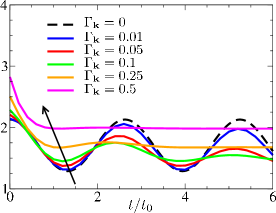
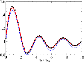
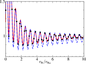
Figure 1: (left) Structure factor at fixed time $t=2t_{0}$ (see text) as a function of momentum $k/k_{0}$, for different values of the damping parameter $\Gamma_{{\bf k}}$, in the case of a quench up with $g_{f}/g_{i}\simeq 1.8$. The arrow indicates the apparent up-shift of the frequency of the oscillations. Bogoliubov theory corresponds to $\Gamma_{{\bf k}}=0$ (black dashed line). (center) Structure factor for quench down at $t=t_{0}$ as a function of $\epsilon_{\bf k}/\epsilon_{{\bf k}_{0}}$ with $\Gamma_{\bf k}=0.01$. The red curve is our result, the blue dashed curve Bogoliubov theory and the symbols a “phenomenological fit” (see text). (right) same as the central figure, but for $t=5t_{0}$.

Out-of-equilibrium correlation functions We now specify the out-of-equilibrium observables we will study. Because our model Hamiltonian is quadratic, it is reasonably straightforward to derive the four correlation functions involving combinations of $\psi$ and $\psi^{\dagger}$. Here we will concentrate on the density-density correlation functions, which are easily accessed in current cold atoms experiments Hung et al. (2011). The density operator is defined in momentum space as $\hat{\rho}_{\bf q}(t)=\sum_{k}\hat{a}^{\dagger}_{{\bf k}+{\bf q}}(t)\hat{a}_{\bf k}(t)$, where $\hat{a}_{\bf k}=\sqrt{n_{0}}\delta_{{\bf k},0}+\hat{\psi}_{\bf k}$. The different correlation functions will involve the usual time ordered normal ($G_{\bf k}(t,s)$) and anomalous ($F_{\bf k}(t,s)$) Green’s functions. Because of the quench, these Green’s functions depend separately on their two time arguments. We find as expected that in the long time limit, when the system reaches its new equilibrium state, they become functions of only $t-s$. This is a non-trivial test of the current theory which reflects the energy dissipation mechanism.

The density-density correlation function $\chi_{\bf q}(t,s)=\langle\hat{\rho}_{\bf q}(t)\hat{\rho}_{-{\bf q}}(s)\rangle-\langle\hat{\rho}_{\bf q}(t)\rangle\langle\hat{\rho}_{-{\bf q}}(s)\rangle$, (with $t\geq s$) is related to the structure factor $S_{\bf q}(t)=\chi_{\bf q}(t,t)/n_{0}$. It can similarly be written in terms of the Green’s functions so that $\chi_{\bf q}(t,s)=-n_{0}\Big{\{}G_{\bf q}(t,s)+G_{\bf q}(s,t)+F_{\bf q}(t,s)+F_{\bf q}^{\dagger}(t,s)\Big{\}}+\sum_{\bf k}\Big{\{}G_{{\bf k}+{\bf q}}(s,t)G_{\bf k}(t,s)+F^{\dagger}_{{\bf k}+{\bf q}}(t,s)F_{\bf k}(t,s)\Big{\}}$, where the sum is over all ${\bf k}$ different from $0$ and $-{\bf q}$. Because the condensate is macroscopically occupied, we will neglect the second term in brackets in our numerical calculation of the structure factor Natu and Mueller (2012); Hung et al. (2012).

It is convenient to define the 4-vector $\Upsilon(t,s)=\Big{\{}F_{\bf k}(t,s),G_{\bf k}(s,t),G_{\bf k}(t,s),F^{\dagger}_{\bf k}(t,s)\Big{\}}$. These component Green’s functions can be evaluated by solving equation (5) which yields ($t>s$)

$$\Upsilon(t,s)=\int_{0}^{t}du\int_{0}^{s}dv{\cal M}_{\bf k}(v)\otimes{\cal M}_{\bf k}(u)\cdot\Upsilon_{i}(t-s-u+v),$$ (7)

where the matrix ${\cal M}_{\bf k}(v)=\int_{0}^{v}M_{\bf k}(v-v^{\prime}).M_{{\bf k},i}^{-1}(v^{\prime})dv^{\prime}$ and $M_{{\bf k},i}^{-1}(t)$ is the inverse of the $M_{\bf k}$ with $g_{f}\to g_{i}$, with the definition $\int_{0}^{v}M_{\bf k}(v-v^{\prime}).M_{{\bf k}}^{-1}(v^{\prime})dv^{\prime}=\delta(v)$. We have introduced the vector $\Upsilon_{i}(t)=\Big{\{}{\cal F}_{{\bf k},i}(t),{\cal G}_{{\bf k},i}(-t),{\cal G}_{{\bf k},i}(t),{\cal F}^{\dagger}_{{\bf k},i}(t)\Big{\}}$, corresponding to the equilibrium Green’s functions of the initial Hamiltonian. These can be defined using the the equilibrium bosonic spectral functions . Our equations correspond to Bogoliubov theory in the absence of a bath.

While Eq. 7 may seem formally complex, the physics it contains needs to be emphasized. Importantly, this equation is consistent with the fluctuation-dissipation theorem. Stated alternatively, it is consistent with the proper asymptotic (long time) regime which requires that the final state of the system be time independent. It can be shown directly from Eq. 7 that the long time limit of $\Upsilon(t+\tau,t)\to\Upsilon_{f}(\tau)$, which means that at long times the proper equilibrium normal and anomalous Green’s function of the quenched Hamiltonian $\hat{H}_{f}$ are obtained. It should not be presumed that one can view this final state as a convolution of a damping term and simple Bogoliubov theory; the asymptote of the structure factor (for example) is finite, as a new equilibrium phase is reached, so that the oscillations are not simply damped out.

Numerical results We discuss now the numerical solution of the previous equations. We introduce the characteristic momentum $k_{0}=\sqrt{n_{0}mg_{i}}$ and time $t_{0}^{-1}=k_{0}^{2}/2m$. Note that $k_{0}$ is the inverse healing length of the condensate at $t=0$. The left panel of Figure 1 shows the evolution in time of the structure factor at a fixed $|{\bf k}|$ after the quench-up for different values of the bath parameter $\Gamma_{\bf k}$ chosen to be independent of $|{\bf k}|$ for simplicity. We also plot the results from Bogoliubov theory which corresponds to the case $\Gamma_{\bf k}=0$. Here we stress that because of damping there is no single frequency observed for each $\mathbf{k}$. Nevertheless, an important effect of the bath (indicated by the arrow) is the shift toward earlier time of the first extrema of the oscillations, leading to an apparent frequency increase. This shift was observed in Hung et al. (2012) for a quench-up (where the effect of the bath is expected to be more important in the dynamics) and cannot be explained by Bogoliubov theory. This effect was not seen for a quench-down, which might be expected, as in this case $\Gamma_{\bf k}$ is smaller.

The central and right panels of Figure 1 plot $S_{\bf k}(t)$ at fixed time $t=t_{0}$ and $t=10t_{0}$ for small $\Gamma=0.01$ in our theory as compared with Bogoliubov theory. For the latter, at long time one sees that $S_{\bf k}(t)$ oscillates faster and faster while never reaching a new equilibrium. We find a moderately successful phenomenological fit to our calculations at low damping with $S^{ph}_{\bf k}(t)=S_{{\bf k},f}+f_{\bf k}(t)\Big{(}\big{[}1+(E^{2}_{{\bf k},i}-E^{2}_{{\bf k},f})/(E_{{\bf k},f})\sin(E_{{\bf k},f}t)^{2}\big{]}S_{{\bf k},i}-S_{{\bf k},f}\Big{)}$, where $S_{{\bf k},i}$ ($S_{{\bf k},f}$) is the initial (final) equilibrium structure factor. For $|{\bf k}|\gg g_{f}n_{0}$, we observe from our theory that $f_{\bf k}(t)=\exp(-(|{\bf k}|/K(t))^{2})$, where $K(t)=k_{0}\sqrt{\frac{(1+\Gamma_{\bf k}^{2})t_{0}}{\Gamma_{\bf k}t}}$. Fits to our theory are shown in the central and right panels of Figure 1. It should be stressed that for these small values of the damping, as illustrated here, there is not yet a signature of an apparent shift in frequency.

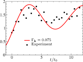
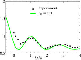
Figure 2: Structure factor at fixed momentum as function of time. (left) quench down $g_{f}/g_{i}\simeq 0.3$ and $k=0.9/\mu m$ with $k_{0}=1.6/\mu m$ and $t_{0}=0.7ms$. (right) quench up $g_{f}/g_{i}\simeq 2.4$ and $k=1.2/\mu m$ with $k_{0}=1/\mu m$ and $t_{0}=2ms$.

Experimental results We have reported Hung et al. (2012) the experimental observation of oscillatory behavior of the density structure factor associated with a sudden quench in a 2D Bose system in the almost-pure- superfluid phase of a cesium atomic gas. The emphasis of the present paper is on damping effects we observe in these oscillations. These are in contrast to an extensive literature focusing on shortcuts to adiabaticity after a fast change of the experimental parameters, in particular of 1D gases, (see for instance Torrontegui et al. (2012)).

The data points in Figures 2 represent the measured equal-time structure factor as a function of time at fixed $|{\bf k}|=0.9\mu m^{-1}$ for the final interaction strength $g_{f}=0.19$ and for a quench up with $g_{f}/g_{i}\simeq 2.4$ (Fig. 2b) and a quench down (Fig. 2a) with $|{\bf k}|=1.2\mu m^{-1}$ and $g_{f}/g_{i}\simeq 0.3$. Importantly, in contrast to other experimental studies and deliberate quench protocols Schaff et al. (2011), dissipation is evident and Sakharov oscillations will eventually be damped out in the steady state. We do not address this asymptotic long time regime because our focus is on reasonably short times where the trap geometry is not important.

We plot as solid lines in Figure 2, theoretical curves with the same microscopic parameters. The color-coded curves represent the regime of moderate damping for different values of $\Gamma=0.1$ (in a quench up) and $\Gamma=0.075$ (in a quench down). Since our focus is on semi-quantitative comparisons, we have allowed a global shift of the y-axis as well as the x-axis (to take care of time uncertainties on the order of $\lesssim 1ms$, due to time lapse between the quench and the detection).

In overall comparison between theory and experiment we find that $\Gamma_{\mathbf{k}}\approx 0.1$ describes the current data set. From this observation, one cannot yet characterize the microscopic nature and origin of dissipation, but our work should be viewed as a first step in the process. Additional experiments and more systematic comparisons can be anticipated in future. Nevertheless, with this approach, we can, however, address several features of the experiments which were difficult to understand within strict Bogoliubov theory such as the apparent frequency shifts and the damping both in time and $\mathbf{k}$. A general theme of this paper has been to focus on damping effects. Nevertheless, our out of equilibrium studies necessarily have implications on the equilibrium behavior (of the structure factor, say) due to the important fluctuation-dissipation relation. In summary, in this paper we have demonstrated that the introduction of a Leggett-Caldeira bath for a Bose superfluid implies that the dynamics can be derived exactly and the calculations of the response functions such as the structure factors is then precise and fully consistent.

A.R. thanks J. Bonart for discussions. This work is supported by NSF-MRSEC Grant 0820054. C.L. and C.C. acknowledge support from NSF Grant No. PHY-0747907 and under ARO Grant No. W911NF0710576 with funds from the DARPA OLE Program.

References

- Donley et al. (2001) E. A. Donley, N. R. Claussen, S. L. Cornish, J. L. Roberts, E. A. Cornell, and C. E. Wieman, Nature, 412, 295 (2001).
- Greiner et al. (2005) M. Greiner, C. A. Regal, and D. S. Jin, Phys. Rev. Lett., 94, 070403 (2005).
- Caldeira and Leggett (1983) A. Caldeira and A. Leggett, Physica A: Statistical Mechanics and its Applications, 121, 587 (1983).
- Ford and Kac (1987) G. W. Ford and M. Kac, Journal of Statistical Physics, 46, 803 (1987), 10.1007/BF01011142.
- Grabert et al. (1988) H. Grabert, P. Schramm, and G.-L. Ingold, Physics Reports, 168, 115 (1988), ISSN 0370-1573.
- Bonart and Cugliandolo (2013) J. Bonart and L. F. Cugliandolo, EPL (Europhysics Letters), 101, 16003 (2013).
- Bonart and Cugliandolo (2012) J. Bonart and L. F. Cugliandolo, Phys. Rev. A, 86, 023636 (2012).
- Chang and Chakravarty (1985) L.-D. Chang and S. Chakravarty, Phys. Rev. B, 31, 154 (1985).
- Hung et al. (2012) C.-L. Hung, V. Gurarie, and C. Chin, ArXiv e-prints (2012), arXiv:1209.0011 [cond-mat.quant-gas] .
- Tan and Levin (2004) S. Tan and K. Levin, Phys. Rev. B, 69, 064510 (2004).
- Natu and Mueller (2012) S. S. Natu and E. J. Mueller, ArXiv e-prints (2012), arXiv:1207.4509 [cond-mat.quant-gas] .
- Ullah and Dorsey (1990) S. Ullah and A. T. Dorsey, Phys. Rev. Lett., 65, 2066 (1990).
- Blakie et al. (2008) P. Blakie, A. Bradley, M. Davis, R. Ballagh, and C. Gardiner, Advances in Physics, 57, 363 (2008).
- Stoof (1997) H. T. C. Stoof, Phys. Rev. Lett., 78, 768 (1997).
- (15) S. P. Cockburn and N. P. Proukakis, arXiv e-print /1207.1216.
- Beliaev (1958) S. T. Beliaev, Sov. Phys. JETP, 7, 289 (1958a), zh. Eksp. Teor. Fiz. 34, 417 (1958).
- Beliaev (1958) S. T. Beliaev, Sov. Phys. JETP, 7, 299 (1958b), zh. Eksp. Teor. Fiz. 34, 433 (1958).
- Hung et al. (2011) C.-L. Hung, X. Zhang, L.-C. Ha, S.-K. Tung, N. Gemelke, and C. Chin, New Journal of Physics, 13, 075019 (2011).
-
Note (1)
The spectral function and its anomalous counterpart are given in terms of the Green’s function
with the self-energy , by
(10)
where . Note that the spectrum is gapless, as and that has the sign of as required for bosons. In order to respect the commutation relation at equal time, we have and .(11) - Torrontegui et al. (2012) E. Torrontegui, S. Ibáñez, S. Martí nez Garaot, M. Modugno, A. del Campo, D. Guéry-Odelin, A. Ruschhaupt, X. Chen, and J. G. Muga, ArXiv e-prints (2012), arXiv:1212.6343 [quant-ph] .
- Schaff et al. (2011) J.-F. Schaff, P. Capuzzi, G. Labeyrie, and P. Vignolo, New Journal of Physics, 13, 113017 (2011).