Certifying The Quantumness of A Generalized Coherent Control Scenario

Abstract

We consider the role of quantum mechanics in a specific coherent control scenario, designing a “coherent control interferometer” as the essential tool that links coherent control to quantum fundamentals. Building upon this allows us to rigorously display the genuinely quantum nature of a generalized weak-field coherent control scenario (utilizing 1 vs. 2 photon excitation) via a Bell-CHSH test. Specifically, we propose an implementation of “quantum delayed-choice” in a bichromatic alkali atom photoionization experiment. The experimenter can choose between two complementary situations, which are characterized by a random photoelectron spin polarization with particle-like behavior on the one hand, and by spin controllability and wave-like nature on the other. Because these two choices are conditioned coherently on states of the driving fields, it becomes physically unknowable, prior to measurement, whether there is control over the spin or not.

I Introduction

Various coherent control scenarios, in both complex and simple systems, utilize laser fields to coherently manipulate atomic or molecular fragmentation processes Shapiro and Brumer (2012a). Two competing, fundamentally different perspectives have been advocated to explain the control. In the first, within the spirit of the Young double-slit experiment, one interprets the probability of the outcomes—the control target or yield—as an intensity and phase dependent pattern resulting from the quantum-coherent interference of mutually exclusive path alternatives that are embodied in the laser excitation pathways Rice and Zhao (2000); Shapiro and Brumer (2012b, a). In the second, one views the controllability as the manifestation of the response of the system to the superposition of phase-coherent incident laser fields. In this approach, control is perceived as an inherently classical phenomenon Constantoudis and Nicolaides (2005); de Lima and de Aguiar (2008); Ivanov, Bartram, and Smirnova (2012), i.e. a phenomenon that could fall under descriptions based on classical laws of motion. Understanding which of these descriptions is preferred is not just a matter of convenience. Rather, it has practical applications stemming from the recognition that decoherence effects often bring a system to the classical limit Schlosshauer (2007). Hence, if control is indeed (at least partially) classical, then it may well survive in the often unavoidable decohering environments associated with realistic molecular processes.

There is ample motivation to address the issue of the role of quantum vs. classical effects in coherent control. For example, Refs. 8 and 9 analyze controlled symmetry breaking in a field-driven quartic oscillator both quantum-mechanically and classically and concludes that not only the basic requirements, but also the physical origins of control, are the same in both cases. Similarly, Ref. 10 shows that environmentally assisted one photon phase control is mainly due to the incoherent breaking of time-reversal symmetry, and is thereby not evidence of quantum coherent dynamics. In addition, it is of interest to note that related concerns regarding classical vs. quantum coherence contributions have arisen within the framework of electronic energy transfer in light-harvesting systems Miller (2012).

Classical descriptions can offer an intuitively appealing picture, but in the case of coherent control they often fail quantitatively, and are hence discarded. Therefore, since its inception, coherent control has been regarded as fundamentally quantum Brumer and Shapiro (1986); Shapiro, Hepburn, and Brumer (1988); Shapiro and Brumer (2012a), particularly in the case of driving a system with two frequencies $(n\omega+m\omega)$. Here, reliance on an interpretation of the interference of quantum pathways as described above (and as originally put forth Brumer and Shapiro (1986); Shapiro, Hepburn, and Brumer (1988) by one of the authors of this paper) is commonly accepted. But the issue of the extent to which nontrivial quantum features are central to phenomena such as coherent control needs to be reconsidered in light of developments in Bell-like tests to certify unique quantum features Bell (1964, 1966); Clauser et al. (1969); Gühne and Tóth (2009); Ionicioiu and Terno (2011); Peruzzo et al. (2012); Kaiser et al. (2012) and recent reports that identify distinct classical mechanisms as a possible source of control Flach, Yevtushenko, and Zolotaryuk (2000); Sirko and Koch (2002); Franco and Brumer (2006, 2008); de Lima and de Aguiar (2008); Franco, Spanner, and Brumer (2010); Pachon and Brumer (2013).

We reiterate that there is no question that quantum mechanics is necessary to quantitatively describe the outcome of coherent control scenarios. However, quantitative agreement with a quantum description cannot serve as a general proof that the observed phenomenon is unambiguously quantum in nature (since such a proof requires that all classical descriptions and explanations must be falsified). As a consequence, rigorously certifying the quantumness of a process and identifying its quantum features is a challenging task that has been the subject of intense efforts in quantum optics, quantum information and quantum foundations. Studies of this type often take the form of proposed experimental protocols that are carefully crafted to close any loopholes that would prevent rigorous assertions regarding those features of quantum mechanics that are manifest in the process. Such features include issues such as nonlocality, entanglement, multiple-pathway interference, sensitivity to measurement, etc. Greenstein and Zajonc (2005). In this paper we make the first inroads into utilizing ideas of this kind to explore the quantum characteristics of coherent control. Specifically, we first focus on path interference and introduce a “coherent control interferometer” which formalizes the relationship between coherent control scenarios and quantum optics approaches to the fundamentals of quantum mechanics Greenstein and Zajonc (2005); Haroche and J-M (2006). As a particular case we concentrate the analysis on phase-coherent control over the spin polarization of an electron that has been emitted in an interfering $(\omega+2\omega)$ photoionization process.

We then design a generalized coherent control scenario in which measurements can be performed whose outcomes will have certifiably nonclassical statistics and that strongly support the analogy between coherent control and the quantum interference of paths. We show that this setup can be used to probe wave-particle complementarity and to implement “quantum delayed-choice” Ionicioiu and Terno (2011); Peruzzo et al. (2012); Kaiser et al. (2012); it becomes unforeseeable prior to measurement whether the spin polarization statistics are wave- or particle-like, that is, whether there is control or not. This hallmark of quantum interference is key for violating a Bell inequality that serves as a rigorous experimental test of local realism and thereby distinguishes nonclassical from classical statistics, entirely on the basis of observed statistical data Bell (1964, 1966); Clauser et al. (1969); Gühne and Tóth (2009).

Note the fact that we deal with a generalization of traditional coherent control scenarios indicates the continuing need to identify methods of certifying the quantumness of traditional coherent control scenarios. Such studies are underway and our expectation is that the coherent control interferometer introduced in this paper will serve as a central tool for such studies.

II Control Scenario

II.1 Coherent Control Interferometer

Let a heavy alkali atom be ionized by weak coherent ($\omega+2\omega$) radiation Yin et al. (1992); Yin and Elliott (1993); Wang and Elliott (2001). For purposes of simplification (rather than physical necessity), we assume a tight confinement that fully suppresses decoherence due to recoil . The control target is the laboratory $\hat{\boldsymbol{z}}\vphantom{\boldsymbol{z}}$-axis projection $m_{s}^{\prime}$ of the photoelectron’s spin in the continuum Fano (1969); Baum, Lubell, and Raith (1970). We consider the case where the continuum state $\mathopen{}\mathclose{{}\left|\boldsymbol{K}^{\prime},m_{s}^{\prime}{}^{+}}\right\rangle$ of the electron at energy $E^{\prime}=\mathopen{}\mathclose{{}\left(\hbar K^{\prime}}\right){}^{2}/2m_{e}$ can be reached from the atomic ground state $\mathopen{}\mathclose{{}\left|n\mathrm{S}\frac{1}{2},m_{j}}\right\rangle$ mainly by two pathways Taylor (1972): (i) absorption of $1$ photon of energy $\hbar\omega_{2}=E^{\prime}-E\mathopen{}\mathclose{{}\left(n\mathrm{S}\frac{1}{2}}\right)$ or (ii) of $2$ photons each with energy $\hbar\omega_{1}=\hbar\omega_{2}/2$. Here, $\boldsymbol{K}^{\prime}$ refers to the electron’s asymptotic outgoing wavevector Taylor (1972), $n$ is the ground state’s principle quantum number Bethe and Salpeter (2008), and the projection of the total angular momentum $j$ onto the $\hat{\boldsymbol{z}}\vphantom{\boldsymbol{z}}$-axis is denoted $m_{j}$. This setup implements a “coherent control interferometer” (CCI), Fig. 1, an analog of a Mach-Zehnder interferometer (MZI). The ground state is spin-$\frac{1}{2}$ and constitutes the CCI’s two input ports whereas the final projections $m_{s}^{\prime}=\pm\frac{1}{2}$ are identified with the two output ports, the measurement statistics $p_{\pm}$ of which are interpreted as the interference patterns. Henceforth, we restrict attention to one input port only, $m_{j}=-\frac{1}{2}$.

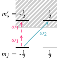
(a)        (b)  

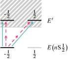
Figure 1: (color online) Proposed coherent control interferometer (CCI). (a) In the open configuration $o$, single-photon ionization (solid blue) only undergoes a $\sigma$-transition with $\big{\lvert}m_{j}-m_{s}^{\prime}\big{\rvert}=1$, whereas two-photon ionization (dashed red) leaves the electron spin unchanged. The processes are distinguishable from one another due to their different outcomes. (b) This is not the case in the closed setup $c$, for which the transition amplitudes between all spin combinations are nonzero.

The incoming laser modes $l$ are to be populated with coherent states of light, $|l\rangle\equiv\mathopen{}\mathclose{{}\left|\mathopen{}\mathclose{{}\left(\alpha\boldsymbol{k}\hat{\boldsymbol{\varepsilon}}\vphantom{\boldsymbol{\varepsilon}}}\right)_{l}}\right\rangle$, since these are eigenstates of the photon annihilation operator and thus correlations with matter due to photon absorption do not occur Gong and Brumer (2010). The a priori probabilities of the ionization pathways can be adjusted by means of the amplitude moduli $\mathopen{}\mathclose{{}\left\lvert\alpha_{l}}\right\rvert$, the directions of incidence $\boldsymbol{k}_{l}$, and the polarizations $\hat{\boldsymbol{\varepsilon}}\vphantom{\boldsymbol{\varepsilon}}_{l}$. This is because (as described in the appendix), in the long-time limit, the change of the electron’s spin is described in terms of an infinite series of well-known, polarization-dependent transition matrix amplitudes $t_{i}\bigl{(}m_{s}^{\prime},m_{j}^{\vphantom{\prime}}\bigr{)}$, $i=1,2,\ldots$, multiplied by corresponding powers of the field amplitudes $\alpha_{l}$ Cohen-Tannoudji, Dupont-Roc, and Grynberg (1998); Fermi (1930); Seaton (1951); Cooper (1962); Burgess and Seaton (1960); Bebb (1966); Lambropoulos and Teague (1976). In the present case, only the first two transition amplitudes are relevant Yin et al. (1992); Yin and Elliott (1993); $t_{1}$ resolves the $1$-photon process and connects only to $\mathrm{P}$ continuum states, whereas $t_{2}$ accounts for $2$-photon ionization and accesses $\mathrm{S}$ and $\mathrm{D}$ orbitals. The amplitudes contain radial integrals, $D_{1}$ and $D_{2}$, that serve here as complex empirical parameters. There exist measurement schemes for which the ionization pathways become absolutely distinguishable. Therefore, in what follows, spin statistics are conditioned on successful detection of the electron in the channel $\hat{\boldsymbol{K}}\vphantom{\boldsymbol{K}}^{\prime}=\bigl{(}\sqrt{2}\,\hat{\boldsymbol{x}}\vphantom{\boldsymbol{x}}-\hat{\boldsymbol{z}}\vphantom{\boldsymbol{z}}\bigr{)}/\sqrt{3}$. This both eliminates the need for taking into account the efficiency of detection and does not provide information about the path taken from the initial to final state of the atom.

Figure 2: (color online) Sample scattering geometry with incident light wavevectors $\hat{\boldsymbol{k}}\vphantom{\boldsymbol{k}}_{1o}=\hat{\boldsymbol{y}}\vphantom{\boldsymbol{y}}$, $\hat{\boldsymbol{k}}\vphantom{\boldsymbol{k}}_{2o}$ with projection $\hat{\boldsymbol{k}}\vphantom{\boldsymbol{k}}_{2o}\cdot\hat{\boldsymbol{z}}\vphantom{\boldsymbol{z}}=\cos\vartheta_{2o}=-\sqrt{2/3}$, $\hat{\boldsymbol{k}}\vphantom{\boldsymbol{k}}_{1c}=\hat{\boldsymbol{K}}\vphantom{\boldsymbol{K}}^{\prime}$, and $\hat{\boldsymbol{k}}\vphantom{\boldsymbol{k}}_{2c}$ with $\cos\vartheta_{2c}=-2\sqrt{2}/3$. The emitted photoelectron is detected in the direction $\hat{\boldsymbol{K}}\vphantom{\boldsymbol{K}}^{\prime}$. The alkali atom is located at the origin. The polarization of the incoming radiation is indicated in color (shades of grey). The $o$ configuration uses linear polarization, whereas the $c$ setup employs elliptically polarized light.

We argue that quantum interference in the CCI can be exposed in the same manner as it can be displayed in the Young double-slit Scully, Englert, and Walther (1991); Itano et al. (1998), a MZI, or a Ramsey interferometer Englert (1996); Bertet et al. (2001) for single photons, electrons, etc. The latter undertaking entails the observation of complementarity between the wave and particle property, which is demonstrated by the experimenter’s choice between two measurement statistics: particle and wave statistics. In the case of the former, interference is completely absent. In principle, if not in practice, knowledge about the path—whether the photon has taken the first rather than the second slit, or, correspondingly, whether the atom has been ionized in a $1$- or a $2$-photon process—is available by measurement. When it allows for tracing of paths, an interferometer is called open. If, in contrast, interference is displayed, then the statistics are wave-like. Full path knowledge cannot be acquired, not even in principle. This results from operating the interferometer in the so-called closed configuration. Below, the subscripts $o$ and $c$ are used to denote these configurations.

The ionization scenario has been selected because it is conducive to engineering both the $o$ and $c$ cases, Fig. 2.

II.1.1 The Open Interferometer Configuration

For the open configuration, two linearly polarized modes, $\mathopen{}\mathclose{{}\left(\boldsymbol{k}\hat{\boldsymbol{\varepsilon}}\vphantom{\boldsymbol{\varepsilon}}}\right)_{1o}$ and $\mathopen{}\mathclose{{}\left(\boldsymbol{k}\hat{\boldsymbol{\varepsilon}}\vphantom{\boldsymbol{\varepsilon}}}\right)_{2o}$, are chosen, for example, to be populated according to $\hat{\boldsymbol{\varepsilon}}\vphantom{\boldsymbol{\varepsilon}}_{1o}=-\hat{\boldsymbol{k}}\vphantom{\boldsymbol{k}}_{2o}=\bigl{(}\hat{\boldsymbol{x}}\vphantom{\boldsymbol{x}}+\sqrt{2}\,\hat{\boldsymbol{z}}\vphantom{\boldsymbol{z}}\bigr{)}/\sqrt{3}$ and $\hat{\boldsymbol{\varepsilon}}\vphantom{\boldsymbol{\varepsilon}}_{2o}=\hat{\boldsymbol{k}}\vphantom{\boldsymbol{k}}_{1o}=\hat{\boldsymbol{y}}\vphantom{\boldsymbol{y}}$ in a field state denoted $\mathopen{}\mathclose{{}\left|1o,2o}\right\rangle$. The vectors $\hat{\boldsymbol{K}}\vphantom{\boldsymbol{K}}^{\prime}$, $\hat{\boldsymbol{k}}\vphantom{\boldsymbol{k}}_{2o}$, and $\hat{\boldsymbol{k}}\vphantom{\boldsymbol{k}}_{1o}$ come as a right-handed orthogonal triad that is inclined at an angle $\pi-\arctan(\sqrt{2})$ away from the positive $\hat{\boldsymbol{z}}\vphantom{\boldsymbol{z}}$-axis. These mode settings imply $t_{1o}\propto\delta_{m_{s}^{\prime},-m_{j}}$ and $t_{2o}\propto\delta_{m_{s}^{\prime},m_{j}}$ and, as a result, absolute path knowledge; the direction in which the spin is detected reveals the path taken through the CCI, cf. Figs. 1 (a) and 2. To realize an unbiased interferometer, the moduli of the complex amplitudes are to be adjusted as follows:

$$\mathopen{}\mathclose{{}\left\lvert\alpha_{1o}}\right\rvert =\frac{6\sqrt{\pi}\lambda\mathrm{e}^{\mathrm{i}\kappa_{1o}}}{\hbar g_{k_{1}}\mathopen{}\mathclose{{}\left[-D_{1}\mathopen{}\mathclose{{}\left(E^{\prime}\mathrm{P}\tfrac{1}{2},n\mathrm{S}\tfrac{1}{2}}\right)+D_{1}\mathopen{}\mathclose{{}\left(E^{\prime}\mathrm{P}\tfrac{3}{2},n\mathrm{S}\tfrac{1}{2}}\right)}\right]},$$ (1a)

$$\mathopen{}\mathclose{{}\left\lvert\alpha_{2o}}\right\rvert^{2} =\frac{90\sqrt{\pi}\lambda\mathrm{e}^{\mathrm{i}\kappa_{2o}}}{\mathrm{i}\hbar_{\vphantom{k_{2}}}^{2}g_{k_{2}}^{2}}\bigl{[}-5D_{2}\mathopen{}\mathclose{{}\left(E^{\prime}\mathrm{S}\tfrac{1}{2},\mathrm{P}\tfrac{1}{2},n\mathrm{S}\tfrac{1}{2}}\right)$$

$$-10D_{2}\mathopen{}\mathclose{{}\left(E^{\prime}\mathrm{S}\tfrac{1}{2},\mathrm{P}\tfrac{3}{2},n\mathrm{S}\tfrac{1}{2}}\right)+5D_{2}\mathopen{}\mathclose{{}\left(E^{\prime}\mathrm{D}\tfrac{3}{2},\mathrm{P}\tfrac{1}{2},n\mathrm{S}\tfrac{1}{2}}\right)$$

$$+D_{2}\mathopen{}\mathclose{{}\left(E^{\prime}\mathrm{D}\tfrac{3}{2},\mathrm{P}\tfrac{3}{2},n\mathrm{S}\tfrac{1}{2}}\right)+9D_{2}\mathopen{}\mathclose{{}\left(E^{\prime}\mathrm{D}\tfrac{5}{2},\mathrm{P}\tfrac{3}{2},n\mathrm{S}\tfrac{1}{2}}\right)\bigr{]}^{-1}.$$ (1b)

The Eqs. (1) define conditions on the phases $\kappa_{1o}$ and $\kappa_{2o}$ that ensure that the right hand sides of Eq. (1a) and (1b) are real and nonnegative. $\kappa_{1o}$ and $\kappa_{2o}$ therefore depend on the complex phases of the integrals $D_{1}$ and $D_{2}$ and will henceforth be referred to as material phases. The arguments of $D_{1}$ and $D_{2}$ refer to the respective photoionization channels. For example, $D_{2}\mathopen{}\mathclose{{}\left(E^{\prime}\mathrm{D}\tfrac{5}{2},\mathrm{P}\tfrac{3}{2},n\mathrm{S}\tfrac{1}{2}}\right)$ is the radial matrix element of the process leading from the ground state $\big{|}n\mathrm{S}\tfrac{1}{2},m_{j}^{\vphantom{\prime}}\big{\rangle}$ via intermediate $\mathrm{P}\tfrac{3}{2}$ orbitals to the continuum state $\big{|}E^{\prime}\mathrm{D}\tfrac{5}{2},m_{j}^{\prime}{}^{+}\big{\rangle}$. The field’s phases, $\phi_{1o}=\operatorname{Arg}\alpha_{1o}$ and $\phi_{2o}=\operatorname{Arg}\alpha_{2o}$, can still be chosen freely. In Eqs. (1), $\lambda$ is a positive, constant scaling factor. The precise value of $\lambda$ is irrelevant, since the probability amplitudes are eventually conditioned on successful detection of the photoelectron in the channel $\hat{\boldsymbol{K}}\vphantom{\boldsymbol{K}}^{\prime}$. For the choices above, $\mathopen{}\mathclose{{}\left\lvert t_{1o}^{\vphantom{2}}\alpha_{1o}^{\vphantom{2}}}\right\rvert=\mathopen{}\mathclose{{}\left\lvert t_{2o}^{\vphantom{2}}\alpha_{2o}^{2}}\right\rvert$. We have thus established that, for the initial state $\mathopen{}\mathclose{{}\left|n\mathrm{S}\tfrac{1}{2},\text{-}\tfrac{1}{2}}\right\rangle\otimes\mathopen{}\mathclose{{}\left|1o,2o}\right\rangle$, the final state of the ionized atom in the channel $\boldsymbol{K}^{\prime}$ is $\mathopen{}\mathclose{{}\left|f_{o}}\right\rangle\otimes\mathopen{}\mathclose{{}\left|1o,2o}\right\rangle$, where

$$\mathopen{}\mathclose{{}\left|f_{o}}\right\rangle =\frac{\mathrm{e}^{\mathrm{i}\delta_{o}}}{\sqrt{2}}\,\mathopen{}\mathclose{{}\left(\mathopen{}\mathclose{{}\left|\boldsymbol{K}^{\prime},\tfrac{1}{2}{}^{+}}\right\rangle+\mathrm{e}^{-\mathrm{i}\theta_{o}}\mathopen{}\mathclose{{}\left|\boldsymbol{K}^{\prime},\text{-}\tfrac{1}{2}{}^{+}}\right\rangle}\right)$$ (2)

with $\delta_{o}=\phi_{1o}+\kappa_{1o}$ and $\theta_{o}=\phi_{1o}-2\phi_{2o}+\kappa_{1o}-\kappa_{2o}$. The state $\mathopen{}\mathclose{{}\left|f_{o}}\right\rangle$ describes full particle-like statistics; projected onto the $\hat{\boldsymbol{z}}\vphantom{\boldsymbol{z}}$ axis, both spin orientations $m_{s}^{\prime}=\pm\frac{1}{2}$ are always equally likely, regardless of the lasers’ phase difference $\phi_{1o}-2\phi_{2o}$. Thus there is no phase-coherent control and the fringe visibility vanishes on both output ports.

II.1.2 The Closed Interferometer Configuration

As for the closed configuration $c$, it can be achieved by populating two other modes, $\mathopen{}\mathclose{{}\left(\boldsymbol{k}\hat{\boldsymbol{\varepsilon}}\vphantom{\boldsymbol{\varepsilon}}}\right)_{1c}$ and $\mathopen{}\mathclose{{}\left(\boldsymbol{k}\hat{\boldsymbol{\varepsilon}}\vphantom{\boldsymbol{\varepsilon}}}\right)_{2c}$ (see Fig. 2). For example, the one-photon absorption field $1c$ is chosen circularly polarized, $\sqrt{14}\,\hat{\boldsymbol{\varepsilon}}\vphantom{\boldsymbol{\varepsilon}}_{1c}=\sqrt{5\smash{/}3+\sqrt{2}}\,\bigl{(}\hat{\boldsymbol{x}}\vphantom{\boldsymbol{x}}+\sqrt{2}\,\hat{\boldsymbol{z}}\vphantom{\boldsymbol{z}}\bigr{)}-\mathrm{i}\sqrt{9-3\sqrt{2}}\,\hat{\boldsymbol{y}}\vphantom{\boldsymbol{y}}$ with $\hat{\boldsymbol{k}}\vphantom{\boldsymbol{k}}_{1c}=\hat{\boldsymbol{K}}\vphantom{\boldsymbol{K}}^{\prime}$, whereas the two-photon absorption field $2c$ is chosen elliptically polarized, $\sqrt{2}\,\hat{\boldsymbol{\varepsilon}}\vphantom{\boldsymbol{\varepsilon}}_{2c}=\bigl{(}2\sqrt{2}\,\hat{\boldsymbol{x}}\vphantom{\boldsymbol{x}}+\hat{\boldsymbol{z}}\vphantom{\boldsymbol{z}}\bigr{)}/3+\mathrm{i}\hat{\boldsymbol{y}}\vphantom{\boldsymbol{y}}$ as well as $\hat{\boldsymbol{k}}\vphantom{\boldsymbol{k}}_{2c}=\bigl{(}\hat{\boldsymbol{x}}\vphantom{\boldsymbol{x}}-2\sqrt{2}\,\hat{\boldsymbol{z}}\vphantom{\boldsymbol{z}}\bigr{)}/3$, making an angle of $\pi-\operatorname{arccsc}(3)$ with the $\hat{\boldsymbol{z}}\vphantom{\boldsymbol{z}}$-axis. The resultant field state is denoted $\mathopen{}\mathclose{{}\left|1c,2c}\right\rangle$. Only $t_{2}\mathopen{}\mathclose{{}\left(\tfrac{1}{2},\tfrac{1}{2}}\right)$ and $t_{2}\mathopen{}\mathclose{{}\left(\text{-}\tfrac{1}{2},\text{-}\tfrac{1}{2}}\right)$ contain $\mathrm{S}$-wave $D_{2}$ factors. They are fully suppressed in the chosen field configuration. (It turns out that simultaneous unbiased interference for both input ports of the CCI, $m_{j}=\pm\frac{1}{2}$, cannot be achieved. That is why the above settings are tailored specifically to balance the interference from the input port $m_{j}=-\frac{1}{2}$). With these, we find $t_{1c}\mathopen{}\mathclose{{}\left(\tfrac{1}{2},\text{-}\tfrac{1}{2}}\right)=t_{1c}\mathopen{}\mathclose{{}\left(\text{-}\tfrac{1}{2},\text{-}\tfrac{1}{2}}\right)$. Although it would be most desirable to also have $t_{2c}\mathopen{}\mathclose{{}\left(\tfrac{1}{2},\text{-}\tfrac{1}{2}}\right)=-t_{2c}\mathopen{}\mathclose{{}\left(\text{-}\tfrac{1}{2},\text{-}\tfrac{1}{2}}\right)$, the latter amplitudes are somewhat biased and have generally a mutual phase shift different from $\pi$. This is the case unless one can select an energy $E^{\prime}$ for which the transition to $j^{\prime}=\frac{5}{2}$ is negligible compared to $j^{\prime}=\frac{3}{2}$; indeed, for $D_{2}\mathopen{}\mathclose{{}\left(E^{\prime}\mathrm{D}\tfrac{5}{2},\mathrm{P}\tfrac{3}{2},n\mathrm{S}\tfrac{1}{2}}\right)=0$, the $t_{2c}$ are as desired. If this were the case the amplitudes would be set equal in absolute value to

$$\mathopen{}\mathclose{{}\left\lvert\alpha_{1c}}\right\rvert =\sqrt{\tfrac{7}{2\mathopen{}\mathclose{{}\left(3-\sqrt{2}}\right)}}\,\mathopen{}\mathclose{{}\left\lvert\alpha_{1o}}\right\rvert,$$ (3a)

$$\mathopen{}\mathclose{{}\left\lvert\alpha_{2c}}\right\rvert^{2} =\frac{180\sqrt{\pi}\lambda\mathrm{e}^{\mathrm{i}\kappa_{2c}}}{\mathrm{i}\bigl{(}\sqrt{2}+2\bigr{)}\hbar^{2}g_{k_{2}}^{2}}\bigl{[}5D_{2}\mathopen{}\mathclose{{}\left(E^{\prime}\mathrm{D}\tfrac{3}{2},\mathrm{P}\tfrac{1}{2},n\mathrm{S}\tfrac{1}{2}}\right)$$

$$+D_{2}\mathopen{}\mathclose{{}\left(E^{\prime}\mathrm{D}\tfrac{3}{2},\mathrm{P}\tfrac{3}{2},n\mathrm{S}\tfrac{1}{2}}\right)\bigr{]}^{-1}$$ (3b)

in order to achieve unbiased interference. We choose the amplitudes (3) even for cases where $D_{2}\mathopen{}\mathclose{{}\left(E^{\prime}\mathrm{D}\tfrac{5}{2},\mathrm{P}\tfrac{3}{2},n\mathrm{S}\tfrac{1}{2}}\right)\neq 0$. The phases $\phi_{1c}=\operatorname{Arg}\alpha_{1o}$ and $\phi_{2c}=\operatorname{Arg}\alpha_{2o}$ are free parameters, whereas $\kappa_{2c}$ is another constant material phase that is implicitly defined by Eq. (3b). The phases picked up by the one-photon processes are identical in the configurations $o$ and $c$, therefore $\kappa_{1c}=\kappa_{1o}$. Consider now initialization from the state $\mathopen{}\mathclose{{}\left|n\mathrm{S}\tfrac{1}{2},\text{-}\tfrac{1}{2}}\right\rangle\otimes\mathopen{}\mathclose{{}\left|1c,2c}\right\rangle$. For successful detection in the channel $\boldsymbol{K}^{\prime}$, the final state becomes $\mathopen{}\mathclose{{}\left|f_{c}}\right\rangle\otimes\mathopen{}\mathclose{{}\left|1c,2c}\right\rangle$, where

$$\mathopen{}\mathclose{{}\left|f_{c}}\right\rangle =\frac{\mathrm{e}^{\mathrm{i}\delta_{c}}}{N_{f_{c}}}\,\Bigl{[}\mathopen{}\mathclose{{}\left(\mathrm{i}\sin\tfrac{\phi_{c}+\theta_{c}}{2}-\mathrm{e}^{-\mathrm{i}\phi_{c}/2}d_{2}}\right)\mathopen{}\mathclose{{}\left|\boldsymbol{K}^{\prime},\tfrac{1}{2}{}^{+}}\right\rangle$$

$$+\mathopen{}\mathclose{{}\left(\cos\tfrac{\phi_{c}+\theta_{c}}{2}+\mathopen{}\mathclose{{}\left(\tfrac{7}{2}-\tfrac{5}{\sqrt{2}}}\right)\mathrm{e}^{-\mathrm{i}\phi_{c}/2}d_{2}}\right)\mathopen{}\mathclose{{}\left|\boldsymbol{K}^{\prime},\text{-}\tfrac{1}{2}{}^{+}}\right\rangle\Bigr{]}$$ (4)

with the global phase $\delta_{c}=\mathopen{}\mathclose{{}\left(\phi_{1c}+2\phi_{2c}+\kappa_{1c}+\kappa_{2c}}\right)/2$, the interferometric phase difference $\phi_{c}=\phi_{1c}-2\phi_{2c}$, the material phase shift $\theta_{c}=\kappa_{1c}-\kappa_{2c}$, the normalization $N_{f_{c}}$, and with

$$d_{2} =\frac{-3\mathrm{i}\,\mathrm{e}^{-\mathrm{i}\mathopen{}\mathclose{{}\left(\kappa_{1c}+\kappa_{2c}}\right)/2}D_{2}\mathopen{}\mathclose{{}\left(E^{\prime}\mathrm{D}\tfrac{5}{2},\mathrm{P}\tfrac{3}{2},n\mathrm{S}\tfrac{1}{2}}\right)}{\mathopen{}\mathclose{{}\left\lvert 5D_{2}\mathopen{}\mathclose{{}\left(E^{\prime}\mathrm{D}\tfrac{3}{2},\mathrm{P}\tfrac{1}{2},n\mathrm{S}\tfrac{1}{2}}\right)+D_{2}\mathopen{}\mathclose{{}\left(E^{\prime}\mathrm{D}\tfrac{3}{2},\mathrm{P}\tfrac{3}{2},n\mathrm{S}\tfrac{1}{2}}\right)}\right\rvert}.$$ (5)

The state $\mathopen{}\mathclose{{}\left|f_{c}}\right\rangle$ is wave-like; coherent control of the electron’s spin is possible by virtue of the phase $\phi_{c}$. The interference contrast is maximal for $D_{2}\mathopen{}\mathclose{{}\left(E^{\prime}\mathrm{D}\tfrac{5}{2},\mathrm{P}\tfrac{3}{2},n\mathrm{S}\tfrac{1}{2}}\right)=0$, in which case also $d_{2}=0$ and $\mathopen{}\mathclose{{}\left\lvert t_{1c}\mathopen{}\mathclose{{}\left(m_{s}^{\prime},\text{-}\tfrac{1}{2}}\right)\,\alpha_{1c}^{\vphantom{2}}}\right\rvert=\mathopen{}\mathclose{{}\left\lvert t_{2c}\mathopen{}\mathclose{{}\left(m_{s}^{\prime},\text{-}\tfrac{1}{2}}\right)\,\alpha_{2c}^{2}}\right\rvert$.

II.2 Complementarity

Complementarity in quantum interference demands that the experimental situation determines whether one detects the statistics of a wave or a particle (or even a blend of the two) Bohr (1984); Englert (1998). In classical physics, these concepts are mutually exclusive, and the object passing the interferometer cannot subscribe to either of them ad libitum. In order to stress this fundamental difference, Wheeler proposed the “delayed-choice” experiment Wheeler (1984) that severs any causal link between the object and the interferometer until it has entered it. If we wanted to realize Wheeler’s gedanken experiment with coherent control, we would have to postpone and randomize the choice between $o$ and $c$ such that the spin cannot “know” beforehand which property to display. The proposed CCI does not, however, literally allow this, because randomization between $\mathopen{}\mathclose{{}\left|1o,2o}\right\rangle$ and $\mathopen{}\mathclose{{}\left|1c,2c}\right\rangle$ would choose the “control” or “no control” in advance. (Indeed this is the central stumbling block to considering features of complementarity in coherent control scenarios). Notwithstanding, instead of flipping a coin between $o$ and $c$, we can design a generalized coherent control scenario where one prepares a coherent superposition $\mathopen{}\mathclose{{}\left|i}\right\rangle=\mathopen{}\mathclose{{}\left|n\mathrm{S}\tfrac{1}{2},\text{-}\tfrac{1}{2}}\right\rangle\otimes\mathopen{}\mathclose{{}\left(\mathopen{}\mathclose{{}\left|1o,2o}\right\rangle+\mathopen{}\mathclose{{}\left|1c,2c}\right\rangle}\right)/N_{i}$ that gives the final state

$$\mathopen{}\mathclose{{}\left|f}\right\rangle =\frac{1}{N_{f}}\,\mathopen{}\mathclose{{}\left(\mathopen{}\mathclose{{}\left|f_{o}}\right\rangle\otimes\mathopen{}\mathclose{{}\left|1o,2o}\right\rangle+N_{f_{c}}\mathopen{}\mathclose{{}\left|f_{c}}\right\rangle\otimes\mathopen{}\mathclose{{}\left|1c,2c}\right\rangle}\right)$$ (6)

with $N_{i}$, $N_{f}$ being normalization factors. Since the states $\mathopen{}\mathclose{{}\left|1o,2o}\right\rangle$ and $\mathopen{}\mathclose{{}\left|1c,2c}\right\rangle$ are each direct products of two coherent states in, in total, four mutally orthogonal modes, the initial state $\mathopen{}\mathclose{{}\left|i}\right\rangle$ features nonclassical correlations of the GHZ type Sanders (1992); Jeong and An (2006); Greenberger et al. (1990); Gühne and Tóth (2009) the creation of which requires a special nonlinear MZI . By contrast, the resultant final state $\mathopen{}\mathclose{{}\left|f}\right\rangle$ of the total system describes entanglement between the radiation field and the electron spin. It is a coherent blend of particle- and wave-like spin polarization statistics that is conditioned on the state of the radiation field. As such, the field-matter entanglement plus the superposition state character of Eq. (6) allows for the delayed-choice determination of whether the system is in $\mathopen{}\mathclose{{}\left|f_{o}}\right\rangle$ or $\mathopen{}\mathclose{{}\left|f_{c}}\right\rangle$ conditioned on the measurement of the field.

II.3 Bell Test

We still owe a test that can certify the nonclassicality of an actual experimental realization of the CCI. Such test is mandatory, since only if the correlations between the radiation field and the electron spin are of nonclassical nature, we can truly delay the choice of whether the spin statistics are that of a particle or a wave. The statistics must be unknowable prior to the measurement of the field. A test for nonclassicality is provided by a certain family of Bell-CHSH inequalities that are derived from the concept of local realism Bell (1964, 1966); Clauser et al. (1969); Gühne and Tóth (2009). Adapting the approach of Ref. 53, we define two parametric dichotomic measurement operators: The operator $\Gamma\mathopen{}\mathclose{{}\left(\zeta}\right)=R\mathopen{}\mathclose{{}\left(\zeta}\right){}^{\dagger}\sigma_{z}R\mathopen{}\mathclose{{}\left(\zeta}\right)$ with the rotation $R\mathopen{}\mathclose{{}\left(\zeta}\right)=\exp(\zeta\sigma_{+}-\zeta^{*}\sigma_{-})$ measures the spin asymmetry in the direction of space defined by the complex number $\zeta$. Here, the Pauli operators $\sigma_{z}$, $\sigma_{\pm}$ are defined with respect to the basis $\mathopen{}\mathclose{{}\left\{\mathopen{}\mathclose{{}\left|\boldsymbol{K}^{\smash{\prime}},\frac{1}{2}{}^{+}}\right\rangle,\mathopen{}\mathclose{{}\left|\boldsymbol{K}^{\smash{\prime}},\text{-}\frac{1}{2}{}^{+}}\right\rangle}\right\}$. The observable $A\mathopen{}\mathclose{{}\left(\boldsymbol{\beta}}\right)=\bigotimes_{l}F_{l}\mathopen{}\mathclose{{}\left(\beta_{l}}\right){}^{\dagger}\cdot\mathopen{}\mathclose{{}\left(2\mathopen{}\mathclose{{}\left|\mathrm{vac}}\right\rangle\mathopen{}\mathclose{{}\left\langle\mathrm{vac}}\right|-1}\right)\cdot\bigotimes_{l^{\smash{\prime}}}F_{l^{\smash{\prime}}}\mathopen{}\mathclose{{}\left(\beta_{l^{\smash{\prime}}}}\right)$ with the displacements $F_{l}\mathopen{}\mathclose{{}\left(\beta_{l}}\right)=\exp\bigl{(}\beta_{l}^{\vphantom{*}}a_{l}^{\dagger}-\beta_{l}^{*}a_{l}^{\vphantom{\dagger}}\bigr{)}$ allows for a joint photon threshold measurement over all modes $l=1o$, $1c$, $2o$, and $2c$, where $\mathopen{}\mathclose{{}\left|\mathrm{vac}}\right\rangle$ denotes the vacuum state, in all modes, of the radiation field.

Figure 3: Numerically optimized Bell-CHSH inequality test for $\mathopen{}\mathclose{{}\left|f}\right\rangle$ as a function of the phase $\phi$. The Bell inequality can be violated as long as the detection efficiency $\eta$ is larger than $0.5$. For ideal photodetectors ($\eta=1$), the violation can be saturated, $\mathopen{}\mathclose{{}\left\lvert\mathopen{}\mathclose{{}\left\langle B}\right\rangle}\right\rvert=2\sqrt{2}$ at $\phi=0$; the smallest violation is $2.044$. Here, for simplicity, $\phi=-\phi_{c}-\theta_{c}=\pi/2-\theta_{o}$.

As described in the appendix D, we have calculated numerically the maximally achievable violation of the Bell-CHSH inequality

$$\mathopen{}\mathclose{{}\left\lvert\mathopen{}\mathclose{{}\left\langle B}\right\rangle}\right\rvert\equiv\bigl{\lvert}\mathopen{}\mathclose{{}\left\langle\Gamma\mathopen{}\mathclose{{}\left(\zeta^{\vphantom{\prime}}}\right)\otimes A\mathopen{}\mathclose{{}\left(\boldsymbol{\beta}^{\vphantom{\prime}}}\right)}\right\rangle+\mathopen{}\mathclose{{}\left\langle\Gamma\mathopen{}\mathclose{{}\left(\zeta^{\prime}}\right)\otimes A\mathopen{}\mathclose{{}\left(\boldsymbol{\beta}^{\vphantom{\prime}}}\right)}\right\rangle\\ +\mathopen{}\mathclose{{}\left\langle\Gamma\mathopen{}\mathclose{{}\left(\zeta^{\vphantom{\prime}}}\right)\otimes A\mathopen{}\mathclose{{}\left(\boldsymbol{\beta}^{\prime}}\right)}\right\rangle-\mathopen{}\mathclose{{}\left\langle\Gamma\mathopen{}\mathclose{{}\left(\zeta^{\prime}}\right)\otimes A\mathopen{}\mathclose{{}\left(\boldsymbol{\beta}^{\prime}}\right)}\right\rangle\bigr{\rvert}\leq 2$$ (7)

by measurements on a system in the state $\mathopen{}\mathclose{{}\left|f}\right\rangle$ as a function of $\phi$ for different photon detection efficiencies $\eta$. The primed parameters $\zeta^{\prime}$, $\boldsymbol{\beta}^{\prime}$ define an additional set of observables. To incorporate limited efficiency, each mode is attenuated by a beam splitter with transmissivity $\sqrt{\eta}$ before ideal detection Park et al. (2012); Yuen and Shapiro (1980). The statistical error in the photoelectron polarization asymmetry measurements is not addressed at this time Osterwalder (2006). Significantly, as is evident from Fig. 3, Bell’s inequality can be violated to various degrees for all phases $\phi$, where $\phi=-\phi_{c}-\theta_{c}=\pi/2-\theta_{o}$, if $\eta>0.5$. For $\phi=0$ and $\eta=1$, $\mathopen{}\mathclose{{}\left\lvert\mathopen{}\mathclose{{}\left\langle B}\right\rangle}\right\rvert$ can even reach the Tsirelson bound $2\sqrt{2}$, the maximum allowed by quantum mechanics Tsirelson (1980); Barrett et al. (2005). For every $\phi$, the maximum violation is independent of the absolute field amplitudes $\mathopen{}\mathclose{{}\left\lvert\alpha_{l}}\right\rvert$, since the parameters $\mathopen{}\mathclose{{}\left\lvert\beta_{l}^{\vphantom{\prime}}}\right\rvert$ and $\mathopen{}\mathclose{{}\left\lvert\beta_{l}^{\prime}}\right\rvert$ can always be adapted accordingly. The optimized complex phases of the $\boldsymbol{\beta}$ and $\boldsymbol{\beta}^{\prime}$ vary piecewise continously with $\phi$, and they are independent of $\mathopen{}\mathclose{{}\left\lvert\alpha_{l}}\right\rvert$. So too are the optimal choices for $\zeta$ and $\zeta^{\prime}$. Additional numerical experiments have shown that successful Bell test violation does not critically depend on how small $d_{2}$ is; near to maximum violations can still be achieved if $\mathopen{}\mathclose{{}\left\lvert d_{2}}\right\rvert$ is of the order of $1$, see the appendix.

We can now summarize as follows: The coherent control interferometer configurations, $o$ and $c$, create experimental conditions under which a particle and a wave property, respectively, are displayed. In the specific scenario that starts with the initial state $\mathopen{}\mathclose{{}\left|i}\right\rangle$ (above Eq. (6)), the coherent control dynamics transform the initial GHZ entanglement between the modes of the field into all-encompassing nonclassical EPR correlations between spin and radiation. If a Bell violation is found (for a range of different $\phi$), then it is unknowable whether the measured spin statistics are that of a wave or a particle and thus whether control is possible or not. The outcome is physically guaranteed to be random and the experiment implements “quantum delayed-choice” Ionicioiu and Terno (2011); Tang et al. (2012); Peruzzo et al. (2012); Kaiser et al. (2012); Roy, Shukla, and Mahesh (2012); Auccaise et al. (2012); Stassi et al. (2012).

III Discussion

It is advantageous to make explicit the difference between the traditional understanding of the quantum character of coherent control and the view considered in this paper. It is commonly agreed that, in the perturbative limit, the properties of the driving fields and of the atomic or molecular system independently contribute to the response Shapiro and Brumer (2012a); Ivanov, Bartram, and Smirnova (2012). In multi-color laser-induced coherent control, for example, control via phase sensitivity emerges solely from cross terms containing products of the $n\omega$ and $m\omega$ driving field amplitudes. This basic mechanism is common to all classical and quantum descriptions of weak-field $(n\omega+m\omega)$ coherent control Shapiro and Brumer (2012a); Franco and Brumer (2006); Franco, Spanner, and Brumer (2010). It has led research to be primarily concerned with the magnitude of the terms giving rise to phase dependence and, in view of quantum-classical correspondence, whether this magnitude depends crucially on quantum effects such as tunneling Ivanov, Bartram, and Smirnova (2012) or conservation of parity Franco and Brumer (2006). In other words, the divide between quantum and classical control has been defined in terms of quantitative indicators only, indicators which require a comparison of classical and quantum model calculations as a means of assessing the importance of quantum features.

By contrast, we focus here on a fundamentally qualitative feature: the non-local character of the proposed light-matter scenario. The resultant physics in the generalized coherent control scenario described here rules out any local realistic (classical) theory, because controllability is conditioned on nonclassical correlations between matter and radiation. In the experiment, this is ascertainable a posteriori by virtue of a Bell-CHSH test. Inctoducing such a test has equired, however, that we go beyond traditional coherent control scenarios to introduce and examine a generalized scenario allowing a Bell-CHSH test. Studies refocusing attention on traditional coherent control scenarios are underway.

Appendix A Scattering Matrix

We examine here the interaction between a single heavy alkali atom and ionizing bichromatic radiation. As explained in the main text atomic motion is not considered, because the atom is assumed to be tightly trapped. Neglecting hyperfine structure, we specify the hydrogen-like electronic bound states in the standard spectroscopic notation as $\mathopen{}\mathclose{{}\left|nlj,m_{j}}\right\rangle$ with $n$ the principle quantum number and $E\mathopen{}\mathclose{{}\left(nlj}\right)$ the energy. The continuum states are denoted either by $\mathopen{}\mathclose{{}\left|Elj,m_{j}{}^{+}}\right\rangle$ with $l$ the orbital and $j$ the total angular momentum or by $\mathopen{}\mathclose{{}\left|\boldsymbol{K},m_{s}{}^{+}}\right\rangle$, where $\boldsymbol{K}$ refers to the electron’s asymptotic outgoing wavevector Taylor (1972). In the basis of bound and continuum states, the atomic Hamiltonian $H_{\mathcal{A}}$ is diagonal. The bound and continuum solutions $R_{nlj}$, $R_{Elj}$ of the radial Schrödinger equation depend on both the orbital angular momentum $l$ and the total angular momentum $j$; $m_{j}$ denotes its projection onto the $\hat{\boldsymbol{z}}\vphantom{\boldsymbol{z}}$-axis in the laboratory frame. Using Clebsch-Gordan coefficients, we write

$$\mathopen{}\mathclose{{}\left\langle\boldsymbol{x}\middle|nlj,m_{j}}\right\rangle =\sum_{m_{l}m_{s}}\,\mathopen{}\mathclose{{}\left\langle lm_{l},\tfrac{1}{2}m_{s}\middle|jm_{j}}\right\rangle\,R_{nlj}\mathopen{}\mathclose{{}\left(x}\right)\,Y_{lm_{l}}\mathopen{}\mathclose{{}\left(\hat{\boldsymbol{x}}\vphantom{\boldsymbol{x}}}\right)\mathopen{}\mathclose{{}\left|m_{s}}\right\rangle,$$ (8)

where $m_{l}$ is the orbital angular momentum’s projection on the $\hat{\boldsymbol{z}}\vphantom{\boldsymbol{z}}$-axis and $|m_{s}\rangle$ describes the electron’s spin projected onto the same axis. An analogous expansion exists for the continuum wave functions $\mathopen{}\mathclose{{}\left\langle\boldsymbol{x}\middle|Elj,m_{j}{}^{+}}\right\rangle$. The quantized radiation field, with canonical Hamiltonian $H_{\mathcal{R}}$, constitutes an auxiliary degree of freedom $\mathcal{R}$. We treat the light-matter interaction $V$ within the electric dipole approximation,

$$V =e\sum_{\boldsymbol{k}\hat{\boldsymbol{\varepsilon}}\vphantom{\boldsymbol{\varepsilon}}}\hbar g_{k}\mathopen{}\mathclose{{}\left(\mathrm{i}\,a_{\boldsymbol{k}\hat{\boldsymbol{\varepsilon}}\vphantom{\boldsymbol{\varepsilon}}}\,\boldsymbol{x}\cdot\hat{\boldsymbol{\varepsilon}}\vphantom{\boldsymbol{\varepsilon}}+\text{h.c.}}\right),$$ (9)

where $g_{k}$ is the vacuum field strength and $a_{\boldsymbol{k}\hat{\boldsymbol{\varepsilon}}\vphantom{\boldsymbol{\varepsilon}}}$ the photon annihilation operator with wave vector $\boldsymbol{k}=\omega_{k}\hat{\boldsymbol{k}}\vphantom{\boldsymbol{k}}/c$ and polarization $\hat{\boldsymbol{\varepsilon}}\vphantom{\boldsymbol{\varepsilon}}\perp\boldsymbol{k}$. In the long-time limit, the change of the electron’s spin can be described by a completely positive map that is constructed from matrix elements

$$\big{\langle}\boldsymbol{K}^{\prime},m_{s}^{\prime}{}^{+};m^{\prime}{\boldsymbol{k}\hat{\boldsymbol{\epsilon}}\vphantom{\boldsymbol{\epsilon}}}\big{|}S\big{|}n\mathrm{S}\tfrac{1}{2},m_{j};m{\boldsymbol{k}\hat{\boldsymbol{\epsilon}}\vphantom{\boldsymbol{\epsilon}}}\big{\rangle}$$ (10)

of the scattering operator

$$S =1-2\pi\mathrm{i}\int\mathrm{d}E\delta\mathopen{}\mathclose{{}\left(E-H_{0}}\right)T\mathopen{}\mathclose{{}\left(E+\mathrm{i}0}\right)\delta\mathopen{}\mathclose{{}\left(E-H_{0}}\right),$$ (11)

where $|m{\boldsymbol{k}\hat{\boldsymbol{\varepsilon}}\vphantom{\boldsymbol{\varepsilon}}}\rangle$ is the $m$-photon number state of the mode $\boldsymbol{k}\hat{\boldsymbol{\varepsilon}}\vphantom{\boldsymbol{\varepsilon}}$ and $H_{0}=H_{\mathcal{A}}+H_{\mathcal{R}}$ the free Hamiltonian of atom and radiation. The transition operator $T$ has a perturbative expansion $T\mathopen{}\mathclose{{}\left(z}\right)=V+V\,G_{0}\mathopen{}\mathclose{{}\left(z}\right)\,T\mathopen{}\mathclose{{}\left(z}\right)$ in powers of $V$ and the unperturbed resolvent $G_{0}\mathopen{}\mathclose{{}\left(z}\right)=\mathopen{}\mathclose{{}\left(z-H_{0}}\right)^{-1}$.

Appendix B Transition Amplitudes

The relevant transition amplitudes are well known Yin et al. (1992); Yin and Elliott (1993) and can be written in terms of first and second order angular, $A_{1}$, $A_{2}$, and radial, $D_{1}$, $D_{2}$, dipole matrix elements. For completeness, we present their straightforward derivation.

Figure 4: Electric dipole selection rules between $lj$-states in one- and two-photon absorption. These two processes are distinguishable by the final orbital angular momenta, in particular, the separation into states with even ($\mathrm{S}$, $\mathrm{D}$) and those with odd parity ($\mathrm{P}$).

Evaluating the scattering matrix element, Eq. (10), to first order gives the probability amplitude for the absorption of a single photon and ejecting an electron with asymptotic wavevector $\boldsymbol{K}^{\prime}$: $\frac{1}{\hbar}\delta\mathopen{}\mathclose{{}\left(\omega-\omega_{1}}\right)\,\delta_{m,m^{\prime}+1}\sqrt{m}\;t_{1}\mathopen{}\mathclose{{}\left(m_{s}^{\prime},m_{j}}\right)$ with $\omega=ck$ and

$$t_{1}\mathopen{}\mathclose{{}\left(m_{s}^{\prime},m_{j}}\right)=\frac{2\pi\hbar^{2}g_{k}}{\sqrt{m_{e}K^{\prime}}}\sum_{m_{l}^{\prime}}Y_{1m_{l}^{\prime}}\bigl{(}\hat{\boldsymbol{K}}\vphantom{\boldsymbol{K}}^{\prime}\bigr{)}\smashoperator[]{\sum_{j^{\prime}m_{j}^{\prime}}^{}}\,\mathopen{}\mathclose{{}\left\langle 1m_{l}^{\prime},\tfrac{1}{2}m_{s}^{\prime}\middle|j^{\prime}m_{j}^{\prime}}\right\rangle\\ \times\mathopen{}\mathclose{{}\left\langle m_{j}^{\prime}\middle|A_{1}\mathopen{}\mathclose{{}\left(\mathrm{P}j^{\prime},\mathrm{S}\tfrac{1}{2};\hat{\boldsymbol{\epsilon}}\vphantom{\boldsymbol{\epsilon}}}\right)\middle|m_{j}}\right\rangle\,D_{1}\mathopen{}\mathclose{{}\left(E^{\prime}\mathrm{P}j^{\prime},n\mathrm{S}\tfrac{1}{2}}\right).$$ (12)

The dipole selection rules dictate that $t_{1}$ only connects to $\mathrm{P}$ continuum states, $l^{\prime}=1$ (see also Fig. 4). This finds expression in the angular dipole matrix element,

$$\mathopen{}\mathclose{{}\left\langle m_{j}^{\prime}\middle|A_{1}\mathopen{}\mathclose{{}\left(l^{\prime}j^{\prime},lj;\hat{\boldsymbol{\epsilon}}\vphantom{\boldsymbol{\epsilon}}}\right)\middle|m_{j}}\right\rangle=\sqrt{\tfrac{2l+1}{2l^{\prime}+1}}\,\mathopen{}\mathclose{{}\left\langle l0,10\middle|l^{\prime}0}\right\rangle\smashoperator[]{\sum_{m_{l}^{\vphantom{\prime}}m_{l}^{\prime}}^{}}\sum_{q\vphantom{m_{l}^{\prime}}}\varepsilon_{q}\,\mathopen{}\mathclose{{}\left\langle lm_{l}^{\vphantom{\prime}},1q\middle|l^{\prime}m_{l}^{\prime}}\right\rangle\sum_{m_{s}}\,\mathopen{}\mathclose{{}\left\langle l^{\prime}m_{l}^{\prime},\tfrac{1}{2}m_{s}\middle|j^{\prime}m_{j}^{\prime}}\right\rangle\,\mathopen{}\mathclose{{}\left\langle lm_{l},\tfrac{1}{2}m_{s}\middle|jm_{j}}\right\rangle,$$ (13)

which vanishes unless $l$ and $l^{\prime}$ differ by one. Moreover, the projections $\varepsilon_{q}=\hat{\boldsymbol{\varepsilon}}\vphantom{\boldsymbol{\varepsilon}}\cdot\hat{\boldsymbol{e}}\vphantom{\boldsymbol{e}}_{q}^{*}$ of the incident-field polarization onto the spherical basis vectors $\hat{\boldsymbol{e}}\vphantom{\boldsymbol{e}}_{\pm 1}=\mp\mathopen{}\mathclose{{}\left(\hat{\boldsymbol{x}}\vphantom{\boldsymbol{x}}\pm\hat{\boldsymbol{y}}\vphantom{\boldsymbol{y}}}\right)/\sqrt{2}$, $\hat{\boldsymbol{e}}\vphantom{\boldsymbol{e}}_{0}=\hat{\boldsymbol{z}}\vphantom{\boldsymbol{z}}$ determine the respective shares of $\sigma$- ($\Delta m_{j}=\pm 1$) and $\pi$-transitions ($\Delta m_{j}=0$) in the absorption amplitude. The radial integrals Fermi (1930); Seaton (1951), $D_{1}\mathopen{}\mathclose{{}\left(E^{\prime}l^{\prime}j^{\prime},nlj}\right)=e\int_{0}^{\infty}\mathrm{d}x\,x^{3}R_{E^{\prime}l^{\prime}j^{\prime}}^{*}\mathopen{}\mathclose{{}\left(x}\right)R_{nlj}^{\vphantom{*}}\mathopen{}\mathclose{{}\left(x}\right)$, etc., shall not be explicitly calculated here and serve as empirical parameters. In the same manner, we derive the two-photon transition amplitude in second order perturbation theory. It can be written as $\frac{1}{2\hbar}\delta\mathopen{}\mathclose{{}\left(\omega-\omega_{2}}\right)\,\delta_{m,m^{\prime}+2}\sqrt{m\mathopen{}\mathclose{{}\left(m-1}\right)}\;t_{2}\mathopen{}\mathclose{{}\left(m_{s}^{\prime},m_{j}}\right)$, where we defined

$$t_{2}\mathopen{}\mathclose{{}\left(m_{s}^{\prime},m_{j}}\right)=\frac{2\pi\mathrm{i}\hbar^{3}g_{k}^{2}}{\sqrt{m_{e}K^{\prime}}}\smashoperator[]{\sum_{l^{\prime}m_{l}^{\prime}}^{}}Y_{l^{\prime}m_{l}^{\prime}}\bigl{(}\hat{\boldsymbol{K}}\vphantom{\boldsymbol{K}}^{\prime}\bigr{)}\smashoperator[]{\sum_{j^{\prime}m_{j}^{\prime}}^{}}\,\mathopen{}\mathclose{{}\left\langle l^{\prime}m_{l}^{\prime},\tfrac{1}{2}m_{s}^{\prime}\middle|j^{\prime}m_{j}^{\prime}}\right\rangle\sum_{j^{\prime\prime}}\,\mathopen{}\mathclose{{}\left\langle m_{j}^{\prime}\middle|A_{2}\mathopen{}\mathclose{{}\left(l^{\prime}j^{\prime},\mathrm{P}j^{\prime\prime},\mathrm{S}\tfrac{1}{2};\hat{\boldsymbol{\epsilon}}\vphantom{\boldsymbol{\epsilon}}}\right)\middle|m_{j}}\right\rangle\,D_{2}\mathopen{}\mathclose{{}\left(E^{\prime}l^{\prime}j^{\prime},\mathrm{P}j^{\prime\prime},n\mathrm{S}\tfrac{1}{2}}\right),$$ (14)

$$\mathopen{}\mathclose{{}\left\langle m_{j}^{\prime}\middle|A_{2}\mathopen{}\mathclose{{}\left(l^{\prime}j^{\prime},l^{\prime\prime}j^{\prime\prime},lj;\hat{\boldsymbol{\epsilon}}\vphantom{\boldsymbol{\epsilon}}}\right)\middle|m_{j}}\right\rangle=\sum_{m_{j}^{\prime\prime}}\,\mathopen{}\mathclose{{}\left\langle m_{j}^{\prime}\middle|A_{1}\mathopen{}\mathclose{{}\left(l^{\prime}j^{\prime},l^{\prime\prime}j^{\prime\prime};\hat{\boldsymbol{\epsilon}}\vphantom{\boldsymbol{\epsilon}}}\right)\middle|m_{j}^{\prime\prime}}\right\rangle\,\mathopen{}\mathclose{{}\left\langle m_{j}^{\prime\prime}\middle|A_{1}\mathopen{}\mathclose{{}\left(l^{\prime\prime}j^{\prime\prime},lj;\hat{\boldsymbol{\epsilon}}\vphantom{\boldsymbol{\epsilon}}}\right)\middle|m_{j}}\right\rangle,$$ (15)

and

$$D_{2}\mathopen{}\mathclose{{}\left(E^{\prime}l^{\prime}j^{\prime},l^{\prime\prime}j^{\prime\prime},nlj}\right)=\sum_{n^{\prime\prime}}\frac{D_{1}\mathopen{}\mathclose{{}\left(E^{\prime}l^{\prime}j^{\prime},n^{\prime\prime}l^{\prime\prime}j^{\prime\prime}}\right)D_{1}\mathopen{}\mathclose{{}\left(n^{\prime\prime}l^{\prime\prime}j^{\prime\prime},nlj}\right)}{E^{\prime}-E\mathopen{}\mathclose{{}\left(n^{\prime\prime}l^{\prime\prime}j^{\prime\prime}}\right)-\hbar ck+\mathrm{i}0}+\int\mathrm{d}E^{\prime\prime}\,\frac{D_{1}\mathopen{}\mathclose{{}\left(E^{\prime}l^{\prime}j^{\prime},E^{\prime\prime}l^{\prime\prime}j^{\prime\prime}}\right)D_{1}\mathopen{}\mathclose{{}\left(E^{\prime\prime}l^{\prime\prime}j^{\prime\prime},nlj}\right)}{E^{\prime}-E^{\prime\prime}-\hbar ck+\mathrm{i}0}.$$ (16)

Inspection of the selection rules reveals that, for the two photon process, only partial waves with $l^{\prime}=0$ or $2$ contribute to the final amplitude, cf. Fig. 4.

Appendix C Finite Detection Efficiency

It can be expected that an inefficient measurement of the electron spin polarization affects the Bell inequality violation in a qualitatively similar manner as an inefficient photon threshold measurement. We therefore concern ourselves only with the latter. A photodetector with limited photo detection efficiency can be modelled as an ideal photodetector behind an output port of an unbiased beam splitter. Let that beam splitter have the transmissivity 􏲵$\sqrt{\eta}$. The photodetection with efficiency $\eta$ is adequately described if we calculate the expectation value of the CHSH-Bell operator $B$ with respect to the state

$$|f^{\prime}\rangle =B_{1o}(\eta)B_{2o}(\eta)B_{1c}(\eta)B_{2c}(\eta)|f\rangle,$$ (17)

where the beam splitter operator $B_{1o}$ couples the mode $1o$ to the auxiliary mode $1o^{\prime}$,

$$B_{1o}(\eta) =\exp\bigl{[}\arccos\sqrt{\eta}\bigl{(}a^{\dagger}_{1o^{\vphantom{\prime}}}a^{\vphantom{\dagger}}_{1o^{\prime}}-a^{\vphantom{\dagger}}_{1o^{\vphantom{\prime}}}a^{\dagger}_{1o^{\prime}}\bigr{)}\bigr{]}.$$ (18)

The operators $B_{2o}$, $B_{1c}$, and $B_{2c}$ are defined analogously.

Appendix D Numerical Optimization of $\boldsymbol{\mathopen{}\mathclose{{}\left\lvert\mathopen{}\mathclose{{}\left\langle B}\right\rangle}\right\rvert}$

The Bell-CHSH observable $B$ depends on a variety of measurement settings. For a range of final states $|f^{\prime}\rangle$, parametrized by the phase $\phi$ (and the detection efficiency $\eta$), we want to find the settings for $B$ that allow for the maximum violation of the Bell-CHSH inequality (7).

Introducing the phase $\phi$ (see the main text) is equivalent to phase-locking the complex amplitudes $\alpha_{1o}$, $\alpha_{2o}$, $\alpha_{1c}$, and $\alpha_{2c}$ in the following way:

$$\operatorname{Arg}\alpha_{1o} \equiv\phi_{1o}=-\tfrac{\pi}{2}-\kappa_{1}+\kappa_{2o}+2\phi_{2c},$$ (19a)

$$\operatorname{Arg}\alpha_{2o} \equiv\phi_{2o}=\tfrac{1}{2}\mathopen{}\mathclose{{}\left(-\pi-\kappa_{2o}+\kappa_{2c}+\phi+2\phi_{2c}}\right),$$ (19b)

$$\operatorname{Arg}\alpha_{1c} \equiv\phi_{1c}=-\kappa_{1}+\kappa_{2c}-\phi+2\phi_{2c}.$$ (19c)

Here, we are free to set $\phi_{2c}\equiv\operatorname{Arg}\alpha_{2c}=0$, since the expectation value of the Bell-CHSH observable does not depend on this particular phase.

For now, let us also assume that $d_{2}=0$. We then have $N_{f_{c}}=1$ and

$$\mathopen{}\mathclose{{}\left\langle f^{\prime}\middle|\Gamma\mathopen{}\mathclose{{}\left(\zeta^{\vphantom{\prime}}}\right)\otimes A\mathopen{}\mathclose{{}\left(\boldsymbol{\beta}^{\vphantom{\prime}}}\right)\middle|f^{\prime}}\right\rangle=N_{f}^{-2}\Bigl{(}\langle f_{o}|\Gamma\mathopen{}\mathclose{{}\left(\zeta}\right)|f_{o}\rangle\mathopen{}\mathclose{{}\left\langle\sqrt{\eta}\alpha_{1o},\sqrt{\eta}\alpha_{2o},0,0\middle|A\mathopen{}\mathclose{{}\left(\boldsymbol{\beta}}\right)\middle|\sqrt{\eta}\alpha_{1o},\sqrt{\eta}\alpha_{2o},0,0}\right\rangle\\ +\langle f_{o}|\Gamma\mathopen{}\mathclose{{}\left(\zeta}\right)|f_{c}\rangle\mathopen{}\mathclose{{}\left\langle\sqrt{\eta}\alpha_{1o},\sqrt{\eta}\alpha_{2o},0,0\middle|A\mathopen{}\mathclose{{}\left(\boldsymbol{\beta}}\right)\middle|0,0,\sqrt{\eta}\alpha_{1c},\sqrt{\eta}\alpha_{2c}}\right\rangle\mathrm{e}^{-\mathopen{}\mathclose{{}\left(1-\eta}\right)\lVert\boldsymbol{\alpha}\rVert^{2}/2}\\ +\langle f_{c}|\Gamma\mathopen{}\mathclose{{}\left(\zeta}\right)|f_{o}\rangle\mathopen{}\mathclose{{}\left\langle 0,0,\sqrt{\eta}\alpha_{1c},\sqrt{\eta}\alpha_{2c}\middle|A\mathopen{}\mathclose{{}\left(\boldsymbol{\beta}}\right)\middle|\sqrt{\eta}\alpha_{1o},\sqrt{\eta}\alpha_{2o},0,0}\right\rangle\mathrm{e}^{-\mathopen{}\mathclose{{}\left(1-\eta}\right)\lVert\boldsymbol{\alpha}\rVert^{2}/2}\\ +\langle f_{c}|\Gamma\mathopen{}\mathclose{{}\left(\zeta}\right)|f_{c}\rangle\mathopen{}\mathclose{{}\left\langle 0,0,\sqrt{\eta}\alpha_{1c},\sqrt{\eta}\alpha_{2c}\middle|A\mathopen{}\mathclose{{}\left(\boldsymbol{\beta}}\right)\middle|0,0,\sqrt{\eta}\alpha_{1c},\sqrt{\eta}\alpha_{2c}}\right\rangle\Bigr{)}$$ (20)

with $N_{f}^{2}=2+\tfrac{1}{\sqrt{2}}\mathopen{}\mathclose{{}\left[\sin\phi-\cos\phi-\cos\mathopen{}\mathclose{{}\left(2\phi}\right)}\right]\,\mathrm{e}^{-\lVert\boldsymbol{\alpha}\rVert^{2}/2}$,

$$\langle f_{o}|\Gamma\mathopen{}\mathclose{{}\left(\zeta}\right)|f_{o}\rangle =-\sin\mathopen{}\mathclose{{}\left(2\lvert\zeta\rvert}\right)\sin\mathopen{}\mathclose{{}\left(\phi+\operatorname{Arg}\zeta}\right),$$ (21a)

$$\langle f_{o}|\Gamma\mathopen{}\mathclose{{}\left(\zeta}\right)|f_{c}\rangle =\tfrac{1}{\sqrt{2}}\exp\mathopen{}\mathclose{{}\left[-\mathrm{i}\mathopen{}\mathclose{{}\left(\tfrac{\pi}{4}+\phi}\right)}\right]\mathopen{}\mathclose{{}\left[\cos\mathopen{}\mathclose{{}\left(2\lvert\zeta\rvert}\right)\mathopen{}\mathclose{{}\left(\tfrac{\mathrm{i}}{\sqrt{2}}+\sin\mathopen{}\mathclose{{}\left(\tfrac{\pi}{4}+\phi}\right)}\right)+\sin\mathopen{}\mathclose{{}\left(2\lvert\zeta\rvert}\right)\mathopen{}\mathclose{{}\left(-\mathrm{i}\sin\mathopen{}\mathclose{{}\left(\tfrac{\pi}{4}+\phi}\right)+\sin\mathopen{}\mathclose{{}\left(\tfrac{\pi}{4}+\phi+\operatorname{Arg}\zeta}\right)}\right)}\right],$$ (21b)

$$\langle f_{c}|\Gamma\mathopen{}\mathclose{{}\left(\zeta}\right)|f_{o}\rangle =\tfrac{1}{\sqrt{2}}\exp\mathopen{}\mathclose{{}\left[\mathrm{i}\mathopen{}\mathclose{{}\left(\tfrac{\pi}{4}+\phi}\right)}\right]\mathopen{}\mathclose{{}\left[\cos\mathopen{}\mathclose{{}\left(2\lvert\zeta\rvert}\right)\mathopen{}\mathclose{{}\left(-\tfrac{\mathrm{i}}{\sqrt{2}}+\sin\mathopen{}\mathclose{{}\left(\tfrac{\pi}{4}+\phi}\right)}\right)+\sin\mathopen{}\mathclose{{}\left(2\lvert\zeta\rvert}\right)\mathopen{}\mathclose{{}\left(\mathrm{i}\sin\mathopen{}\mathclose{{}\left(\tfrac{\pi}{4}+\phi}\right)+\sin\mathopen{}\mathclose{{}\left(\tfrac{\pi}{4}+\phi+\operatorname{Arg}\zeta}\right)}\right)}\right],$$ (21c)

$$\langle f_{c}|\Gamma\mathopen{}\mathclose{{}\left(\zeta}\right)|f_{c}\rangle =-\cos\mathopen{}\mathclose{{}\left(2\lvert\zeta\rvert}\right)\cos\phi+\sin\mathopen{}\mathclose{{}\left(2\lvert\zeta\rvert}\right)\sin\mathopen{}\mathclose{{}\left(\operatorname{Arg}\zeta}\right)\sin\phi,$$ (21d)

and

$$\mathopen{}\mathclose{{}\left\langle\boldsymbol{\alpha}\middle|A\mathopen{}\mathclose{{}\left(\boldsymbol{\beta}}\right)\middle|\boldsymbol{\alpha^{\prime}}}\right\rangle =\mathrm{e}^{-\mathopen{}\mathclose{{}\left(\lVert\boldsymbol{\alpha}\rVert^{2}+\lVert\boldsymbol{\alpha^{\prime}}\rVert^{2}}\right)/2}\,\mathopen{}\mathclose{{}\left(2\mathrm{e}^{-\lVert\boldsymbol{\beta}\rVert^{2}-\boldsymbol{\alpha}^{*}\cdot\boldsymbol{\beta}-\boldsymbol{\alpha}^{\prime}\cdot\boldsymbol{\beta}^{*}}-\mathrm{e}^{\boldsymbol{\alpha}^{*}\cdot\boldsymbol{\alpha}^{\prime}}}\right).$$ (21e)

From these expressions it becomes clear that the Bell-CHSH expectation value $\mathopen{}\mathclose{{}\left\langle f^{\prime}\middle|B\middle|f^{\prime}}\right\rangle=\mathopen{}\mathclose{{}\left\langle f^{\prime}\middle|\Gamma\mathopen{}\mathclose{{}\left(\zeta^{\vphantom{\prime}}}\right)\otimes A\mathopen{}\mathclose{{}\left(\boldsymbol{\beta}^{\vphantom{\prime}}}\right)\middle|f^{\prime}}\right\rangle+\mathopen{}\mathclose{{}\left\langle f^{\prime}\middle|\Gamma\mathopen{}\mathclose{{}\left(\zeta^{\prime}}\right)\otimes A\mathopen{}\mathclose{{}\left(\boldsymbol{\beta}^{\vphantom{\prime}}}\right)\middle|f^{\prime}}\right\rangle+\mathopen{}\mathclose{{}\left\langle f^{\prime}\middle|\Gamma\mathopen{}\mathclose{{}\left(\zeta^{\vphantom{\prime}}}\right)\otimes A\mathopen{}\mathclose{{}\left(\boldsymbol{\beta}^{\prime}}\right)\middle|f^{\prime}}\right\rangle-\mathopen{}\mathclose{{}\left\langle f^{\prime}\middle|\Gamma\mathopen{}\mathclose{{}\left(\zeta^{\prime}}\right)\otimes A\mathopen{}\mathclose{{}\left(\boldsymbol{\beta}^{\prime}}\right)\middle|f^{\prime}}\right\rangle$ does not depend on the material phases $\kappa_{1}$, $\kappa_{2o}$, and $\kappa_{2c}$, nor on the laser phases $\operatorname{Arg}\alpha_{l}$—provided that the phases of the local oscillator amplitudes $\boldsymbol{\beta}$ and $\boldsymbol{\beta^{\prime}}$ are measured in reference to $\operatorname{Arg}\alpha_{l}$, i.e.

$$\beta_{l} =\lvert\beta_{l}\rvert\frac{\alpha_{l}}{\lvert\alpha_{l}\rvert}\mathrm{e}^{\mathrm{i}\Delta_{l}}, \beta_{l}^{\prime} =\lvert\beta_{l}^{\prime}\rvert\frac{\alpha_{l}}{\lvert\alpha_{l}\rvert}\mathrm{e}^{\mathrm{i}\Delta_{l}^{\prime}},$$ (22)

where $l=1o$, $2o$, $1c$, $2c$.

At this point, the following optimization variables can be identified: $\zeta$, $\zeta^{\prime}$, $\mathopen{}\mathclose{{}\left\lvert\beta_{l}}\right\rvert$, $\Delta_{l}$, $\mathopen{}\mathclose{{}\left\lvert\beta_{l}^{\prime}}\right\rvert$, and $\Delta_{l}^{\prime}$. Fixed parameters are $\phi$, $\eta$, $d_{2}$, and the absolute laser amplitudes $\mathopen{}\mathclose{{}\left\lvert\alpha_{l}}\right\rvert$. According to the definitions (1) and (3) in the main text, the absolute amplitudes $\mathopen{}\mathclose{{}\left\lvert\alpha_{l}}\right\rvert$ are functions of certain empirical radial integrals $D_{1}$ and $D_{2}$, the values of which are not known at this point. In order to proceed with the optimization, we sample positive random values for

$$\frac{\mathopen{}\mathclose{{}\left\lvert\alpha_{1o}}\right\rvert}{\lambda}, \frac{\mathopen{}\mathclose{{}\left\lvert\alpha_{2o}}\right\rvert}{\sqrt{\lambda}}, \frac{\mathopen{}\mathclose{{}\left\lvert\alpha_{1c}}\right\rvert}{\lambda}, \frac{\mathopen{}\mathclose{{}\left\lvert\alpha_{2c}}\right\rvert}{\sqrt{\lambda}}$$ (23)

and add the numerical scaling factor $\lambda$ to the set of optimization variables. Globally optimal solutions have been acquired numerically by means of the covariance matrix adaptation evolution strategy (CMA-ES) Hansen and Ostermeier (2001). The numerical optimizations have been repeated for different samples of the absolute amplitudes. This has shown that the maximum violation of Ineq. (7) is independent of the particular random choice of the parameters (23). The results are depicted in Fig. 3 in the main text. It is a plot of the maximally attainable value of $\mathopen{}\mathclose{{}\left\lvert\mathopen{}\mathclose{{}\left\langle f^{\prime}\middle|B\middle|f^{\prime}}\right\rangle}\right\rvert$ as a function of $\phi$ and for different detection efficiencies $\eta$.

The optimal values for $\lambda$, $\mathopen{}\mathclose{{}\left\lvert\beta_{l}}\right\rvert$, and $\mathopen{}\mathclose{{}\left\lvert\beta_{l}^{\prime}}\right\rvert$, $l=1o$, $2o$, $1c$, $2c$, depend nontrivially on $\phi$, $\eta$, and the parameters (23). These values will therefore not be explicitly discussed. In contrast, the optimal values for $\zeta$, $\zeta^{\prime}$, $\Delta_{l}$, and $\Delta_{l}^{\prime}$ depend only on $\phi$ and $\eta$ and are piecewisely continuous in $\phi$. Furthermore, the phases $\Delta_{l}$, $\Delta_{l}^{\prime}$ always fulfill

$$\Delta_{1o} =\Delta_{2o}, \Delta_{1c} =\Delta_{2c},$$ (24a)

$$\Delta_{1o}^{\prime} =\Delta_{2o}^{\prime}, \Delta_{1c}^{\prime} =\Delta_{2c}^{\prime}.$$ (24b)

The case $d_{2}\neq 0$ can be dealt with in a similar fashion as the case $d_{2}=0$ above. While we have not studied it systematically, we have verified numerically that, for several randomly chosen, non-perturbative complex values of $d_{2}$, the Bell-CHSH inequality can be violated to a substantial degree. Qualitatively, the effect of $d_{2}$ is to shift and distort the plot in Fig. 3, such that the maximum violation no longer occurs for $\phi=0$.

References

- Shapiro and Brumer (2012a) M. Shapiro and P. Brumer, Quantum control of molecular processes, 2nd ed. (Wiley-VCH, Weinheim, 2012).
- Rice and Zhao (2000) S. Rice and M. Zhao, Optical Control of Molecular Dynamics (Wiley, 2000).
- Shapiro and Brumer (2012b) M. Shapiro and P. Brumer, Principles of the quantum control of molecular processes (Wiley, New York, 2012).
- Constantoudis and Nicolaides (2005) V. Constantoudis and C. A. Nicolaides, “Stabilization and relative phase effects in a dichromatically driven diatomic morse molecule: Interpretation based on nonlinear classical dynamics,” J. Chem. Phys. 122, 084118 (2005).
- de Lima and de Aguiar (2008) E. de Lima and M. de Aguiar, “Quantum-classical correspondence in the phase control of multiphoton dissociation by two-color laser pulses,” Phys. Rev. A 77, 033406 (2008).
- Ivanov, Bartram, and Smirnova (2012) M. Ivanov, D. Bartram, and O. Smirnova, “Coherent control in strongly driven multi-level systems: quantum vs classical features,” Mol. Phys. 110, 1801 (2012).
- Schlosshauer (2007) M. Schlosshauer, Decoherence: And the Quantum-To-Classical Transition, The Frontiers Collection (Springer, 2007).
- Franco and Brumer (2006) I. Franco and P. Brumer, “Laser-induced spatial symmetry breaking in quantum and classical mechanics,” Phys. Rev. Lett. 97, 040402 (2006).
- Franco and Brumer (2008) I. Franco and P. Brumer, “Minimum requirements for laser-induced symmetry breaking in quantum and classical mechanics,” J. Phys. B 41, 074003 (2008).
- Pachon and Brumer (2013) L. A. Pachon and P. Brumer, “Mechanisms in Environmentally-Assisted One-photon Phase Control,” ArXiv e-prints (2013), arXiv:1308.1843 [quant-ph] .
- Miller (2012) W. Miller, “Perspective: Quantum of classical coherence?” J. Chem. Phys. 136, 210901 (2012).
- Brumer and Shapiro (1986) P. Brumer and M. Shapiro, “Control of unimolecular reactions using coherent light,” Chem. Phys. Lett. 126, 541 (1986).
- Shapiro, Hepburn, and Brumer (1988) M. Shapiro, J. W. Hepburn, and P. Brumer, “Simplified laser control of unimolecular reactions: Simultaneous (, ) excitation,” Chem. Phys. Lett. 149, 451 (1988).
- Bell (1964) J. S. Bell, “On the einstein podolsky rosen paradox,” Physics 1, 195 (1964).
- Bell (1966) J. Bell, “On the problem of hidden variables in quantum mechanics,” Rev. Mod. Phys. 38, 447 (1966).
- Clauser et al. (1969) J. F. Clauser, M. A. Horne, A. Shimony, and R. A. Holt, “Proposed experiment to test local hidden-variable theories,” Phys. Rev. Lett. 23, 880 (1969).
- Gühne and Tóth (2009) O. Gühne and G. Tóth, “Entanglement detection,” Phys. Rep. 474, 1 (2009).
- Ionicioiu and Terno (2011) R. Ionicioiu and D. R. Terno, “Proposal for a quantum delayed-choice experiment,” Phys. Rev. Lett. 107, 230406 (2011).
- Peruzzo et al. (2012) A. Peruzzo, P. Shadbolt, N. Brunner, S. Popescu, and J. L. O’Brien, “A quantum delayed-choice experiment,” Science 338, 634 (2012).
- Kaiser et al. (2012) F. Kaiser, T. Coudreau, P. Milman, D. B. Ostrowsky, and S. Tanzilli, “Entanglement-enabled delayed-choice experiment,” Science 338, 637 (2012).
- Flach, Yevtushenko, and Zolotaryuk (2000) S. Flach, O. Yevtushenko, and Y. Zolotaryuk, “Directed current due to broken time-space symmetry,” Phys. Rev. Lett. 84, 2358 (2000).
- Sirko and Koch (2002) L. Sirko and P. M. Koch, “Control of common resonances in bichromatically driven hydrogen atoms,” Phys. Rev. Lett. 89, 274101 (2002).
- Franco, Spanner, and Brumer (2010) I. Franco, M. Spanner, and P. Brumer, “Quantum interferences and their classical limit in laser driven coherent control scenarios,” Chem. Phys. 370, 143 (2010).
- Greenstein and Zajonc (2005) G. Greenstein and A. Zajonc, The quantum challenge: Modern research on the foundations of quantum mechanics (Jones and Bartlett, 2005).
- Haroche and J-M (2006) S. Haroche and R. J-M, Exploring the quantum: atoms, cavities and photons (Oxford, 2006).
- Yin et al. (1992) Y.-Y. Yin, C. Chen, D. S. Elliott, and A. V. Smith, “Asymmetric photoelectron angular distributions from interfering photoionization processes,” Phys. Rev. Lett. 69, 2353 (1992).
- Yin and Elliott (1993) Y.-Y. Yin and D. S. Elliott, “Photoelectron angular distributions for two-photon ionization of atomic rubidium,” Phys. Rev. A 47, 2881 (1993).
- Wang and Elliott (2001) Z.-M. Wang and D. S. Elliott, “Determination of the phase difference between even and odd continuum wave functions in atoms through quantum interference measurements,” Phys. Rev. Lett. 87, 173001 (2001).
- Note (1) Cf. Lamb-Dicke regime Grimm, Weidemüller, and Ovchinnikov (2000); Eschner et al. (2003). Interference can of course still be observed with some weak recoil.
- Fano (1969) U. Fano, “Spin orientation of photoelectrons ejected by circularly polarized light,” Phys. Rev. 178, 131 (1969).
- Baum, Lubell, and Raith (1970) G. Baum, M. S. Lubell, and W. Raith, “Spin-orbit perturbation in heavy alkali atoms,” Phys. Rev. Lett. 25, 267 (1970).
- Taylor (1972) J. R. Taylor, Scattering theory (Wiley, 1972).
- Bethe and Salpeter (2008) H. Bethe and E. Salpeter, Quantum Mechanics Of One- And Two-Electron Atoms (Dover, 2008).
- Gong and Brumer (2010) J. Gong and P. Brumer, “Indistinguishability and interference in the coherent control of atomic and molecular processes,” J. Chem. Phys. 132, 054306 (2010).
- Cohen-Tannoudji, Dupont-Roc, and Grynberg (1998) C. Cohen-Tannoudji, J. Dupont-Roc, and G. Grynberg, Atom-Photon Interactions, Wiley Science Paperback Series (Wiley, 1998).
- Fermi (1930) E. Fermi, “Über das intensitätsverhältnis der dublettkomponenten der alkalien,” Z. Phys. 59, 680 (1930).
- Seaton (1951) M. J. Seaton, “A comparison of theory and experiment for photo-ionization cross-sections. ii. sodium and the alkali metals,” Proc. Roy. Soc., Ser. A 208, 418 (1951).
- Cooper (1962) J. W. Cooper, “Photoionization from outer atomic subshells. a model study,” Phys. Rev. 128, 681 (1962).
- Burgess and Seaton (1960) A. Burgess and M. J. Seaton, “A general formula for the calculation of atomic photo-ionization cross-sections,” Mon. Not. Roy. Astron. Soc. 120, 121 (1960).
- Bebb (1966) H. Bebb, “Quantitative theory of the two-photon ionization of the alkali atoms,” Phys. Rev. 149, 25 (1966).
- Lambropoulos and Teague (1976) P. Lambropoulos and M. R. Teague, “Two-photon ionization with spin-orbit coupling,” J. Phys. B 9, 587 (1976).
- Scully, Englert, and Walther (1991) M. O. Scully, B.-G. Englert, and H. Walther, “Quantum optical tests of complementarity,” Nature 351, 111 (1991).
- Itano et al. (1998) W. M. Itano, J. C. Bergquist, J. J. Bollinger, D. J. Wineland, U. Eichmann, and M. G. Raizen, “Complementarity and young’s interference fringes from two atoms,” Phys. Rev. A 57, 4176 (1998).
- Englert (1996) B.-G. Englert, “Duality in the ramsey interferometer,” Acta Phys. Slov. 46, 249 (1996).
- Bertet et al. (2001) P. Bertet, S. Osnaghi, A. Rauschenbeutel, G. Nogues, A. Auffeves, M. Brune, J. M. Raimond, and S. Haroche, “A complementarity experiment with an interferometer at the quantum-classical boundary,” Nature 411, 166 (2001).
- Bohr (1984) N. Bohr, “The quantum postulate,” in Quantum Theory and Measurement, Princeton Series in Physics, edited by J. A. Wheeler and W. H. Zurek (Princeton Univ. Press, Princeton, NJ, 1984) Chap. I.1, pp. 9–49.
- Englert (1998) B. Englert, “Remarks on some Basic Issues in Quantum Mechanics,” Z. Naturforsch. 54a, 11 (1998).
- Wheeler (1984) J. A. Wheeler, “Law without law,” in Quantum Theory and Measurement, Princeton Series in Physics, edited by J. A. Wheeler and W. H. Zurek (Princeton Univ. Press, Princeton, NJ, 1984) Chap. I.13, pp. 182–213.
- Sanders (1992) B. Sanders, “Entangled coherent states,” Phys. Rev. A 45, 6811 (1992).
- Jeong and An (2006) H. Jeong and N. B. An, “Greenberger-horne-zeilinger–type and w-type entangled coherent states: Generation and bell-type inequality tests without photon counting,” Phys. Rev. A 74, 022104 (2006).
- Greenberger et al. (1990) D. M. Greenberger, M. A. Horne, A. Shimony, and A. Zeilinger, “Bell’s theorem without inequalities,” Am. J. Phys. 58, 1131 (1990).
- Note (2) Specifically, entangled coherent states are produced from a single coherent light source (e.g., a laser) by letting the light interfere with itself in a MZI in which one arm has been replaced with a strong Kerr nonlinearity Sanders (1992). Furthermore, in order to prepare the initial state , it is not enough to create entangled light with a single frequency . This is because, compared to the two-photon ionization process, the one-photon process needs light with a doubled frequency . The next step in the preparation of is therefore second harmonic generation which is also a nonlinear optical process. Further standard steps are used to balance the intensities of the beams and to adjust their phases and polarizations.
- Park et al. (2012) J. Park, M. Saunders, Y. il Shin, K. An, and H. Jeong, “Bell-inequality tests with entanglement between an atom and a coherent state in a cavity,” Phys. Rev. A 85, 022120 (2012).
- Yuen and Shapiro (1980) H. P. Yuen and J. Shapiro, “Optical communication with two-photon coherent states–part iii: Quantum measurements realizable with photoemissive detectors,” IEEE Trans. Inf. Theory 26, 78 (1980).
- Osterwalder (2006) J. Osterwalder, “Spin-polarized photoemission,” in Magnetism: A Synchrotron Radiation Approach, Lect. Notes Phys., Vol. 697, edited by E. Beaurepaire, H. Bulou, F. Scheurer, J.-P. Kappler, and J. Osterwalder (Springer Berlin Heidelberg, 2006) pp. 95–120.
- Tsirelson (1980) B. S. Tsirelson, “Quantum generalizations of Bell’s inequality,” Lett. Math. Phys. 4, 93 (1980).
- Barrett et al. (2005) J. Barrett, N. Linden, S. Massar, S. Pironio, S. Popescu, and D. Roberts, “Nonlocal correlations as an information-theoretic resource,” Phys. Rev. A 71, 022101 (2005).
- Note (3) At the kinks of the graph, the global maximum switches between two different locally optimal solutions one of which is less robust to inefficient detection than the other. In case of the remaining graphs for which , the global optimum is provided by a variation of the more robust solution and kinks do thus not appear.
- Tang et al. (2012) J.-S. Tang, Y.-L. Li, X.-Y. Xu, G.-Y. Xiang, C.-F. Li, and G.-C. Guo, “Realization of quantum wheeler’s delayed-choice experiment,” Nat. Phot. 6, 602 (2012).
- Roy, Shukla, and Mahesh (2012) S. S. Roy, A. Shukla, and T. S. Mahesh, “Nmr implementation of a quantum delayed-choice experiment,” Phys. Rev. A 85, 022109 (2012).
- Auccaise et al. (2012) R. Auccaise, R. M. Serra, J. G. Filgueiras, R. S. Sarthour, I. S. Oliveira, and L. C. Céleri, “Experimental analysis of the quantum complementarity principle,” Phys. Rev. A 85, 032121 (2012).
- Stassi et al. (2012) R. Stassi, A. Ridolfo, S. Savasta, R. Girlanda, and O. D. Stefano, “Delayed-choice quantum control of light-matter interaction,” EPL 99, 24003 (2012).
- Hansen and Ostermeier (2001) N. Hansen and A. Ostermeier, “Completely derandomized self-adaptation in evolution strategies,” Evol. Comp. 9, 159 (2001).
- Grimm, Weidemüller, and Ovchinnikov (2000) R. Grimm, M. Weidemüller, and Y. B. Ovchinnikov, “Optical dipole traps for neutral atoms,” (Academic Press, 2000) p. 95.
- Eschner et al. (2003) J. Eschner, G. Morigi, F. Schmidt-Kaler, and R. Blatt, “Laser cooling of trapped ions,” J. Opt. Soc. Am. B 20, 1003 (2003).