Predicting Coexistence of Plants subject to
a Tolerance-Competition Trade-off

Bart Haegeman, Tewfik Sari, Rampal S. Etienne

Abstract

Ecological trade-offs between species are often invoked to explain species coexistence in ecological communities. However, few mathematical models have been proposed for which coexistence conditions can be characterized explicitly in terms of a trade-off. Here we present a model of a plant community which allows such a characterization. In the model plant species compete for sites where each site has a fixed stress condition. Species differ both in stress tolerance and competitive ability. Stress tolerance is quantified as the fraction of sites with stress conditions low enough to allow establishment. Competitive ability is quantified as the propensity to win the competition for empty sites. We derive the deterministic, discrete-time dynamical system for the species abundances. We prove the conditions under which plant species can coexist in a stable equilibrium. We show that the coexistence conditions can be characterized graphically, clearly illustrating the trade-off between stress tolerance and competitive ability. We compare our model with a recently proposed, continuous-time dynamical system for a tolerance-fecundity trade-off in plant communities, and we show that this model is a special case of the continuous-time version of our model.

Bart Haegeman, Centre for Biodiversity Theory and Modelling, Experimental Ecology Station, Centre National de la Recherche Scientifique, Moulis, France.

Tewfik Sari, Irstea, UMR ITAP & Modemic (Inra/Inria), UMR Mistea, Montpellier, France.

Rampal S. Etienne, Community and Conservation Ecology Group, Centre for Ecological and Evolutionary Studies, University of Groningen, Groningen, The Netherlands.

1 Introduction

Coexistence of species in ecological communities is often explained by ecological trade-offs (cl03; kc04). A trade-off expresses that the benefit of performing one ecological function well comes at the cost of performing another ecological function badly. Well-known examples of trade-offs enabling local coexistence are the trade-off between efficiency of consumption of one resource and another (m72; t82), between the efficiency in consuming resources and the effectiveness of the defense to predators and parasites (h94; u02; v10), between competitive ability in resource consumption and tolerance of stressful abiotic factors (tp93; cl03) and between competitive ability and the ability to colonize empty sites (t82; r93; c06). These trade-offs allow temporal niche differention when the environment (i.e. resources, abiotic factors, predators) changes periodically. Likewise, they allow regional coexistence when there is spatial variation in the environment. This spatio-temporal variation opens up possibilities for coexistence of generalist and specialist strategies (m96; wx12).

While there is ample theoretical literature showing how trade-offs enable stable coexistence, there are relatively few simple predictive models of community assembly through trade-offs. The description of trade-offs typically requires complex models with a large number of parameters which bars practical application. Simple models with a limited number of parameters are essential for comparison of model predictions with empirical data. In this paper we introduce such a simple model for the trade-off between competitive ability in resource consumption and tolerance of abiotic factors in a heterogeneous environment.

In the model plant species are characterized by two traits: tolerance of abiotic stress and competitive ability in resource consumption. Stress tolerance is defined as the fraction of the environment in which a species can establish. Species that are more stress tolerant are therefore more habitat generalists. Competitive ability can be interpreted as the total propensity to colonize an empty site. This interpretation is broader than just fecundity or total propagule biomass, because it allows differences in establishment that are not simply caused by mass effects. Individuals of more competitive species are more likely to colonize empty sites than individuals of less competitive species.

After deriving the model equations, we analyze species coexistence at equilibrium. Although the equilibrium and stability conditions are cumbersome to formulate analytically, we show that these conditions can be clearly represented graphically. A graphical construction in the species trait plane allows us to easily predict which species coexist and in what relative abundances. The main aim part of this paper is to establish the analytical conditions and justify their graphical interpretation.

Our model can be regarded as a generelization of the model proposed by ml10 for a tolerance-fecundity trade-off. Our model is formulated in discrete time, but we show that the model of ml10 is a special case of the continuous-time version of our model. In particular, we show that the equilibrium and stability conditions that we prove for our discrete-time model, can be readily extended to the continuous-time dynamical system of ml10. This allows us to complement and correct ml10’s partial analysis.

2 Model equations

In this section we construct the model equations of the ecological community model. We consider here the case of sessile organisms (e.g., plants, corals, or territorial animals) with non-overlapping generations (i.e. annuals) leading to a discrete-time dynamical system. We discuss the continuous-time dynamical system for overlapping generations in Section 5.

General model

We consider an environment consisting of a large number of sites, see Figure 1. Each site can be empty or occupied by one of $S$ species, depending on the species’ stress tolerance: a species can only establish in a site where the local stress is below its stress tolerance. We denote the set of sites that species $i$ can inhabit by $\mathcal{H}_{i}$, the habitat of species $i$. We denote the fraction of the environment that species $i$ can inhabit by $h_{i}$.

The habitat size $h_{i}$ of species $i$ is a measure of its stress tolerance. Larger habitat size $h_{i}$ implies a more stress tolerant species $i$. We arrange the species in decreasing order of stress tolerance (we can do this without loss of generality), so that species 1 is the most stress tolerant, species 2 the second most stress tolerant, and so on. We have

$$\mathcal{H}_{S}\subset\ldots\subset\mathcal{H}_{2}\subset\mathcal{H}_{1}.$$ (1)

If a specific species can establish in a specific site, then also all more stress tolerant species (that is, species with a smaller index) can establish in the site. As a consequence,

$$h_{S}<\ldots<h_{2}<h_{1}.$$ (2)

Denote by $p_{i}$ the fraction of the environment that is occupied by species $i$ at a certain time. Because species can only occupy sites in its habitat $\mathcal{H}_{i}$, we have $p_{i}\leq h_{i}$ for all $i$. A stronger inequality holds because also species $i+1,i+2,\ldots,S$ can only occupy sites in habitat $\mathcal{H}_{i}$, see (1). Because a site cannot be occupied by more than one species, we have

$$p_{i}+p_{i+1}+\ldots+p_{S}\leq h_{i}\qquad\text{for all $i$}.$$ (3)

The species occupancies $p_{1},p_{2},\ldots,p_{S}$ change from one generation to the next one. At the end of generation $t$ all individuals die and all sites of the environment are vacated. At the beginning of generation $t+1$ propagules (e.g., seeds) produced and dispersed in generation $t$ can regenerate in the vacated sites. As a result, the model applies particularly to annual plants.

To model the dispersal process, we assume that the number of propagules of a specific species to a specific site is a Poisson random variable. These random variables are assumed to be mutually independent for different species and different sites. All Poisson variables for species $i$ have the same parameter $f_{i}\,p_{i}$ with $f_{i}$ the fecundity of species $i$. This implies that dispersal is uniform, that is, all sites receive the same propagule rain.

To model the recruitment process, we consider a site in $\mathcal{H}_{k}\setminus\mathcal{H}_{k+1}$, that is, a site which only species $1,2,\ldots,k$ (and no other species) can inhabit. The propagules of species $k+1,\ldots,S$ cannot regenerate in this site, and can be neglected. If no propagules of species $1,2,\ldots,k$ have dispersed to this site, then the site remains empty. Otherwise, the site is occupied by one of the species $1,2,\ldots,k$. To determine which species, one of the propagules that have dispersed to this site is drawn at random.

Due to these model assumptions, the spatial structure of the model is simplified considerably. First, we have assumed that the dispersal process is uniform. Therefore, we can discard the position of the sites occupied by different species; it suffices to keep track of the species occupancies in different habitats $\mathcal{H}_{k}\setminus\mathcal{H}_{k+1}$. Moreover, we have assumed that the fecundity $f_{i}$ of species $i$ is independent of the position of species $i$. Hence, the number of propagules produced by species $i$ does not depend on the distribution of species $i$ over the habitats $\mathcal{H}_{k}\setminus\mathcal{H}_{k+1}$, but only on the species occupancy $p_{i}$ in the total environment. As a result, the spatial structure of the model is taken into account implicitly, see Figure 1.

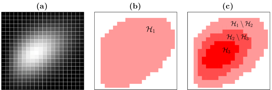
Figure 1: Model accounts implicitly for spatial structure. Panel a: The environment consists of a large number of sites. Each site is characterized by a local stress. Darker colors denote more stressful conditions; for the example shown here, the lowest stress is found in the center of the environment. Panel b: A species can only occupy sites in which the local stress is below the stress tolerance of the species. The sites in which species 1 can establish, that is, the habitat $\mathcal{H}_{1}$ of species 1, is shaded. Panel c: Less stress tolerant species have a smaller habitat. Moreover, the habitat of a more stress tolerant species contains the habitat of a less stress tolerant species. The sites in which different combinations of species 1, 2 and 3 can establish are shaded. In habitat $\mathcal{H}_{1}\setminus\mathcal{H}_{2}$ only species 1 can establish; in habitat $\mathcal{H}_{2}\setminus\mathcal{H}_{3}$ species 1 and 2 can establish, but not species 3; in habitat $\mathcal{H}_{3}$ all three species 1, 2 and 3 can establish. The sizes of these habitats are $h_{1}-h_{2}$, $h_{2}-h_{3}$ and $h_{3}$, respectively. Due to the model assumption that dispersal is uniform over the environment, the detailed spatial structure is irrelevant, that is, the model dynamics depend only on $h_{1}$, $h_{2}$ and $h_{3}$.

We construct the model equations for the dynamical variables $p_{1},p_{2},\ldots,p_{S}$. First, we compute the probability $Q_{i|k}$ that species $i$ recruits a site in habitat $\mathcal{H}_{k}\setminus\mathcal{H}_{k+1}$. A standard computation gives, see Appendix A,

$$Q_{i|k}=L\bigg{(}\sum_{j=1}^{k}f_{j}p_{j}\bigg{)}\,f_{i}p_{i},$$ (4)

with $L(x)=\frac{1-\mathrm{e}^{-x}}{x}$. The probability $Q_{0|k}$ that a site in $\mathcal{H}_{k}\setminus\mathcal{H}_{k+1}$ remains empty is

$$Q_{0|k}=\mathrm{e}^{-\sum_{i=1}^{k}f_{i}p_{i}}.$$ (5)

We interpret the probability $Q_{i|k}$ as the fraction of sites of habitat $\mathcal{H}_{k}\setminus\mathcal{H}_{k+1}$ recruited by species $i$. This approximation is justified by the assumption that the number of sites is large.

The size of habitat $\mathcal{H}_{k}\setminus\mathcal{H}_{k+1}$ is equal to $h_{k}-h_{k+1}$. Multiplying by (4), we get the size of the part of habitat $\mathcal{H}_{k}\setminus\mathcal{H}_{k+1}$ that is occupied by species $i$ in generation $t+1$. Summing this product over $k\geq i$, we get the fraction of the environment that is occupied by species $i$ in generation $t+1$. Hence, using the shorthand notation $p_{i}\equiv p_{i}(t)$ and $p_{i}^{+}\equiv p_{i}(t+1)$, we find

$$p_{i}^{+}=\sum_{k=i}^{S-1}(h_{k}-h_{k+1})\,Q_{i|k}+h_{S}\,Q_{i|S}.$$ (6)

Equation (6) for $i=1,2,\ldots,S$ defines the dynamical system for the species occupancies $p_{1},p_{2},\ldots,p_{S}$.

It is instructive to write down model (6) for $S=2$ species,

$$p_{1}^{+} =(h_{1}-h_{2})\Big{(}1-\mathrm{e}^{-f_{1}p_{1}}\Big{)}$$

$$\quad+h_{2}\frac{f_{1}p_{1}}{f_{1}p_{1}+f_{2}p_{2}}\Big{(}1-\mathrm{e}^{-\big{(}f_{1}p_{1}+f_{2}p_{2}\big{)}}\Big{)}$$ (7a)

$$p_{2}^{+} =h_{2}\frac{f_{2}p_{2}}{f_{1}p_{1}+f_{2}p_{2}}\Big{(}1-\mathrm{e}^{-\big{(}f_{1}p_{1}+f_{2}p_{2}\big{)}}\Big{)}.$$ (7b)

Recall that species 1 is more stress tolerant than species 2 (because $h_{1}>h_{2}$, see (2)). Hence, whereas species 2 can only recruit in habitat $\mathcal{H}_{2}$, species 1 can recruit in habitats $\mathcal{H}_{1}\setminus\mathcal{H}_{2}$ and $\mathcal{H}_{2}$, corresponding to the two terms in (7a). In habitat $\mathcal{H}_{1}\setminus\mathcal{H}_{2}$ species 1 is the only species to recruit sites; a fraction $\mathrm{e}^{-f_{1}p_{1}}$ of these sites remains empty. In habitat $\mathcal{H}_{2}$ both species 1 and 2 can recruit sites; a fraction $\mathrm{e}^{-(f_{1}p_{1}+f_{2}p_{2})}$ of these sites remains empty. The occupied sites are attributed to species 1 and 2 proportional to $f_{1}p_{1}$ and $f_{2}p_{2}$, respectively.

Limiting model for large fecundities

By simultaneously increasing the fecundities $f_{i}$, the number of empty sites diminishes. This suggests a limiting case of the general model (6) in which all sites are constantly occupied. To describe this limiting case, we introduce the fecundity scaling factor $\alpha$ and rescaled fecundities $\widehat{f}_{i}$. We consider the coupled limit

$$\alpha\to\infty\quad\text{and}\quad f_{i}\to\infty\quad\text{with}\ f_{i}=\alpha\widehat{f}_{i}\quad\text{for all $i$}.$$ (8)

In the limit (8) probability (4) of species $i$ recruiting an empty site in habitat $\mathcal{H}_{k}\setminus\mathcal{H}_{k+1}$ is

$$\widehat{Q}_{i|k}=\begin{cases}\displaystyle\frac{\widehat{f}_{i}p_{i}}{\textstyle\sum_{j=1}^{k}\widehat{f}_{j}p_{j}}&\text{if $p_{i}>0$}\\[12.0pt] 0&\text{if $p_{i}=0$.}\end{cases}$$ (9)

Hence, the site is occupied with certainty, except if all species that can recruit the site have become extinct. Species $i$ occupies the site with a probability proportional to $\widehat{f}_{i}p_{i}$. The corresponding dynamical system is

$$p_{i}^{+}=\sum_{k=i}^{S-1}(h_{k}-h_{k+1})\,\widehat{Q}_{i|k}+h_{S}\,\widehat{Q}_{i|S}.$$ (10)

The limiting model (10) is important because in the following sections we formulate some of the results for the general model (6) in terms of the limiting model (10).

3 Conditions for coexistence at equilibrium

Dynamical system (6) describes a community of $S$ species. Each species $i$ is characterized by two traits, its stress tolerance $h_{i}$ and its fecundity $f_{i}$. In this section we give the conditions on the species traits $h_{i}$ and $f_{i}$ for species coexistence at equilibrium. The (local) stability of the equilibria is studied in the next section.

We denote the set of all $S$ species by $\mathcal{S}=\{1,2,\ldots,S\}$. Each subset $\mathcal{C}\subset\mathcal{S}$ corresponds to a potential coexistence equilibrium.

Definition 1 (Coexistence equilibrium)

Consider a subset $\mathcal{C}\subset\mathcal{S}$. We call an equilibrium $(\widetilde{p}_{1},\widetilde{p}_{2},\ldots,\widetilde{p}_{S})$ of dynamical system (6) an equilibrium with coexistence set $\mathcal{C}$ if $\widetilde{p}_{i}>0$ for all $i\in\mathcal{C}$ and $\widetilde{p}_{i}=0$ for all $i\in\mathcal{S}\setminus\mathcal{C}$.

To formulate the coexistence conditions, it is convenient to introduce the inverse fecundities $g_{i}=\frac{1}{f_{i}}$. We exclude non-generic parameter combinations by the following assumption.

Assumption 1 (Genericity of parameters)

We assume that the species traits $h_{i}$ and $f_{i}$, $i=1,2,\ldots,S$, satisfy the following conditions:

• the parameters $h_{i}$, $i=1,2,\ldots,S$, are positive and arranged in decreasing order,

  $$h_{1}>h_{2}>\ldots>h_{S};$$ (11)

• the parameters $f_{i}$, $i=1,2,\ldots,S$, are positive and mutually different;

• the following ratios are mutually different and different from 1:

  $$\frac{h_{i}}{g_{i}},\ i=1,2,\ldots,S\qquad\text{and}\qquad\frac{h_{i}-h_{j}}{g_{i}-g_{j}},\ i,j=1,2,\ldots,S,\ i\neq j,$$

  with $g_{i}=\frac{1}{f_{i}}$.

The following result is proved in Appendix B.

Result 1 (Existence of equilibrium)

Suppose Assumption 1 is verified. Consider a subset $\mathcal{C}=\{i_{1},i_{2},\ldots,i_{C}\}\subset\mathcal{S}$ with $i_{1}<i_{2}<\ldots<i_{C}$. Then there exists an equilibrium with coexistence set $\mathcal{C}$ if and only if the following inequalities are satisfied:

$$1<\frac{h_{i_{1}}-h_{i_{2}}}{g_{i_{1}}-g_{i_{2}}}<\frac{h_{i_{2}}-h_{i_{3}}}{g_{i_{2}}-g_{i_{3}}}<\ldots<\frac{h_{i_{C-1}}-h_{i_{C}}}{g_{i_{C-1}}-g_{i_{C}}}<\frac{h_{i_{C}}}{g_{i_{C}}}.$$ (12)

If an equilibrium $(\widetilde{p}_{1},\widetilde{p}_{2},\ldots,\widetilde{p}_{S})$ with coexistence set $\mathcal{C}$ exists, then the equilibrium occupancies $\widetilde{p}_{i_{k}}>0$ are given by

$$\widetilde{p}_{i_{1}} =g_{i_{1}}\;\Lambda\bigg{(}\frac{h_{i_{1}}-h_{i_{2}}}{g_{i_{1}}-g_{i_{2}}}\bigg{)}$$ (13a)

$$\widetilde{p}_{i_{k}} =g_{i_{k}}\Bigg{(}\Lambda\bigg{(}\frac{h_{i_{k}}-h_{i_{k+1}}}{g_{i_{k}}-g_{i_{k+1}}}\bigg{)}-\Lambda\bigg{(}\frac{h_{i_{k-1}}-h_{i_{k}}}{g_{i_{k-1}}-g_{i_{k}}}\bigg{)}\Bigg{)}\qquad\text{$k=2,3,\ldots,C-1$}$$ (13b)

$$\widetilde{p}_{i_{C}} =g_{i_{C}}\Bigg{(}\Lambda\bigg{(}\frac{h_{i_{C}}}{g_{i_{C}}}\bigg{)}-\Lambda\bigg{(}\frac{h_{i_{C-1}}-h_{i_{C}}}{g_{i_{C-1}}-g_{i_{C}}}\bigg{)}\Bigg{)},$$ (13c)

where $\Lambda$ denotes the inverse function of $x\mapsto\frac{x}{1-\mathrm{e}^{-x}}$. Finally, if an equilibrium with coexistence set $\mathcal{C}$ exists, then there is no other equilibrium with coexistence set $\mathcal{C}$.

Note that the function $\Lambda$ in Result 1 can be expressed in terms of the upper branch $W_{0}$ of the Lambert $W$ function,

$$\Lambda(x)=x+W_{0}(-x\,\mathrm{e}^{-x}),$$

see Appendix B for a derivation.

From (11) and (12) it follows that

$$g_{i_{1}}>g_{i_{2}}>\ldots>g_{i_{C-1}}>g_{i_{C}},$$ (14)

or

$$f_{i_{1}}<f_{i_{2}}<\ldots<f_{i_{C-1}}<f_{i_{C}}.$$

Species can coexist only if less tolerant species are more fecund, which indicates a trade-off between stress tolerance and fecundity. However, condition (14) is necessary but not sufficient for species coexistence. The tolerance-competition trade-off imposes stonger conditions than (14).

The necessary and sufficient condition for species coexistence can be represented graphically, see Figure 2. We represent the traits $(g_{i},h_{i})$ of all species in the $(g,h)$ plane (Figure 2a). To verify whether an equilibrium exists with coexistence set $\mathcal{C}$, we draw a broken line through the points corresponding to the species in set $\mathcal{C}$ (Figure 2b–d). The broken line consists of the following line segments:

• a line segment between species $i_{k}$ and $i_{k+1}$, for $k=1,2,\ldots,C-1$;

• a line segment from species $i_{1}$ with slope one towards larger $g$;

• a line segment from species $i_{C}$ to the origin $(g=0,h=0)$.

It follows from inequalities (11) and (14) that if there is an equilibrium with coexistence set $\mathcal{C}$, then the broken line should define an increasing function of $g$. Condition (12) expresses that the slopes of the line segments should decrease for increasing $g$. This corresponds to requiring that the function defined by the broken line is concave. If this condition is fulfilled, then there exists an equilibrium with coexistence set $\mathcal{C}$.

Examples of the broken-line construction are shown in Figure 2b–d. In panel b we check the coexistence of $\mathcal{C}=\{2,3,4\}$. The broken line is not concave, so that no equilibrium exists with coexistence set $\mathcal{C}$. In panels c and d we check the coexistence of $\mathcal{C}=\{2,4,5\}$ and $\mathcal{C}=\{3,5\}$, respectively. In both cases the broken line is concave, so that an equilibrium exists with coexistence set $\mathcal{C}$ coexist. For a specific set $\mathcal{C}$ of coexisting species, the equilibrium, if it exists, is unique. However, there can be different sets $\mathcal{C}$ of coexisting species for which an equilibrium exists. We show in Section 4 that only one of these equilibria is stable.

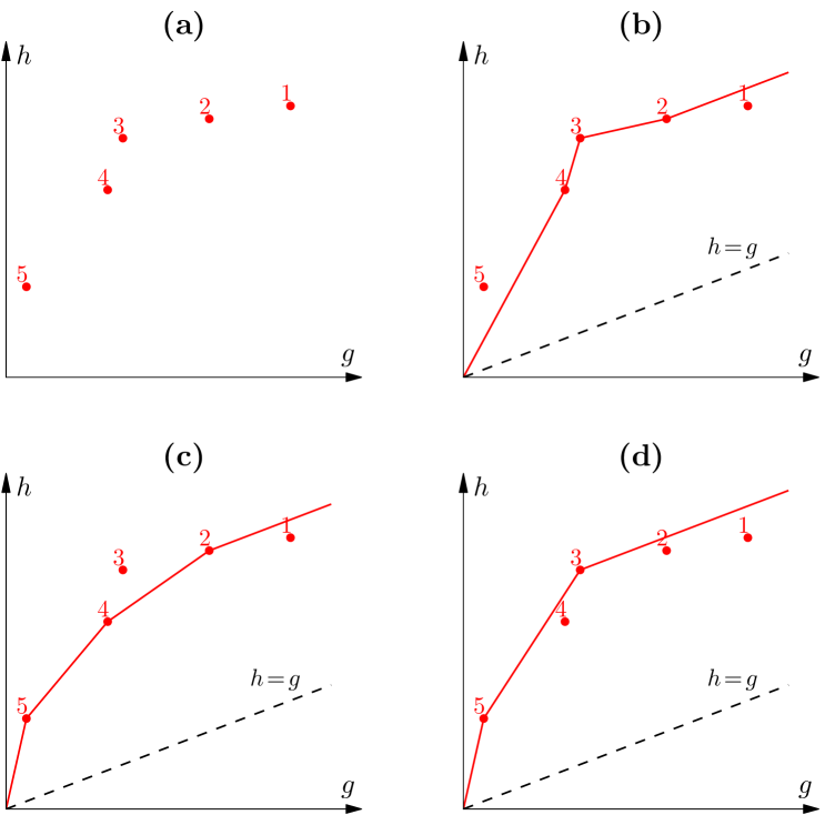
Figure 2: Graphical representation of the coexistence conditions (12) and the stability conditions (16). Panel a: The traits of $S=5$ species are represented in the $(g,h)$ plane; $g_{i}=\frac{1}{f_{i}}$ are inverse fecundities and $h_{i}$ are stress tolerances. Panel b: We check whether an equilibrium exists in which species 2, 3 and 4 coexist, and species 1 and 5 are absent (corresponding to $\mathcal{C}=\{2,3,4\}$). We draw a broken line through the species traits $(g_{i},h_{i})$ with $i\in\mathcal{C}$; the leftmost line segment passes through the origin; the rightmost line segment is parallel to the $h=g$ line (dashed line). Because the resulting function is not concave, there does not exist such an equilibrium. Panel c: We check whether an equilibrium exists in which species 2, 4 and 5 coexist, and species 1 and 3 are absent ($\mathcal{C}=\{2,4,5\}$). The same construction as in panel b gives a concave broken line. Hence, there exists such an equilibrium. Because the traits of species 3 lie to the left of and above the broken line, the equilibrium is unstable. Panel d: An equilibrium exists in which species 3 and 5 coexist, and species 1, 2 and 4 are absent ($\mathcal{C}=\{3,5\}$). Because the traits of all absent species lie to the right of and below the broken line, the equilibrium is stable.

A graphical construction for the equilibrium occupancies $\widetilde{p}_{i_{k}}$ is given in Figure 3. We start with the limiting model (10) for which Result 1 also holds. The limit (8) corresponds to replacing in (13) the function $\Lambda$ with the identity function. The resulting equilibrium occupancies $\widehat{p}_{i_{k}}$ are

$$\widehat{p}_{i_{1}} =g_{i_{1}}\;\frac{h_{i_{1}}-h_{i_{2}}}{g_{i_{1}}-g_{i_{2}}}$$ (15a)

$$\widehat{p}_{i_{k}} =g_{i_{k}}\bigg{(}\frac{h_{i_{k}}-h_{i_{k+1}}}{g_{i_{k}}-g_{i_{k+1}}}-\frac{h_{i_{k-1}}-h_{i_{k}}}{g_{i_{k-1}}-g_{i_{k}}}\bigg{)}\qquad\text{$k=2,3,\ldots,C-1$}$$ (15b)

$$\widehat{p}_{i_{C}} =g_{i_{C}}\bigg{(}\frac{h_{i_{C}}}{g_{i_{C}}}-\frac{h_{i_{C-1}}-h_{i_{C}}}{g_{i_{C-1}}-g_{i_{tC}}}\bigg{)}.$$ (15c)

The broken-line representation introduced in Figure 2 can be used to construct the occupancies $\widehat{p}_{i_{k}}$, see Figure 3a. The difference between (13) and (15) resides in the function $\Lambda$. We use the function $\Lambda$ to transform the slopes of the broken line of Figure 3a, see Figure 3b. We construct a new broken line with the transformed slopes, from which we obtain the occupancies $\widetilde{p}_{i_{k}}$, see Figure 3c.

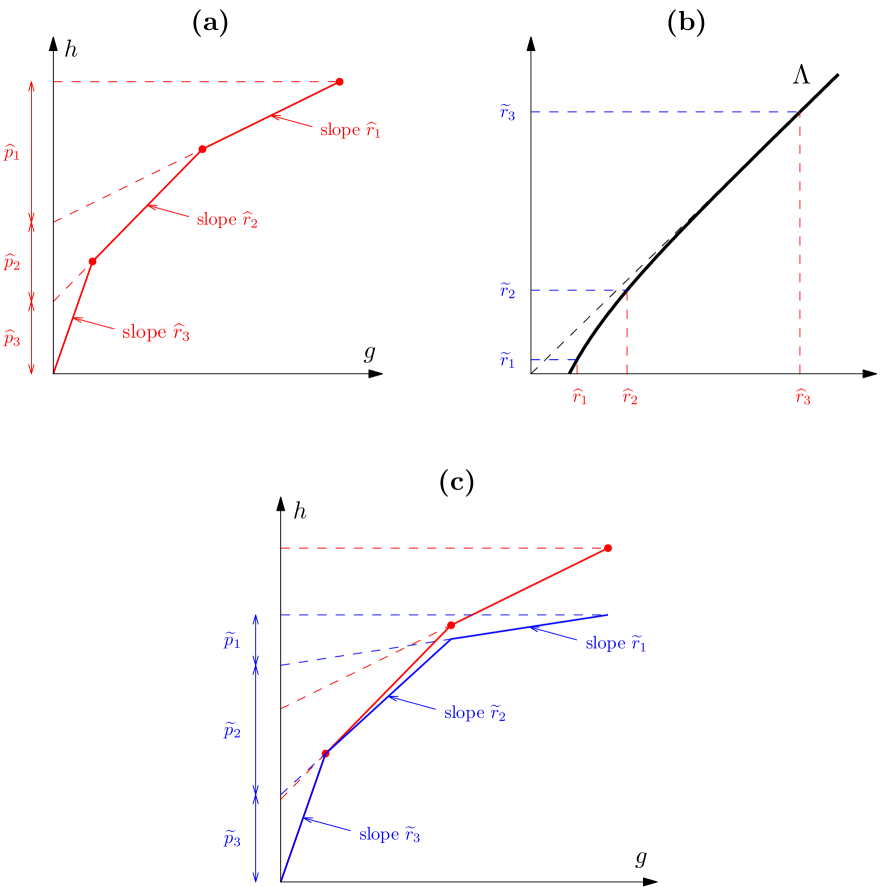
Figure 3: Graphical construction of the equilibrium occupancies. Panel a: We draw the traits of the species in the $(g,h)$ plane (red dots; there are $S=3$ species), and construct a broken line through the species traits, as shown in the figure (solid red line). By extending the line segment towards the $g=0$ axis (dashed red line), we obtain the equilibrium occupancies $\widehat{p}_{i}$. Panel b: For each of the $S$ slopes of the broken line in panel a, we compute a transformed slope using the function $\Lambda$. Panel c: We construct a broken line with the transformed slopes, as shown in the figure. Because the transformed slopes $\widetilde{r}_{i}=\Lambda(\widehat{r}_{i})$ are smaller than the initial slopes $\widehat{r}_{i}$, the new broken line (solid blue line) is a squeezed version of the initial broken line (solid red line). Using the same construction as in panel a, that is, by extending the line segments towards the $g=0$ axis (dashed blue line), we obtain the equilibrium occupancies $\widetilde{p}_{i}$.

Finally, we note that the last statement of Result 1 says that any two equilibria with the same coexistence set are the same equilibrium. Similar results have been reported for other dynamical systems, e.g., Boolean networks (vxx).

4 Stability of coexistence equilibrium

In Result 1 we have characterized the equilibria of dynamical system (6). There can be up to $2^{S}$ equilibria for a community of $S$ species. In this section we study the local stability of the equilibria. We show that there is only one locally exponentially stable equilibrium.

We state the stability conditions for an equilibrium of dynamical system (6). The result is proved in Appendix C.

Result 2 (Stability of equilibrium)

Suppose Assumption 1 is verified. Consider a subset $\mathcal{C}=\{i_{1},i_{2},\ldots,i_{C}\}\subset\mathcal{S}$ with $i_{1}<i_{2}<\ldots<i_{C}$. Consider an equilibrium $(\widetilde{p}_{1},\widetilde{p}_{2},\ldots,\widetilde{p}_{S})$ of dynamical system (6) with coexistence set $\mathcal{C}$. Then the equilibrium is locally exponentially stable if and only if the following inequalities are satisfied:

$$1>\frac{h_{j}-h_{i_{1}}}{g_{j}-g_{i_{1}}} j\in\mathcal{S}\setminus\mathcal{C} j<i_{1}$$ for all for which (16a)

$$\frac{h_{i_{k}}-h_{j}}{g_{i_{k}}-g_{j}}>\frac{h_{j}-h_{i_{k+1}}}{g_{j}-g_{i_{k+1}}} j\in\mathcal{S}\setminus\mathcal{C} k\in\{1,2,\ldots,C-1\}$$ for all and

for which $$i_{k}<j<i_{k+1}$$ (16b)

$$\frac{h_{i_{C}}-h_{j}}{g_{i_{C}}-g_{j}}>\frac{h_{j}}{g_{j}} \qquad\text{for all $j\in\mathcal{S}\setminus\mathcal{C}$ for which $i_{C}<j$}.$$ (16c)

We note that Result 2 implies that the equilibrium is locally asymptotically stable. Also note that the equilibrium cannot be asymptotically stable without being exponentially stable because Assumption 1 excludes the case in which some eigenvalues have modulus one.

Conditions (16) express that each of the $S-C$ species absent at equilibrium cannot invade the community of the $C$ coexisting species. Non-invasibility is a general necessary condition for stable species coexistence. Result 2 says that for dynamical system (6) non-invasibility is also a sufficient condition.

The stability conditions (16) can be formulated equivalently as

$$h_{j}-h_{i_{1}} <g_{j}-g_{i_{1}}$$ (17a)

$$h_{j}-h_{i_{k+1}} <\frac{h_{i_{k}}-h_{i_{k+1}}}{g_{i_{k}}-g_{i_{k+1}}}\,(g_{j}-g_{i_{k+1}})\qquad\text{for all $k\in\{1,2,\ldots,C-1\}$}$$ (17b)

$$h_{j} <\frac{h_{i_{C}}}{g_{i_{C}}}\,g_{j},$$ (17c)

for all $j\in\mathcal{S}\setminus\mathcal{C}$. Conditions (17) can be interpreted graphically, see Figure 2. We have explained how to determine whether a specific set $\mathcal{C}$ of $C$ species can coexist at equilibrium. The construction is based on a broken line containing the trait pairs $(g_{i},h_{i})$ of the $C$ coexisting species. Conditions (17) impose that the trait pairs $(g_{i},h_{i})$ of the other $S-C$ species absent at equilibrium should lie to the right of and below this broken line. For example, in panel c we check the stability of the coexistence equilibrium for $\mathcal{C}=\{2,4,5\}$. Species 3 lies to the left of and above the broken line, so the equilibrium is unstable. In panel d we check the stability of the coexistence equilibrium for $\mathcal{C}=\{3,5\}$. All species lie to the right of and below the broken line, so the equilibrium is locally stable.

In Figure 2 we have considered a community of $S=5$ species. It can be checked graphically that the broken line corresponding to $\mathcal{C}=\{3,5\}$ is the only broken line satisfying the conditions imposed by inequalities (12) and (16). That is, there is only one locally stable equilibrium. This suggests the following general result, proved in Appendix D:

Result 3 (Uniqueness of stable equilibrium)

Suppose Assumption 1 is verified. Then there is one and only one locally asymptotically stable equilibrium of dynamical system (6).

5 Continuous-time model

In this section we compare our model with the model proposed by ml10. Contrary to discrete-time dynamical system (6), the model of ml10 is formulated in continuous time. To allow comparison we construct the continuous-time equivalent of model (6), and argue that the model of ml10 can be recovered as a limiting model. We show that the equilibrium and stability results for model (6) also apply to the model of ml10.

The discrete-time model (6) assumes that the dynamics between two generations consist of two processes: first, all individuals die, vacating the occupied sites, and second, some of the sites are recruited by a new individual. In the continuous-time model, these two processes are no longer separated. Individuals die and vacate their site in a continuous manner, and simultaneously, sites are recruited by a new individual in a continuous manner.

We introduce the mortality rate $m$ and the recruitment rate $r$, both of which are assumed to be site- and species-independent. The recruitment process is modelled in the same way as in the discrete-time model. In an empty site of habitat $\mathcal{H}_{k}\setminus\mathcal{H}_{k+1}$, propagules of species $1,2,\ldots,k$ can regenerate. The probability that species $i$ recruits the site is given by $Q_{i|k}$ in (4). Note that there is a non-zero probability $Q_{0|k}$ that the site remains empty (until a following recruitment event). Hence, the effective recruitment rate for an empty site in $\mathcal{H}_{k}\setminus\mathcal{H}_{k+1}$ is $(1-Q_{0|k})r\leq r$.

We aim to construct the model equations for the dynamical variables $p_{1},p_{2},\ldots,p_{S}$. The rate of decrease of occupancy $p_{i}$ due to mortality is $m\,p_{i}$. The rate of increase of occupancy $p_{i}$ due to recruitment in habitat $\mathcal{H}_{k}\setminus\mathcal{H}_{k+1}$ is equal to $r\,Q_{i|k}$ times the size of the set of empty sites in $\mathcal{H}_{k}\setminus\mathcal{H}_{k+1}$. However, we cannot express the latter factor in terms of the species occupancies $p_{1},p_{2},\ldots,p_{S}$. We know that

$$\text{size of $\big{\{}$empty sites in habitat $\mathcal{H}_{1}$$\big{\}}$}=h_{1}-\sum_{i=1}^{S}p_{i},\\$$

but we do not know the distribution of the empty sites over the habitats $\mathcal{H}_{k}\setminus\mathcal{H}_{k+1}$. The variables $p_{1},p_{2},\ldots,p_{S}$ are not sufficiently informative to construct the model equations.

To solve the problem, we extend the set of dynamical variables. We introduce the set of occupancies $p_{ik}$ defined by

$$p_{ik}=\text{size of $\big{\{}$sites occupied by species $i$ in habitat $\mathcal{H}_{k}\setminus\mathcal{H}_{k+1}$$\big{\}}$}.$$

We have

$$\text{size of $\big{\{}$sites occupied by species $i$$\big{\}}$}=\sum_{k=i}^{S}p_{ik}=p_{i}$$

$$\text{size of $\big{\{}$occupied sites in habitat $\mathcal{H}_{k}\setminus\mathcal{H}_{k+1}$$\big{\}}$}=\sum_{i=1}^{k}p_{ik}$$

$$\text{size of $\big{\{}$empty sites in habitat $\mathcal{H}_{k}\setminus\mathcal{H}_{k+1}$$\big{\}}$}=h_{k}-h_{k+1}-\sum_{i=1}^{k}p_{ik}.$$

The rate of decreases of occupancy $p_{ik}$ due to mortality is $m\,p_{ik}$. The rate of increase of occupancy $p_{ik}$ due to recruitment is equal to $r\,Q_{i|k}$ times the size of the set of empty sites in habitat $\mathcal{H}_{k}\setminus\mathcal{H}_{k+1}$. Hence,

$$\frac{\mathrm{d}p_{ik}}{\mathrm{d}t}=-m\,p_{ik}+r\bigg{(}h_{k}-h_{k+1}-\sum_{j=1}^{k}p_{jk}\bigg{)}\,Q_{i|k}.$$ (18)

Recall that the probabilities $Q_{i|k}$ depend on the occupancies $p_{i}$, which can be expressed in terms of the occupancies $p_{ik}$. Hence, equation (18) for $i=1,2,\ldots,S$ and $k=i,i+1,\ldots,S$ defines an autonomous dynamical system.

It is interesting to note that the above-mentioned problem is not present in the limiting case of large recruitment rate $r$. If the recruitment rate $r$ is large, all sites are constantly occupied; as soon as an individual dies, a new individual recruits the vacated site. In that case, the effective rate of recruitment in $\mathcal{H}_{k}\setminus\mathcal{H}_{k+1}$ equals the rate of deaths in $\mathcal{H}_{k}\setminus\mathcal{H}_{k+1}$, given by $m(h_{k}-h_{k+1})$. The model equations are then