Experimental estimation of quantum discord for polarization qubit and the use of fidelity to assess quantum correlations

Abstract

We address the experimental determination of entropic quantum discord for systems made of a pair of polarization qubits. We compare results from full and partial tomography and found that the two determinations are statistically compatible, with partial tomography leading to a smaller value of discord for depolarized states. Despite the fact that our states are well described, in terms of fidelity, by families of depolarized or phase-damped states, their entropic discord may be largely different from that predicted for these classes of states, such that no reliable estimation procedure beyond tomography may be effectively implemented. Our results, together with the lack of an analytic formula for the entropic discord of a generic two-qubit state, demonstrate that the estimation of quantum discord is an intrinsically noisy procedure. Besides, we question the use of fidelity as a figure of merit to assess quantum correlations.

I Introduction

Quantum correlations are central resources for quantum technology. In the recent years, it has become clear that besides entanglement G novel concepts may be introduced to capture more specific aspects, such as quantum steering or quantum discord rev1 ; rev2 . Quantum discord has recently attracted considerable attention dis ; vogl ; rahimi ; galve ; lars ; bla12 ; haikka ; vas10 ; Yu2007 ; dakic ; gio10 ; fer12 ; chuan ; perinotti ; allegra ; bellomo ; mazzola ; chiuri ; daoud ; usha ; Xu10 ; add1 ; add2 ; add3 , as it captures and quantifies the fact that quantum information in a bipartite system cannot be accessed locally without causing a disturbance, at variance with classical probability distributions. Yet, the relevance of quantum discord as a resource is a highly debated topic Rod08 ; Bro13 , and a definitive answer may only come from experiments involving carefully prepared quantum states. This poses the problem of a precise characterization of quantum discord and of the design of optimized detection schemes bla12 ; ade13 .

For a given quantum state $\rho$ of a bipartite system $AB$, the total amount of correlations is defined by the quantum mutual information

$$I(\rho)=S(\rho_{A})+S(\rho_{B})-S(\rho),$$ (1)

where $S(\rho)=-\hbox{Tr}[\rho\log\rho]$ denotes von Neumann entropy and base two logarithm is employed. An alternative version of the quantum mutual information, that quantifies the classical correlations, is defined as

$$J_{A}=S(\rho_{B})-\min\sum_{k}p_{k}S(\rho_{B|k}).$$ (2)

where $\rho_{B|k}=\text{Tr}_{A}[\Pi_{k}\rho\Pi_{k}]/\text{Tr}[\Pi_{k}\rho\Pi_{k}]]$ is the conditional state of system $B$ after obtaining outcome $k$ on $A$, $\left\{\Pi_{k}\right\}$ are a projective measurements on $A$, and $p_{j}=\text{Tr}[\Pi_{k}\rho\Pi_{k}]]$ is the probability of obtaining the outcome $k$. While these two definitions are equivalent in classical information, the difference between them in quantum case defines entropic quantum discord

$$D_{A}(\rho)=\mathcal{I}(\rho)-\mathcal{J}_{A}(\rho).$$ (3)

An analogue quantity may be defined upon performing measurements on the system $B$. Notice also that different quantities, based on distances rather than entropy, have been proposed to measure quantum correlations dak10 ; pia12 , and recently measured experimentally without the need of tomographic reconstruction of the density matrix ade13 .

In this paper we address estimation of discord for different families of mixed states obtained from initially pure maximally entangled states. Our purpose is that of understanding what kind of measurements are really needed for a precise determination of this quantity. In particular, our setup is designed such to generate depolarized and/or phase-damped version of polarization Bell states $|\Phi^{+}\rangle$ and $|\Psi^{+}\rangle$. The first class of states is that of Werner (depolarized) states:

$$\rho_{W}(p)=p|\Psi\rangle\!\langle\Psi|+(1-p)\frac{\mathbb{I}}{2}\otimes\frac{\mathbb{I}}{2}$$ (4)

where $|\Psi\rangle=|\Phi^{+}\rangle,|\Psi^{+}\rangle$, $\mathbb{I}$ is the identity matrix, and $p$ is a mixing parameter related to the purity of $\rho_{W}$ by the formula $\mu=\hbox{Tr}\rho_{W}^{2}=(1+3p^{2})/4$. The second class of states we are going to investigate is given by phase-damped (decohered) version of Bell states, i.e.

$$\rho_{D}(p)=p|\Psi\rangle\!\langle\Psi|+(1-p)\sum_{kj}P_{kj}|\Psi\rangle\!\langle\Psi|P_{kj}\,,$$ (5)

where $|\Psi\rangle=|\Phi^{+}\rangle,|\Psi^{+}\rangle$, $P_{kj}=|k\rangle\langle k|\otimes|j\rangle\langle j|$ are the diagonal projectors over the standard basis, and the parameter $p$ is related to the purity by the relation $\mu=(1+p^{2})/2$.

Both the families (4) and (5) belong to the class of $X$-states (named after the shape of the nonzero portion of the density matrix). In addition, they may be written as

$$\rho=\frac{1}{4}\left(\mathbb{I}+\sum_{j=z,y,z}c_{j}\sigma_{j}\otimes\sigma_{j}\right)$$ (6)

where $\sigma_{j}$ are Pauli operators. Werner states (4) are obtained for $c_{1}=-c_{2}=c_{3}=p$, while decohered states (5) correspond to $c_{1}=-c_{2}=p$, $c_{3}=1$. For bipartite states of the form (6) a general analytic formula for the discord has been obtained Luo , leading to

$$D(\rho_{W})= \frac{1}{4}\left[3(1-p)\log(1-p)+(1+3p)\log(1+3p)\right]$$

$$-\frac{1}{2}\left[(1-p)\log(1-p)+(1+p)\log(1+p)\right]$$ (7)

$$D(\rho_{D})= \frac{1}{2}\left[(1-p)\log(1-p)+(1+p)\log(1+p)\right]$$ (8)

where we omit to denote the measured party since both families are made of symmetric states. For decohered states the optimal measurement to access the classical correlations is given by polarization measurement along the z-axis, whereas the fully symmetric structure of Werner states makes all the Pauli operators optimal.

Discord is a nonlinear functional of the density matrix and cannot, even in principle, correspond to an observable in strict sense. Its determination thus unavoidably involves an estimation procedure from a suitable set of feasible measurements LQE . In the following we present our experimental results about estimation of discord via tomographic reconstruction and investigate the possibility of its determination by a restricted set of measurements. We found that despite the fact that our states are well described, in terms of fidelity, by families of depolarized or phase-damped states, their discord may be largely different from that predicted for these classes of states, such that no reliable estimation procedure beyond tomography may be effectively implemented. Our results, together with the lack of an analytic formula for the discord of a generic two-qubit state gir11 , demonstrate that the estimation of quantum discord is an intrinsically noisy procedure.

In the next Section we describe our experimental setup as well as our tomographic reconstruction. The estimation of discord from experimental data is described in Section III whereas the discussion of results is reported in Section IV. Section V closes the paper with some concluding remarks.

II Experimental setup and reconstruction of the density matrix

In our setup polarization two-qubit states are generated using parametric down-conversion in a two-crystal geometry. In an optical crystal with type-I non-linearity, one photon of the pump beam decays into a pair of photons having same linear polarization. In our experiment (see Fig. 1) we have used Argon laser beam at 351 nm to pump two type-I beta barium borate (BBO) crystals fixed to have their optical axes in perpendicular planes.

A Glan-Thompson prism (GP) is used to project initial laser beam polarization to horizontal plane. Half-wave plate (WP₀) is then used to rotate at $45^{\circ}$ the polarization of the pump beam. First (second) BBO crystal has its optical axis in horizontal (vertical) plane and produce a pair of photons when pumped by a horizontally (vertically) polarized beam. Due to the coherent superposition of the two emissions the setup is suitable to create polarization entangled states of the form:

$$|\Psi_{\theta,\varphi}\rangle=\cos\theta|HH\rangle+e^{i\varphi}\sin\theta|VV\rangle$$ (9)

The quartz plates (QP) can be tilted to tune the phase between the two components. In the experiments reported in this paper we have fixed it to zero. We also set the superposition angle to $\theta=\pi/4$ in order to generate maximally entangled states. Non-linear crystals and quartz plates are placed in to a temperature-stabilized closed box for achieving stable phase-matching conditions all the time.

Figure 1: (Color online) Experimental setup to generate polarization photon pairs with variable quantum correlations and to perform tomographic reconstruction of the generated state.

The portion of our setup devoted to the characterization of the two-qubit states starts with a beam splitter (BS), which is used to split the initial (collinear) biphoton field into two spatial modes. In each output arm a quarter–wave (QWP_i) and a half–wave (WP_i) plates are placed, and followed by a linear polarizer and and interference filter (IF) with central wavelength at 702 nm (FWHM 10 nm). Avalanche photodiode detectors (D_i) are placed and the end and connected to a coincidence count scheme (CC).

In order to prepare basis states with both photons having vertical (horizontal) polarization we have rotated the half–wave plate WP₀ to feed only first (or second) crystal. To prepare basis states with orthogonal polarization of photons an additional half–wave plate(WP₃) may be introduced in the reflected arm. In the same way we are able to transform the initial $|\Phi^{+}\rangle=\frac{1}{\sqrt{2}}(|HH\rangle+|VV\rangle)$ to $|\Psi^{+}\rangle=\frac{1}{\sqrt{2}}(|HV\rangle+|VH\rangle)$ state. In addition, upon mixing maximally entangled and basis states obtained with different measurement times, we have analyzed Werner and phase-damped states with purity $\mu$ equal to $0.25$, $0.5$, $0.67$, $0.83$ and $1$.

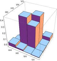
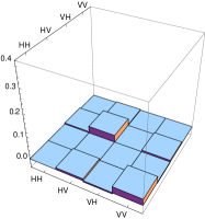
Figure 2: Real (left) and imaginary (right) part of the reconstructed density matrices of $|\psi^{+}\rangle$ (upper plot) and a $|\phi^{+}\rangle$ (lower plot) state

Two qubit quantum state tomography consists of set of projective measurements to different polarization states maxlik ; Kwiat ; cia09 ; OURs ; yu2011 . This is achieved using quarter–wave and half–wave plates in both channels. In particular, a set of independent two-qubit projectors $|\Psi_{\nu}\rangle\!\langle\Psi_{\nu}|$ with $\nu=0\dots 16$ were measured Kwiat . The probabilities $p_{\nu}=\langle\Psi_{\nu}|\rho|\Psi_{\nu}\rangle$ are estimated by the number of coincidence counts $n_{\nu}$ obtained measuring the projector $P_{\nu}$. In order to enforce positivity of the reconstructed state, we employ a Maximum Likelihood estimation scheme, where the density matrix is written as $\rho=T^{\dagger}T/\text{Tr}[T^{\dagger}T]$, $T$ being a complex lower triangular matrix. We have 16 real variables $t_{j}$ to be determined, with the physical density matrix given by $\rho_{L}(t_{1},t_{2},\dots,t_{16})$. The likelihood function assesses how the reconstructed density matrix $\rho_{L}(t_{1},t_{2},\dots,t_{16})$ reproduces the experimental data and it is a function of both the data counts $n_{\nu}$ (proportional to $p_{\nu}$) and the coefficients $t_{\nu}$, $\mathcal{L}(t_{1},t_{2},\dots,t_{16};n_{1},n_{2},\dots,n_{16})$. In the Gaussian approximation Kwiat the log-likelihood function for a given data count set $\{n_{\nu}\}_{\nu=1}^{16}$ is given by

$$\mathcal{L}(t_{1},t_{2},\dots,t_{16})=$$

$$N_{T}\sum_{\nu=1}^{16}\frac{(\langle\Psi_{\nu}|\rho_{L}(t_{1},t_{2},\dots,t_{16})|\Psi_{\nu}\rangle-n_{\nu})^{2}}{2\langle\Psi_{\nu}|\rho_{L}(t_{1},t_{2},\dots,t_{16})|\Psi_{\nu}\rangle}$$ (10)

where $N_{T}=\sum_{\nu=1}^{4}n_{\nu}$ is a constant proportional to the total number of runs. By numerically maximizing the log-likelihood over the coefficients $t_{1},t_{2},\dots,t_{16}$, we obtain the ML density matrix. In Fig. 2 we report the the reconstructed density matrices for the $|\psi^{+}\rangle$ (upper plot) and a $|\phi^{+}\rangle$ (lower plot) states. We also performed tomography for Werner and phase-damped states of the form (4) and (5) states with (theoretical) purity $\mu$ equal to $0.25$, $0.5$, $0.67$, $0.83$ and $1$. The resulting density matrices are very close to those expected theoretically. In fact, the fidelities of the experimentally reconstructed two-qubit states to Werner and phase-damped models are very high: all being larger than 0.96, and most of them larger than 0.98. The same is true for the values of the purity, as obtained from the reconstructed density matrices. Results are summarized in Tables 1 and 2. Uncertainties are evaluated assuming that counts $n_{\nu}$ are Poissonian distributed, with mean equal to the experimental recorded value. Then, we numerically sample counts from Poisson distributions and reconstruct the corresponding density matrices by maximum likelihood method. In this way, we generate a sample of physical density matrices and for each one we compute the fidelity and the purity. The standard deviation associated to these values represents the uncertainty of these quantities as estimated from tomographic reconstruction gum .

$\mu\left(\hbox{th}\right)$	$F\left(\rho_{W}^{\phi}\right)$	$F\left(\rho_{W}^{\psi}\right)$
1	0.98 $\pm$ 0.02	0.988 $\pm$ 0.004
$0.83$	0.96 $\pm$ 0.01	0.962 $\pm$ 0.006
0.66	0.96 $\pm$ 0.02	0.973 $\pm$ 0.02
0.50	0.99 $\pm$ 0.01	0.99 $\pm$ 0.02
0.25	0.991 $\pm$ 0.009	0.991 $\pm 0.009$
$\mu\left(\hbox{th}\right)$	$F\left(\rho_{D}^{\phi}\right)$	$F\left(\rho_{D}^{\psi}\right)$
1	0.98 $\pm$ 0.02	0.988 $\pm$ 0.004
0.83	0.998 $\pm$ 0.002	0.995 $\pm$ 0.002
0.66	0.997 $\pm$ 0.002	0.996 $\pm$ 0.002
0.50	0.997 $\pm$ 0.002	0.998 $\pm$ 0.002

Table 1: Fidelity between the reconstructed states and the corresponding theoretical X-states belonging to the families of Werner and phase-damped $|\Phi^{+}\rangle$ or $|\Psi^{+}\rangle$ states.

$\mu\left(\hbox{th}\right)$	$\mu_{T}\left(\rho_{W}^{\phi}\right)$	$\mu_{X}\left(\rho_{W}^{\phi}\right)$	$\mu_{T}\left(\rho_{W}^{\psi}\right)$	$\mu_{X}\left(\rho_{W}^{\psi}\right)$
1	0.96$\pm$0.04	0.996$\pm$0.002	0.984$\pm$0.08	0.995$\pm$0.002
0.83	0.79$\pm$0.04	0.84$\pm$0.01	0.82$\pm$0.03	0.87$\pm$0.01
0.66	0.66$\pm$0.04	0.68$\pm$0.02	0.66$\pm$0.03	0.69$\pm$0.02
0.50	0.48$\pm$0.03	0.46$\pm$0.01	0.47$\pm$0.02	0.52$\pm$0.01
0.25	0.259$\pm$0.006	0.25$\pm$0	0.267$\pm$0.007	0.25$\pm$0
$\mu\left(\hbox{th}\right)$	$\mu_{T}\left(\rho_{D}^{\phi}\right)$	$\mu_{X}\left(\rho_{D}^{\phi}\right)$	$\mu_{T}\left(\rho_{D}^{\psi}\right)$	$\mu_{X}\left(\rho_{D}^{\psi}\right)$
1	0.96$\pm$0.04	0.996$\pm$0.002	0.984$\pm$0.008	0.995$\pm$0.002
0.83	0.81$\pm$0.04	0.86$\pm$0.05	0.79$\pm$0.02	0.82$\pm$0.01
0.66	0.63$\pm$0.02	0.67$\pm$0.03	0.64$\pm$0.02	0.65$\pm$0.01
0.50	0.501$\pm$0.001	0.5$\pm$0	0.504$\pm$0.003	0.502$\pm$0.002

Table 2: Purity of the reconstructed states as estimated from tomography and from the X-state model.

III Estimation of discord

In order to estimate the value of discord, different techniques have been employed and compared. The first method is to employ two-qubit tomography of the state to estimate its density matrix and then determine the quantum discord from its definition in Eq. (3). This is done in two steps: At first we evaluate the quantum mutual information in Eq. (1), which requires the reconstructed density matrix only. Then the classical correlations are computed using Eq. (2). The minimization over all possible measurements is performed numerically, without assuming any specific form for the state. In fact, despite the high fidelity, the experimentally reconstructed density matrices do not have an exact X-shape, as shown in Fig. 2. This is due to fluctuations in the coincidence counts. In order to evaluate how this fluctuations propagate into fluctuations of the discord we have again assumed that counts $n_{\nu}$ are Poissonian distributed and generated a set of physical density matrices by Monte Carlo sampling of the coincidence counts. The standard deviation associated to these discord values is the uncertainty associated with the estimated value of discord via tomographic technique.

As an alternative method to evaluate discord, we may use partial tomography as follows. The evaluation of the quantum mutual information (1) is done as above. Then, we estimate the classical correlations (2) explicitly performing the optimal measurement and using partial tomography to determine the conditional states and in turn their entropy. To this aim, the quarter-wave and half-wave plates (QWP₁, WP₁) were used in one transmitted arm after the beam splitter to perform tomographic procedures only on the single photon state. No transformation was performed in reflected arm, that is, QWP₂ and WP₂ were removed from setup. As mentioned in the introductory Section, the optimal projection operator, minimizing the sum in Eq. (2), is $\sigma_{z}$ for both the families of mixed states Luo . Of course this technique is less general than the previous one since, strictly speaking, $\sigma_{z}$ is the optimal measurement only for states that are exactly Werner or phase-damped states. On the other hand, the large values of fidelity suggest that optimal measurement are not very far from the theoretical one, as well as the corresponding values of the classical correlations. We have validated this assumption a priori, by numerical evaluation of the optimal measurement (see the following paragraph and Fig. 3), and a posteriori, by comparing the resulting values of the discord with the results obtained from full tomography of the two qubit states.

The results about the optimization of measurement are summarized in Fig. 3 for some of the states of Table 1. We show the optimal measurement angle $\theta$ for the set of physical density matrices obtained by Monte Carlo sampling of the coincidence counts. The optimization has been performed over projective measurements of the form $\sigma(\theta,\phi)=\Pi_{0}-\Pi_{1}$, where $\Pi_{k}=\frac{1}{2}({\mathbb{I}}+\mathbf{n}_{k}.\mathbf{\sigma})$, $\mathbf{n}_{0}=(\sin\theta\cos\phi,\sin\theta\sin\phi,\cos\theta)$ and $\mathbf{n}_{0}\perp\mathbf{n}_{1}$. As it is apparent from the plot the optimal measurement is close to $\sigma_{z}$ (i.e. $\theta=0$) for the entire sample, and the fluctuations are small.

Figure 3: Optimal measurement to achieve classical correlations for some of the states generated in our experiments. We report the distribution of optimal angles $\theta$ for a set of 900 density matrices obtained by Monte Carlo sampling of coincidence counts. The left panel is for a phase-damped $|\Psi^{+}\rangle$ state with purity $\mu=0.66$ and the right panel for an unperturbed $|\Phi^{+}\rangle$ state.

The excellent agreement of the reconstructed states with the theoretical (Werner and phase-damped) models also suggests a third method to access discord: Upon assuming that our generated states belong to the families of single-parameter mixed states $\rho_{W}(p)$ and $\rho_{D}(p)$, we may estimate the value of discord using Eqs. (I) and (8), i.e. by estimating only the single parameter $p$. An estimator for this quantity may be determined using any function linking the mixing $p$ to the number of coincidence counts. Actually, we dispose of four of these functions for Werner states, and of two for decohered states. They are given by

$$\frac{1+(-1)^{\nu}p}{4}=\frac{n_{\nu}}{N_{T}}\quad\nu=1,2,3,4\quad\text{for }\rho_{W}(p)\hfill,$$ (11)

$$\frac{1-(-1)^{\frac{\nu}{2}}p}{4}=\frac{n_{\nu}}{N_{T}}\quad\nu=10,16\quad\text{for }\rho_{D}(p)\hfill.$$ (12)

We have used the above relations to build a randomized estimator for $p$ for both families and have evaluated their precision using Monte Carlo sampling of data (again assuming a Poissonian distribution for counts).

IV Results and discussion

In Table 3 we report the estimated values of quantum discord for depolarized and phase-damped $|\Phi^{+}\rangle$ and $|\Psi^{+}\rangle$ states, together with experimental uncertainties. We compare the values obtained via total and partial tomography with the determination achieved by assuming the single-parameter X-state model.

$\left[\rho_{W}^{\phi}\right]$	$\mu\left(\hbox{th}\right)$	TT	PT	$\rho_{W}^{\phi}(p)$
	1	0.9$\pm$0.1	0.9$\pm$0.1	0.997$\pm$0.002
	0.83	0.59$\pm$0.07	0.7$\pm$0.1	0.76$\pm$0.02
	0.66	0.47$\pm$0.05	0.6$\pm$0.1	0.56$\pm$0.02
	0.50	0.24$\pm$0.03	0.35$\pm$0.09	0.29$\pm$0.02
	0.25	0.009$\pm$0.007	0.04$\pm$0.04	0$\pm$9$\;10^{-7}$
$\left[\rho_{D}^{\phi}\right]$	$\mu\left(\hbox{th}\right)$	TT	PT	$\rho_{D}^{\phi}(p)$
	0.83	0.53$\pm$0.08	0.53$\pm$0.08	0.6$\pm$0.1
	0.66	0.20$\pm$0.04	0.20$\pm$0.04	0.26$\pm$0.05
	0.50	0.013$\pm$0.006	0.01$\pm$0.01	0$\pm$1$\;10^{-8}$
$\left[\rho_{W}^{\psi}\right]$	$\mu\left(\hbox{th}\right)$	TT	PT	$\rho_{W}^{\psi}(p)$
	1	0.94$\pm$0.03	0.94$\pm$0.03	0.989$\pm$0.005
	0.83	0.67$\pm$0.05	0.70$\pm$0.09	0.79$\pm$0.02
	0.66	0.47$\pm$0.04	0.5$\pm$0.1	0.57$\pm$0.02
	0.50	0.25$\pm$0.04	0.30$\pm$0.08	0.37$\pm$0.02
	0.25	0.009$\pm$0.007	0.04$\pm$0.02	0$\pm 1\;10^{-10}$
$\left[\rho_{D}^{\psi}\right]$	$\mu\left(\hbox{th}\right)$	TT	PT	$\rho_{D}^{\psi}(p)$
	0.83	0.49$\pm$0.04	0.48$\pm$0.04	0.53$\pm$0.03
	0.66	0.21$\pm$0.03	0.20$\pm$0.03	0.23$\pm$0.02
	0.50	0.008$\pm$0.005	0.016$\pm$0.001	0.003$\pm$0.003

Table 3: Estimation of discord the families of $\phi$- and $\psi$-states generated in our experiments. We report the determination obtained from total (TT) and partial (PT) tomography, and from the single-parameter X-state model.

In order to better compare these values, we also summarize them in Fig. 4. As it is apparent from the plots the two tomographic determinations are in good agreement within the uncertainties. More specifically, partial tomography (light gray squares) slightly overestimates the discord compared to total tomography (dark gray squares) for Werner states, while there is no appreciable difference for phase-damped states. On the other hand, despite the high-fidelity of the reconstructed states to the single-parameter (Werner or phase-damped) models, the discord estimated within this assumption (black square) is not always compatible with the corresponding tomographic determination. In particular, results from full tomography and the single-parameter models are never statistically compatible, and this happens also for partial tomography in some cases. This discrepancy questions the usefulness of fidelity in assessing quantum correlations. In fact, even if the reconstructed states have a very high fidelity to theoretical states $\rho_{W}(p)$ and $\rho_{D}(p)$, the estimated values of discord may be very different. The motivation behind this behavior is twofold. On the one hand, our states are not genuine X-states, despite the high value of fidelity. On the other hand, states that are very close in terms of fidelity may have very different values of discord. This argument, together with the fact that an analytic expression for the discord of arbitrary two qubits states cannot be obtained gir11 , leads to the conclusion that the only way to estimate the discord is through a tomography process, which itself is, in general, an intrinsically noisy procedure tn ; adv .

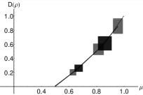
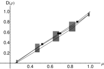
Figure 4: (Upper panels): Estimation of discord from total (dark gray) and partial (light gray) tomography and for the X-state model (black), with experimental errors as a function of the purity of the assumed Werner(left) and phase-damped (right) states obtained from state $|\Phi^{+}\rangle$. (Lower panels): the same for $|\Psi^{+}\rangle$

In order to illustrate explicitly the behavior of quantum discord for neighbouring states we have generated a set of random states (by Monte Carlo sampling starting from the recorded data set) in the vicinity of the reconstructed states, which are used as fixed reference states. We then compute both the fidelity $F(\varrho,\varrho_{0})$ between each random state and the reference one, as well as the discord of the generated state. Few examples of the resulting distributions are shown in Fig. 5. As it is apparent from the plot, states close, in terms of fidelity, to Werner states $\varrho_{W}^{\phi}$ or $\varrho_{W}^{\psi}$ with purity $\mu=0.66$, are also close in terms of discord, whereas there is a large fraction of states with a very high fidelity to $|\Psi^{+}\rangle$ or $|\Phi^{+}\rangle$ having a very different value of discord. In other words, discord is a highly non-linear function of the fidelity parameter, such that small deviations from its value may lead to very different values of discord.

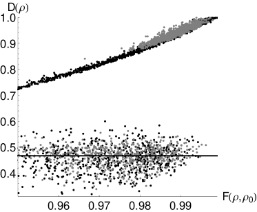
Figure 5: Distribution, in the $F$-$D$ (fidelity-discord) plane, of random states close, in terms of fidelity, to some states of Table 1. In the upper area of the plot we have gray points for states close to $|\Psi^{+}\rangle$ and black points for states close to $|\Phi^{+}\rangle$. In the lower area we have the same for states close to states $\varrho_{W}^{\psi}$ and $\varrho_{W}^{\phi}$ (purity $\mu=0.66$) respectively.

V Conclusions

In this paper we have addressed the experimental estimation of quantum discord for systems made of two correlated polarization qubits. We have compared the results obtained using full and partial tomographic methods and have shown that they are in good agreement within the experimental uncertainties. We have also computed the fidelity of the reconstructed states to suitable Werner and phase-damped states, and found very high values. This fact would in principle allows one to estimate quantum discord by assuming a single-parameter X-shape form for the reconstructed states, and extracting the mixing parameter from the data. Nonetheless, using the analytic expression for discord of Werner and decohered states, we found results that are statistically not compatible with the tomographic ones. This means that the assumed model is not usable, and that estimation of entropic discord for polarization qubits necessarily requires a tomographic reconstruction.

Indeed, states that are very close in terms of fidelity may have very different values of discord, i.e. discord is a quantity very sensitive to small perturbations. In fact, our states are not genuine X-states, despite the high value of fidelity, and this fact, together with the lack of an analytic expression for the quantum discord of a generic two-qubit state, leaves tomographic reconstruction as the sole reliable method to estimate quantum discord of polarization qubits. Our results also question the relevance and the role of fidelity as a tool in the evaluation of quantum correlations.

VI Acknowledgments

This work has been supported by MIUR (FIRB LiCHIS-RBFR10YQ3H) and by Compagnia di San Paolo.

References

- (1) M. Genovese, Phys. Rep. 413 (2005) 319.
- (2) K. Modi, A. Brodutch, H. Cable, T. Paterek, V. Vedral, Rev. Mod. Phys. 84, 1655 (2012).
- (3) L. C.Celeri J. Maziero, R. Serra, Int. J. Quantum Inf. 9, 1837 (2011).
- (4) A. Isar, Phys. Scripta, T 147, 014015 (2012).
- (5) U. Vogl, R. T. Glasser, Q. Glorieux, J. B. Clark, N. Corzo-Trejo, P. D. Lett, arXiv:1209.6079.
- (6) S. Rahimi-Keshari, C. M. Caves, T. C. Ralph, Phys. Rev. A 87, 012119 (2013).
- (7) F. Galve, F. Plastina, M. G. A. Paris, R. Zambrini, Phys. Rev. Lett. 110, 010501 (2013); F.Galve et al., EPL 96, 40005 (2011), Phys. Rev. A 83, 012102 (2011).
- (8) S. Lars A. Berni, M. Lassen, U. L. Andersen, Phys. Rev. Lett. 109, 030402 (2012);
- (9) R. Blandino, M. G. Genoni, J. Etesse, M. Barbieri, M. G. A. Paris, P. Grangier, R. Tualle-Brouri, Phys. Rev. Lett 109, 180402 (2012).
- (10) P.Haikka, T. H. Johnson, S. Maniscalco., arXiv:1203.6469.
- (11) R. Vasile, P. Giorda, S. Olivares, M. G. A. Paris, S. Maniscalco, Phys. Rev. A 82, 012313 (2010).
- (12) T. Yu and J. H. Eberly, Quantum Inf. Comput. 7, 459 (2007).
- (13) B. Dakic, Y. O. Lipp, X. Ma, M. Ringbauer, S. Kropatschek, S. Barz, T. Paterek, V. Vedral, A. Zeilinger, . Brukner, P. Walther, arXiv:1203.1629; B. Dakic, V. Vedral, and . Brukner, Phys. Rev. Lett. 105, 190502 (2010)
- (14) P. Giorda, M. G. A. Paris, Phys. Rev. Lett. 105, 020503 (2010).
- (15) A. Ferraro, M. G. A. Paris, Phys. Rev. Lett 108, 260403 (2012).
- (16) T. K. Chuan, J. Maillard, K. Modi, T. Paterek, M. Paternostro, M. Piani, Phys. Rev. Lett. 109, 070501 (2012).
- (17) P.Perinotti, Phys. Rev. Lett. 108, 120502 (2012).
- (18) M.Allegra, P. Giorda, A. Montorsi, Phys. Rev. B 84, 245133 (2011).
- (19) B.Bellomo, G. Compagno, R. Lo Franco, A. Ridolfo, S. Savasta, Int. J. Quantum Inf. 9, 1665 (2011).
- (20) L. Mazzola, J. Piilo, S. Maniscalco, Phys. Rev. Lett. 104, 200401 (2010); Int. J. Quantum Inf. 9, 981 (2011).
- (21) A.Chiuri, G. Vallone, M. Paternostro, and P. Mataloni, Phys. Rev. A 84, 020304(R) (2011).
- (22) M. Daoud, R. A. Laamara, Int. J. Quantum Inf. 10, 1250060 (2012).
- (23) A. R. Usha Devi, A. K. Rajagopal, Sudha, Int. J. Quantum Inf. 9, 1757 (2011).
- (24) J S. Xu, X. Y. Xu, C. F. Li, C. J. Zhang, X.B. Zou, G. C. Guo, Nat. Commun. 1, 7 (2010).
- (25) B. Bellomo, G. L. Giorgi, F. Galve, R. Lo Franco, G. Compagno, R. Zambrini, Phys. Rev. A 85, 032104 (2012).
- (26) B. Bellomo, R. Lo Franco, G. Compagno, Phys. Rev. A 86, 012312 (2012).
- (27) R. Lo Franco, B. Bellomo, E. Andersson, G. Compagno, Phys. Rev. A 85, 032318 (2012).
- (28) C. A. Rodriguez-Rosario, K. Modi, A. Kuah, A. Shaji, and E. C. G. Sudarshan, J. Phys. A 41, 205301 (2008).
- (29) A. Brodutch, A. Datta, K. Modi, A. Rivas, C. A. Rodriguez-Rosario, Phys. Rev. A 87, 042301 (2013).
- (30) I. A. Silva, D. Girolami, R. Auccaise, R. S. Sarthour, I. S. Oliveira, T. J. Bonagamba, E. R. de Azevedo, D. O. Soares-Pinto, and G. Adesso, Phys. Rev. Lett. 110, 140501 (2013).
- (31) B. Dakic, V. Vedral, C. Brukner, Phys. Rev. Lett. 105, 190502 (2010).
- (32) M. Piani, Phys. Rev. A 86, 034101 (2012).
- (33) S. Luo, Phys. Rev. A 77, 042303 (2008).
- (34) M. G. A. Paris, Int. J. Quant. Inf. 7, 125 (2009).
- (35) D.Girolami and G. Adesso, Phys. Rev. A,83, 052108 (2011).
- (36) K. Banaszek, G. M. D’Ariano, M. G. A. Paris, M. F. Sacchi, Phys. Rev. A 61 10304 (2000) Check This!
- (37) D. F. James, P. G. Kwiat, W. J. Munro, and A. G. White, Phys. Rev. A 64, 052312 (2001).
- (38) S. Cialdi, F. Castelli, M. G. A. Paris, J. Mod. Opt. 56, 215 (2009).
- (39) Yu. I. Bogdanov, G. Brida, M. Genovese, S. P. Kulik, E. V. Moreva, and A. P. Shurupov, Phys. Rev. Lett., 105, 010404 (2010).
- (40) Yu. I. Bogdanov, G. Brida, I. D. Bukeev, M. Genovese, K. S. Kravtsov, S. P. Kulik, E. V. Moreva, A. A. Soloviev and A. P. Shurupov, Phys. Rev. A, 84, 042108 (2011).
- (41) BIPM, IEC, IFCC, ILAC, ISO, IUPAC, IUPAP and OIML 2008 Evaluation of Measurement Data—Supplement 1 to the Guide to the Expression of Uncertainty in Measurement—Propagation of distributions using a Monte Carlo method Joint Committee for Guides in Metrology, JCGM 101 http://www.bipm.org/utils/common/documents/jcgm/JCGM_101_2008_E.pdf
- (42) G. M. D’Ariano, M. G. A. Paris, Phys. Lett. A 233 49 (1997); Phys. Rev. A 60 518 (1999).
- (43) G. M. D’Ariano, M. G. A Paris, and M. F. Sacchi, Adv. Im. Electr. Phys. 128, 205 (2003).