PetIGA: A Framework for High-Performance Isogeometric Analysis

Abstract

We present PetIGA, a code framework to approximate the solution of partial differential equations using isogeometric analysis. PetIGA can be used to assemble matrices and vectors which come from a Galerkin weak form, discretized with Non-Uniform Rational B-spline basis functions. We base our framework on PETSc, a high-performance library for the scalable solution of partial differential equations, which simplifies the development of large-scale scientific codes, provides a rich environment for prototyping, and separates parallelism from algorithm choice. We describe the implementation of PetIGA, and exemplify its use by solving a model nonlinear problem. To illustrate the robustness and flexibility of PetIGA, we solve some challenging nonlinear partial differential equations that include problems in both solid and fluid mechanics. We show strong scaling results on up to $4096$ cores, which confirm the suitability of PetIGA for large scale simulations.

1 Introduction

Isogeometric analysis, a finite element method originally proposed in 2005 [1, 2], was originally motivated by the desire to find a technique for solving partial differential equations which would simplify or remove the problem of converting geometric descriptions for discretizations in the engineering design process. Once a design is born inside a Computer Aided Design (CAD) program, converting the CAD representation to an analysis-suitable form usually is a bottleneck of the engineering analysis process. Isogeometric methods aim to use CAD representations directly by using the Non-Uniform Rational B-spline (NURBS) basis, circumventing the need to generate an intermediate geometrical description. The term isogeometric reflects that as the finite element space is refined, the geometrical representation can be preserved exactly. NURBS technologies have been used in CAD for decades due to their properties, particularly the smoothness and ability to represent conic sections. The key insight of isogeometric analysis is to use the geometrical map of the NURBS representation as a basis for the push forward used in analysis. This allows isogeometric modeling to advance where predecessors have found limitations [3, 4, 5, 6].

In addition to the geometrical benefits, the basis is also well-suited to solving higher-order partial differential equations, such as the ones related to phase-field problems [7, 8, 9] or large deformation shell formulations [10, 11, 12]. Classical finite element spaces use basis functions which are $C^{0}$ continuous across element boundaries, making them unsuitable for higher-order problems using a primal Galerkin formulation. The NURBS-based spaces may be constructed to possess arbitrary degrees of inter-element continuity for any spatial dimension. These higher-order continuous basis functions have been numerically [13, 14, 15, 16] and theoretically [17, 18] observed to possess superior approximability per degree of freedom when compared to their $C^{0}$ counterparts. However, when used to discretize a Galerkin weak form, the higher-order continuous basis functions have also been shown to result in linear systems which are more expensive to solve with multifrontal direct solvers [19, 20] and iterative solvers [21]. These results motivate the development of efficient, scalable software frameworks which can mitigate the increase of cost.

This paper describes a scalable implementation of tensor-product, NURBS-based isogeometric analysis. Despite the fact that writing every piece of code from scratch is still common practice in research groups, we believe that reusable software should become the norm in the scientific community. Otherwise, years of accumulated expertise in the field are disregarded [22, 23], which is inconsistent with the open and incremental nature of scientific discovery. However, the choice to depend on existent software should not be made lightly. Software libraries require maintenance and development to adapt to changing software and hardware requirements. This means that they require both personnel and funding to continue to exist. Furthermore, interfacing with other libraries can require development work on the library side. Without willing developers to support and assist third parties in using their libraries, the process can become cumbersome. We believe the benefits outweigh the risks, yet these are factors to consider when one plans to reuse the work of others.

PETSc [24, 25, 26], the Portable Extensible Toolkit for Scientific Computation, is a collection of algorithms and data structures for the solution of scientific problems, particularly those modeled by partial differential equations. PETSc is applicable to a wide range of problem sizes, including extreme large-scale simulations, where high-performance parallel computation is a must. PETSc uses the message-passing interface (MPI) model for communication, but provides high-level interfaces with collective semantics so that typical users rarely have to make message-passing calls directly.

PETSc provides a rich environment for modeling scientific problems as well as for rapid algorithm design and prototyping. The library enables easy customization and extension of both algorithms and implementations. This approach promotes code reuse and flexibility. PETSc is object-oriented in style, with components that may be changed via a command-line interface at runtime. These components include:

• Index sets to describe permutations, indexing, renumbering, and communication patterns;

• Matrices and vectors that provide basic linear algebra abstractions;

• Krylov subspace methods and preconditioners that include multigrid and sparse direct solvers;

• Nonlinear solvers and time stepping algorithms; and

• Distributed arrays for parallelizing structured grid-based problems.

PETSc is also designed to be highly modular, enabling the interoperability with specialized parallel libraries like Hypre [27], Trilinos/ML [28], MUMPS [29], and others through a unified interface. Other scientific packages geared towards solving partial differential equations use components from PETSc (for example deal.II [30], FEniCS [31], libMesh [32], and PETSc-FEM [33]).

In this paper we describe an approach to reuse PETSc algorithms and data structures to obtain a high-performance framework designed for isogeometric analysis. We implement parallel vector and matrix assembly using PETSc data structures and interface into PETSc’s wide range of solvers. In section 2, we detail the implementation as well as the features of the framework. In section 3, we tackle a model problem for nonlinear applications, and go through all the steps to solve it using our framework. Finally we showcase applications in section 4 and discuss performance results in section 5. We call our framework PetIGA. It is freely available [34] and under active development.

2 Implementation

2.1 B-spline basis functions

Let $\Xi=\{\xi_{0},\dots,\xi_{m}\}$ be a non-decreasing sequence of real numbers, i.e., $\xi_{i}\leq\xi_{i+1},i=0,\dots,m-1$. The $\xi_{i}$ are called knots and $\Xi$ is the knot vector. By using the Cox–de Boor recursion formula [35, 36], the $i$th B-spline basis function of $p$-degree, $i=0,\dots,m-p-1$, denoted $B_{i,p}(\xi)$, is defined as

$$B_{i,0}\left(\xi\right) =\begin{cases}1\ \ \text{if }\xi_{i}\leq\xi<\xi_{i+1},\\ 0\ \ \text{otherwise,}\end{cases}$$ (1)

$$B_{i,p}\left(\xi\right) =\frac{\xi-\xi_{i}}{\xi_{i+p}-\xi_{i}}B_{i,p-1}(\xi)+\frac{\xi_{i+p+1}-\xi}{\xi_{i+p+1}-\xi_{i+1}}B_{i+1,p-1}(\xi).$$ (2)

Writing $B_{i,p}$ instead of $B_{i,p}(\xi)$ for brevity, the first derivative of a basis function is given by

$$B^{\prime}_{i,p}(\xi)=\frac{p}{\xi_{i+p}-\xi_{i}}B_{i,p-1}+\frac{p}{\xi_{i+p+1}-\xi_{i+1}}B_{i+1,p-1}.$$ (3)

Repeated differentiation of the previous expression produces the general formula for the $k$th derivative $B^{(k)}_{i,p}(\xi)$ of $B_{i,p}(\xi)$

$$B^{(k)}_{i,p}(\xi)=p\left(\frac{B^{(k-1)}_{i,p-1}}{\xi_{i+p}-\xi_{i}}+\frac{B^{(k-1)}_{i+1,p-1}}{\xi_{i+p+1}-\xi_{i+1}}\right).$$ (4)

Even though this is the standard way of expressing the basis functions, we compute basis values and derivatives using the more computationally efficient algorithms detailed in [37].

2.2 Tensor product basis functions

By using a tensor product structure, a one-dimensional basis can be extended to multi-dimensions. Here we write a three-dimensional extension of the one-dimensional B-spline basis. Let

$$\Xi=\{\xi_{0},\dots,\xi_{n+p+1}\},\ \mathrm{H}=\{\eta_{0},\dots,\eta_{m+q+1}\},\ \mathrm{Z}=\{\zeta_{0},\dots,\zeta_{o+r+1}\}$$

be knots vectors which define three sets of one-dimensional B-spline basis functions

$$\{B_{i,p}(\xi),i=0,\dots,n\},\ \{B_{j,q}(\eta),j=0,\dots,m\},\ \{B_{k,r}(\zeta),k=0,\dots,o\}$$

of degree $p$, $q$, and $r$, respectively. The three-dimensional B-spline basis functions are defined as

$$M_{ijk}(\xi,\eta,\zeta)=B_{i,p}(\xi)B_{j,q}(\eta)B_{k,r}(\zeta).$$ (5)

For the sake of notational convenience and dimension independence, we denote multi-dimensional B-spline basis functions as $M_{A}(\boldsymbol{\xi})$ in the following. For the particular case of three dimensions, $\boldsymbol{\xi}$ denotes the parametric coordinate $(\xi,\eta,\zeta)$ and $A$ is the global basis index, i.e., $A=i+j(n+1)+k(n+1)(m+1)$.

2.3 NURBS basis functions and derivatives

Given the B-spline basis functions $M_{A}(\boldsymbol{\xi})$, we can define the corresponding NURBS [37] basis as

$$N_{A}(\boldsymbol{\xi})=\dfrac{w_{A}M_{A}(\boldsymbol{\xi})}{w(\boldsymbol{\xi})}$$ (6)

where $w_{A}$ are the projective weights and the weighting function appearing in the denominator is

$$w(\boldsymbol{\xi})=\sum_{B}w_{B}M_{B}({\boldsymbol{\xi}})$$ (7)

Omitting the explicit dependence on ${\boldsymbol{\xi}}$ for notational convenience, derivatives of $w$ with respect to the parametric coordinates are simply

$$w_{,\alpha} =\dfrac{\partial w}{\partial\xi_{\alpha}}=\sum_{B}w_{B}M_{B,\alpha}$$ (8)

$$w_{,\alpha\beta} =\dfrac{\partial^{2}w}{\partial\xi_{\alpha}\partial\xi_{\beta}}=\sum_{B}w_{B}M_{B,\alpha\beta}$$ (9)

$$w_{,\alpha\beta\gamma} =\dfrac{\partial^{3}w}{\partial\xi_{\alpha}\partial\xi_{\beta}\partial\xi_{\gamma}}=\sum_{B}w_{B}M_{B,\alpha\beta\gamma}$$ (10)

Using the chain rule, the first, second, and third derivatives with respect to $\xi_{\alpha}$ of the rational basis function $N_{A}$ defined in (6) can be expressed as

$$N_{A,\alpha} =\dfrac{w_{A}M_{A,\alpha}-N_{A}w_{,\alpha}}{w}$$ (11)

$$N_{A,\alpha\beta} =\dfrac{w_{A}M_{A,\alpha\beta}-N_{A}w_{,\alpha\beta}}{w}$$

$$-\dfrac{N_{A,\beta}w_{,\alpha}+N_{A,\alpha}w_{,\beta}}{w}$$ (12)

$$N_{A,\alpha\beta\gamma} =\dfrac{w_{A}M_{A,\alpha\beta\gamma}-N_{A}w_{,\alpha\beta\gamma}}{w}$$

$$-\dfrac{N_{A,\alpha}w_{,\beta\gamma}+N_{A,\beta}w_{,\alpha\gamma}+N_{A,\gamma}w_{,\alpha\beta}}{w}$$

$$-\dfrac{N_{A,\beta\gamma}w_{,\alpha}+N_{A,\alpha\gamma}w_{,\beta}+N_{A,\alpha\beta}w_{,\gamma}}{w}$$ (13)

In (6), we gave a definition of the rational basis function in terms of its parametric coordinates. However, when using the isoparametric concept [38], we need to express derivatives in terms of spatial coordinates, not their parametric counterparts. Higher-order derivatives of the geometrical mapping and basis functions are not standard in the literature and are required if one is to solve a higher-order partial differential equations on a mapped geometry. For the sake of completeness, the derivation of these derivatives can be found in appendix A.

2.4 Periodic boundary conditions

Due to the prevalent use of open knot vectors by the IGA community, applications which require the enforcement of periodic boundary conditions typically do so by building a system of constraints on the coefficients. For example, in [39], the authors detail constraint equations which enforce $C^{1}$ periodicity. However, we prefer to build periodicity into the function space due to its simplicity and generality. We do this by unclamping the knot vector as in the parlance of [37]. Let $\Xi=\{\xi_{0},\ldots,\xi_{m}\}$ be an open (or clamped) knot vector which encodes a set of $p$-degree B-spline basis functions $\{B_{i,p}(\xi),i=0,\dots,n\}$, where $m=n+p+1$. Unclamping the knot vector for a desired continuity $C^{k}$ at the boundary, $0\leq k\leq p-1$, amounts to redefining $k+1$ knot values at the left and right ends.

$$\xi_{k-i} =\xi_{p}-\xi_{n+1}+\xi_{n-i},\quad 0\leq i\leq k,$$ (14)

$$\xi_{m-k+i} =\xi_{n+1}-\xi_{p}+\xi_{p+i+1},\quad 0\leq i\leq k.$$ (15)

In figure 1 we present a $C^{2}$ cubic B-spline space with varying orders of continuity across the periodic boundary. Each of these knot vectors was obtained by unclamping the open knot vector $\Xi=\{0,0,0,0,0.2,0.4,0.6,0.8,1,1,1,1\}$ using equations (14) and (15). Each unique basis is labeled with its global number and colored distinctly such that basis functions which pass the periodic interface may be identified.

Equations (14) and (15) are sufficient when utilizing the basis in the parametric domain. In cases where the parametric domain is mapped, the original control points of the mapping which correspond to the open knot vector also need to be unclamped. In [37, p. 577], algorithm A12.1 performs this operation but is limited to $C^{p-1}$ unclamping. We present a generalization in algorithm 1 for $C^{k}$ unclamping where U is the array of knots and Pw is the array of control points in homogeneous coordinates. In figure 2, we present the effect of our algorithm when applied to a quarter circular arc.

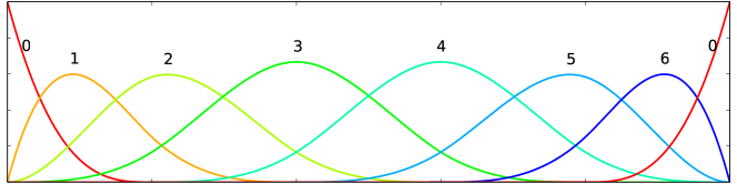
(a) $C^{0}$ periodicity, $\Xi=\{-0.2,0,0,0,0.2,0.4,0.6,0.8,1,1,1,1.2\}$

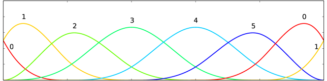
(b) $C^{1}$ periodicity, $\Xi=\{-0.4,-0.2,0,0,0.2,0.4,0.6,0.8,1,1,1.2,1.4\}$

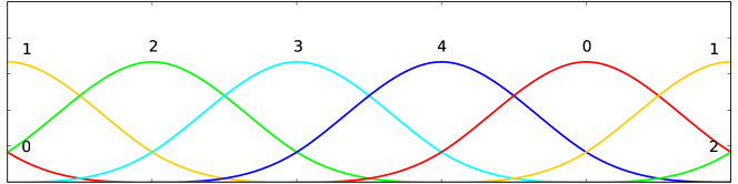
(c) $C^{2}$ periodicity, $\Xi=\{-0.6,-0.4,-0.2,0,0.2,0.4,0.6,0.8,1,1.2,1.4,1.6\}$

Figure 1: Three cases of periodicity for a $C^{2}$ cubic B-spline space. In each case, the open knot vector was unclamped using equations (14) and (15). Unique basis functions are labeled by their global numbering and colored distinctly.

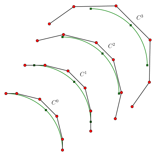
Figure 2: A quarter circular arc of degree four repeatedly unclamped by algorithm 1.

Algorithm 1 Pseudocode for unclamping curves.

UnclampCurve(n,p,k,U,Pw) {
  /* Input:
      n - index of last basis function
      p - polynomial degree
      k - continuity order
      U, Pw - knot vector and control points
    Output:
      U, Pw (modified in-place) */
  m = n + p + 1; /* index of last knot */
  for (i=0; i<=k; i++) /* Unclamp at left end */
    U[k-i] = U[p] - U[n+1] + U[n-i];
  for (i=p-k-1; i<=p-2; i++)
    for (j=i; j>=0; j--) {
      alpha = (U[p]-U[p+j-i-1])/(U[p+j+1]-U[p+j-i-1]);
      Pw[j] = (Pw[j]-alpha*Pw[j+1])/(1-alpha);
    }
  for (i=0; i<=k; i++) /* Unclamp at right end */
    U[m-k+i] = U[n+1] - U[p] + U[p+i+1];
  for (i=p-k-1; i<=p-2; i++)
    for (j=i; j>=0; j--) {
      alpha = (U[n+1]-U[n-j])/(U[n-j+i+2]-U[n-j]);
      Pw[n-j] = (Pw[n-j]-(1-alpha)*Pw[n-j-1])/alpha;
    }
}

After unclamping a knot vector, imposing periodic boundary conditions no longer requires the use of constraint equations. Periodicity can now be embedded into the function space by eliminating redundant basis functions in one of the domain boundaries. A practical way of dealing with this approach in a computer code is to properly map indices of basis functions that were eliminated to the corresponding ones that remain. In the non-periodic case, the number of basis functions is $n+1$. Imposing periodic boundary conditions with continuity order $k$ reduces the number of basis functions to $n-k$. Any basis function index $i$ outside the interval $\left[0,n-k-1\right]$ can be wrapped-around using the mapping  $i\mapsto\mathrm{mod}\left(i,n-k\right)$, where

$$\mathrm{mod}\left(a,b\right)=a-b\left\lfloor\frac{a}{b}\right\rfloor$$ (16)

and the symbol $\lfloor\cdot\rfloor$ denotes the floor function, i.e., $\lfloor x\rfloor$ is the largest integer not greater than $x$.

2.5 Adjacency graph

For numerical methods employing basis functions with local support, it is important to compute the adjacency graph of interacting degrees of freedom. This graph contains information required for the proper preallocation of sparse matrices implemented in compressed sparse row (CSR) or column (CSC) formats. This preallocation is crucial for efficient matrix assembly. Furthermore, prior knowledge of the sparse matrix nonzero pattern enables the use of specialized differentiation techniques, such as the approximation of Jacobian matrices by colored finite differences, see section 2.8.

Given an array of knots U encoding a set of B-spline basis functions of $p$-degree, algorithm 2 computes the left-most ($\ell$) and right-most ($r$) indices of the basis functions interacting with the $i$-th basis function. That is, the support of the basis function $N_{i,p}$ has non-empty intersection with the support of $N_{j,p}$, for $\ell\leq j\leq r$. In one dimension, all basis functions with indices in the set $\{\ell,\ell+1,\ldots,r-1,r\}$ are adjacent to the $i$-th basis function. For dimensions higher than one, the adjacency graph is computed from the index sets $\{\ell_{d},\ell_{d}+1,\ldots,r_{d}-1,r_{d}\}$ for each $d$-dimension using the tensor-product structure and numbering in lexicographical order. When imposing periodic boundary conditions with continuity order $k$, algorithm 2 may return indices outside the interval $\left[0,n-k-1\right]$. Again, the index mapping given in (16) has to be used to wrap-around index values.

Algorithm 2 Pseudocode for computing the adjacency graph.

BasisStencil(i,p,U,l,r) {
  /* Input:
      i - index of basis
      p - polynomial degree
      U - knot vector
     Output: l,r */
      l - index of left-most overlapping basis
      r - index of right-most overlapping basis */
  j = i;
  while (U[j] == U[j+1]) j++;
  l = j - p;
  j = i + p + 1;
  while (U[j] == U[j-1]) j--;
  r = j - 1;
}

Figure 3(a) presents a set of cubic basis functions which varies in inter-element continuity. Each basis is labeled by a global number and colored distinctly. Figure 3(b) shows the corresponding nonzero pattern for the sparse matrix obtained by applying algorithm 2 to each basis.

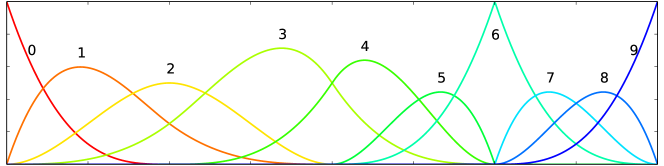
(a) A sample representative cubic B-spline basis consisting of four elements where the inter-element continuity progressively decreases according to the knot vector $\{0,0,0,0,2,4,4,6,6,6,8,8,8,8\}$.

(b) Nonzero structure where the function space represented above is used as test and trial functions in a Galerkin finite element method. Nonzero entries are indicated by a square.

Figure 3: Generation of the nonzero structure of matrices using algorithm 2.

2.6 Partitioning

In this section we describe the parallel partitioning and inter-process communication PetIGA uses. The ideas and techniques presented here closely resemble the ones used in PETSc to handle structured problems (through the DMDA component) as well as unstructured problems (through the DMPlex component), see [25]. However, PetIGA implements its own data structures tailored to the specifics of isogeometric analysis, particularly the use of higher-continuous, tensor-product polynomial spaces with possibly arbitrary continuity orders across discrete domains. In the following, element refers to a non-empty knot span (as defined in [2]) and node refers to an abstract entity that can encompass control points and weights of a NURBS geometry, control variables of either a scalar or vector field, unknown coefficients, and/or residual equation values.

Figure 4 depicts elements and nodes corresponding to a two-dimensional quadratic $C^{1}$ discrete space with $6\times 6$ elements and $8\times 8$ nodes. Both elements and nodes are labeled with an index which starts at zero and follows a natural numbering. In figure 4b, a subset of nodes is drawn inside a shaded region. These nodes correspond to basis functions with support on the element highlighted in figure 4a.

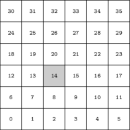
(a) Element grid.

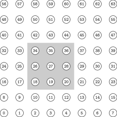
(b) Node grid.

Figure 4: A two-dimensional quadratic $C^{1}$ space with $6\times 6$ elements and $8\times 8$ nodes. The shaded region in figure 4b contains the nodes which correspond to basis functions with support on the element highlighted in figure 4a.

Given a $2\times 2$ grid of processes labeled from zero to three, figure 5 depicts a partition of the sets of elements and nodes. Figure 5a highlights a single element (drawn with a darker color) while figure 5b highlights its corresponding subset of nodes (drawn inside a shaded region). The highlighted element is assigned to process zero whereas the nodes inside the shaded region are assigned to different processes. Up to this stage, elements and nodes are still labeled according to the natural numbering defined in figure 4.

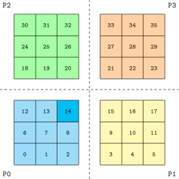
(a) Element partition.

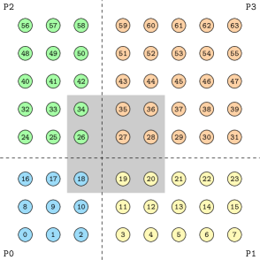
(b) Node partition and natural numbering.

Figure 5: The element and node grids in figure 4 are partitioned and distributed over a set of four processes $\{\texttt{P0,P1,P2,P3}\}$ arranged in a $2\times 2$ process grid. Elements and nodes are labeled according to the natural numbering, and assigned a distinct color that depends on which process they belong to. The shaded region in figure 5b contains the nodes related to the element highlighted in figure 5a.

Figure 6a defines a new node numbering. This global numbering is block-contiguous and follows the process numbering. The natural numbering in figure 5b and the global numbering in figure 6a define a bijective $\mathit{natural}~{}\mapsto~{}\mathit{global}$ mapping. The global numbering enhances locality, thus improving overall parallel performance. However, this numbering depends on the size and layout of the process grid. As the natural numbering does not depend on the partitioning, it is better suited for tasks involving data persistence, such as pre-/post-processing and checkpoint/restart. PetIGA employs the natural numbering when datafiles have to be read or written to disk, and uses the $\mathit{natural}~{}\mapsto~{}\mathit{global}$ mapping on the fly to convert to/from the global numbering.

The subset of nodes drawn inside the shaded region in figure 6a indicates that computations performed in the highlighted element in figure 5a would require communication with neighboring processes. As most distributed-memory parallel codes using the message-passing paradigm and dealing with grid-based methods, PetIGA efficiently handles inter-process communication by introducing augmented local grids at each process. Conceptually, a local grid is a sequential entity that belongs to a single process, while the global grid is a single entity that is distributed across processes. Within a local grid, two disjoint subsets of nodes can be distinguished: the strictly-local nodes which replicate the in-process subset of nodes of the global grid, and the ghost nodes which replicate global nodes assigned to neighboring processes. Figure 6b depicts the local grids of each process corresponding to the global grid in figure 6a. Nodes in the local grids are labeled with an index that starts at zero and defines the local numbering. Strictly-local nodes and ghost nodes are distinguished by assigning them a color that matches the process the corresponding global node is assigned to. For example, in figure 6b, in the local grid of process zero, blue nodes are strictly local nodes while the rest are ghost nodes. Data transfer between the global and local grids is managed through injective $\mathit{local}~{}\mapsto~{}\mathit{global}$ mappings defined within each process. Data associated to strictly-local nodes is handled with in-process memory transfers, while data associated to ghost nodes has to be communicated back and forth with neighboring processes. The communication costs increase with the number of ghost nodes, which in turn depend on the continuity order at inter-process interfaces: spaces of continuity $C^{k}$ lead to a number of ghost nodes proportional to $k+1$.

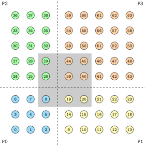
(a) Global node grid and global numbering.

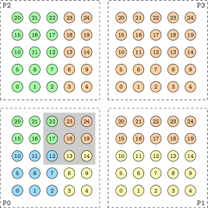
(b) Local node grids and local numberings.

Figure 6: Global and local node grids. Global nodes are colored according to the process they belong to, and labeled following a block-contiguous global numbering. Nodes in the local grids are labeled following a local numbering. The local grids in processes P0, P1, and P2 contain both strictly-local and ghost nodes, while the local grid in process P3 only contains strictly-local nodes. The shaded region in figure 6a is the same as in figure 5b. The nodes corresponding to the element highlighted in figure 5a are now fully contained within the local grid of process P0 as shown in figure 6b.

Lastly, figure 7 shows the layout of vectors and sparse matrices. The global vector in figure 7a is the concrete data structure used to store data associated with nodes from the global grid of figure 6a. Global vectors are distributed data structures built out of local one-dimensional arrays of floating point values. Similarly, the local vectors in figure 7b are the concrete counterparts of the local grids presented in figure 6b. These are nonetheless sequential data structures which are independent of each other. Global sparse matrices are distributed by rows across processes, as shown in figure 7c. Thanks to the locality induced by the block-contiguous global numbering, most of the entries within a process belong to the denser diagonal blocks. This in turn improves overall performance of global matrix-vector products.

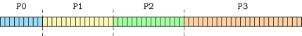
(a) Parallel layout of a global vector distributed across processes.

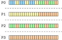
(b) Sequential layout of local vectors within each process.

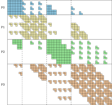
(c) Parallel layout of a global sparse matrix distributed by rows across processes.

Figure 7: Layout of vectors and sparse matrices.

2.7 Assembly

Through the pseudocode in algorithm 3, we describe how a residual vector coming from the discretization of a nonlinear partial differential equation is assembled in parallel. We use arrow symbols to reflect movement of memory, either within or across processes, and the equality symbol to signify when computation occurs. Given a global vector $\mathbf{U}$ which constitutes the current state of the solution to the nonlinear problem, we obtain the local vector $\mathbf{U}_{\ell}$ by gathering off-process values through inter-process communication and packing them together with process-owned values. The steps which follow are standard practice in finite element codes. We loop over all elements $e$ within a subpatch and gather solution and geometry coefficients $\mathbf{U}_{e}$ and $\mathbf{G}_{e}$, respectively. Then, we loop over quadrature points $q$ within the element and compute the set of nonzero basis functions and their spatial derivatives (which we collectively denote as $\left\{N_{q}\right\}$) as well as the determinant of the Jacobian the geometrical mapping $J_{q}$. The main difference between applications lies in the evaluation of the integrand at a quadrature point. This problem-specific evaluation routine has to be provided by the user. We then accumulate the quadrature point contributions $\mathbf{F}_{q}$ into the element residual vector $\mathbf{F}_{e}$, taking into account the quadrature weight $w_{q}$ and Jacobian determinant $J_{q}$. Each element residual $\mathbf{F}_{e}$ is then assembled into the global residual vector $\mathbf{F}$. In this step, PETSc automatically handles off-processor contributions by storing them in a cache which we designate as $\mathbf{F}_{\text{cache}}$. Finally, after the completion of the element loop, the cached contributions are communicated and assembled into the global vector $\mathbf{F}$. Matrices are assembled in a similar fashion. Again, the user only has to provide the problem-specific evaluation routine computing the integrand.

This approach to abstraction hides from the user the details of sparse matrix and vector assembly as well as parallelism. In turn, application codes are shorter and easier to read as they only contain code relevant to the physics of the modeled problem.

Algorithm 3 Pseudocode for global residual vector assembly.

1:function FormResidualVector($\mathbf{U}$)

2:     $\mathbf{U}_{\ell}\longleftarrow\mathbf{U}$

3:     for each element $e$ in subpatch do

4:         $\mathbf{U}_{e}\longleftarrow\mathbf{U}_{\ell}$

5:         $\mathbf{G}_{e}\longleftarrow\textsc{Geometry}(e)$

6:         for each quadrature point $q$ in element $e$ do

7:              $\mathbf{x}_{q},w_{q}\longleftarrow\textsc{Quadrature}(q)$

8:              $J_{q},\left\{N_{q}\right\}=\textsc{ShapeFuns}(\mathbf{x}_{q},\mathbf{G}_{e})$

9:              $\mathbf{F}_{q}=\textsc{Integrand}(\mathbf{x}_{q},\left\{N_{q}\right\},\mathbf{U}_{e})$

10:              $J_{q}w_{q}\mathbf{F}_{q}\overset{+\ }{\longrightarrow}\mathbf{F}_{e}$

11:         end for

12:         $\mathbf{F}_{e}\overset{+\ }{\longrightarrow}\mathbf{F}_{\text{cache}}$

13:     end for

14:     $\mathbf{F}_{\text{cache}}\overset{+\ }{\longrightarrow}\mathbf{F}$

15:     return $\mathbf{F}$

16:end function

2.8 Numerical differentiation

In the process of setting up new codes to solve nonlinear problems, one of the most time-consuming tasks involves the analytical derivation and subsequent coding of Jacobians. While exploring new ideas, models, and/or formulations to a problem, the expression of the nonlinear residual may change considerably, triggering the need to update the definition of the Jacobian. Moreover, the residual may contain complicated expressions (e.g., non-trivial material constitutive relations) whose derivatives are hard to obtain. Numerical differentiation can alleviate these burdens by providing a reliable way to approximate the Jacobian at the expense of additional computational time.

PETSc has built-in facilities within its nonlinear solver implementations to approximate Jacobians through numerical differentiation using two different techniques.

• Matrix-free Newton–Krylov. In this approach, a sparse matrix is never assembled. Instead, matrix-vector products involving the Jacobian are approximated within the Krylov linear solver using a first-order difference formula [40]. Even though this method can considerably reduce the memory requirements as well as the computational time, the lack of an actual matrix prevents using black-box preconditioning techniques. Unless the user can provide a (matrix-free) problem-specific preconditioner, this methodology is only suitable for nonlinear problems where the Jacobian is well conditioned. Otherwise, linear solvers may fail to converge or require large iteration counts and thus, residual evaluations, leading to a drastic increase in computational time. Matrix-free techniques can be enabled at runtime through the command line option -snes_mf.

• Colored finite differences. Unlike the previous approach, in this case a sparse matrix is assembled. A first-order difference formula is also used to form columns of the Jacobian matrix. Instead of computing columns individually, the method exploits sparsity by finding a partition of the set of columns using graph coloring techniques. In this way, many columns (more specifically, those having the same color) can be computed at once with a single global residual evaluation. We refer the reader to [41] for a thorough review on the topic. This black-box technique is sensible to use as long as the number of colors is small, which is the case in many discretization methods, and particularly linear finite elements. For higher-order finite element methods such as isogeometric analysis, the number of colors increases with the support of the basis functions. Colored finite differences techniques can be enabled at runtime through the command line option -snes_fd_color.

Being based on global residual evaluations, the approach PETSc takes is black-box and applicable to many discretization methods as it does not require explicit grid information. However, in the context of finite element methods, it is possible to exploit locality to develop an equivalent but more efficient implementation. Rather than computing the global Jacobian by evaluating the global residual vector, evaluations can instead be performed locally at the quadrature point level.

In the following, we recall the notation in section 2.7 and details of algorithm 3. In the local numerical differentiation approach available in our framework, the $k$-th column of the Jacobian matrix ${\partial\mathbf{F}_{q}}/{\partial\mathbf{U}_{e}}$ is computed at the quadrature point $q$ within an element $e$ using the following first-order finite difference approximation

$$\dfrac{\partial\mathbf{F}_{q}}{\partial\mathbf{U}_{e}}\mathbf{\hat{e}}_{k}\approx\dfrac{1}{\delta}\Big{(}\mathbf{F}_{q}(\mathbf{U}_{e}+\delta\mathbf{\hat{e}}_{k})-\mathbf{F}_{q}(\mathbf{U}_{e})\Big{)}$$ (17)

where $\mathbf{\hat{e}}_{k}$ denotes a vector with a $1$ in the $k$-th entry and zeros elsewhere, while $\delta$ is the difference step. Following the standard approach taken in [42], the difference step is computed as

$$\delta=\eta\sqrt{1+\|\mathbf{U}_{e}\|}$$ (18)

where $\eta$ should be set to the square root of the relative error in the evaluations of $\mathbf{F}_{q}$. As a default, this relative error is set to $\eta=\sqrt{\epsilon}$, where $\epsilon$ is the floating point machine epsilon (for double precision floating point numbers, $\epsilon\approx 2.22\times 10^{-16}$).

In appendix C, we present benchmark results comparing the numerical differentiation techniques mentioned in this section when applied to the three-dimensional Bratu equation. Even though explicitly coding the Jacobian is always the fastest way of computing this matrix, the local approach discussed in the previous paragraph seems to be a wiser choice when approximating it numerically.

We consider numerical differentiation to be an extremely useful feature to have at hand while prototyping and debugging. Ultimately, users should weigh computational overhead against development effort to decide whether numerical differentiation helps them achieve their particular goals.

2.9 Additional features

Our framework uses standard tensor product Gauss–Legendre quadrature. Tensor product Gauss–Lobatto quadrature rules are also available. Research on quadrature rules tailored to isogeometric analysis started in [43]. Support for optimal, B-spline-specific, quadrature rules is ongoing [44, 45, 46]. PetIGA also supports tensor product basis functions defined as Lagrange interpolants on either Newton–Cotes points (as in traditional finite elements) or Gauss–Lobatto points (as in spectral finite elements [47]). Although these methods are not the primary focus of our library, their availability can be useful to researchers willing to explore isogeometric analysis as an alternative to these well-established technologies. Even though PetIGA is geared towards handling Galerkin-type finite element formulations, the framework also supports isogeometric collocation methods [48].

Creation of initial geometries is a nontrivial task. Representation of a volume using NURBS is cumbersome and mostly developed manually, and bridging Computer Aided Design and Computer Aided Engineering is ongoing. To ease the handling of NURBS geometries we developed igakit [49], a Python package providing low-level interfaces to Fortran 90 routines in charge of manipulating knot vectors and control point data, as well as a high-level interface to simplify the definition of these geometries by hand. Details on using igakit to create geometries such as the one presented in figure 8 can be found in [50].

⬇

1from igakit.cad import *

2

3C0 = circle(radius=1)

4C1 = circle(radius=2)

5annulus = ruled(C0, C1)

6

7pipe = extrude(annulus,

8 displ=3,

9 axis=2,

10 ).reverse(2)

11

12elbow = revolve(annulus,

13 point=(3,0,0),

14 axis=(0,-1,0),

15 angle=Pi/2)

16

17bentpipe = join(pipe, elbow,

18 axis=2)

(a)

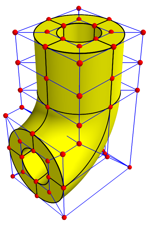
(b)

Figure 8: Generating a bent pipe (see [2], section 2.4) with igakit. The definition of this NURBS volume geometry entails four successive steps. First, an annulus is generated as a ruled surface between two concentric circles of different radii. Then, a pipe is generated by extruding the annulus along the appropriate direction. Next, an elbow is generated by revolving the base annulus $90^{\circ}$ around the appropriate axis. Finally, the pipe and the elbow are joined along one of the parametric directions.

3 Example

In this section we solve the Bratu equation as a model application to highlight some of the useful features users have access to when using our framework.

3.1 The Bratu equation

The Bratu equation is a nonlinear second-order boundary value problem [51]. The strong form of the equation can be stated as: find $u:\bar{\Omega}\rightarrow\mathbb{R}$ such that

$$-\Delta u =\lambda\exp(u),\quad \boldsymbol{x}\ \in\ \Omega,$$ (19)

$$u =0, \boldsymbol{x} \in \partial\Omega,$$ (20)

where $\bar{\Omega}$ is the unit square in $[0,1]^{2}$, $\partial\Omega$ denotes the domain boundary, $\Delta$ represents the Laplace operator, $u\equiv u(\boldsymbol{x})$ is a scalar field defined in $\Omega$ and $\lambda$ is a positive constant. No solution exists when $\lambda$ goes above $\lambda_{max}=6.80812$ as the equation possesses a bifurcation point. This equation models the steady-state of a nonlinear reaction and heat conduction problem, and results from a simplification of the solid-fuel ignition model.

Within the framework of Galerkin finite elements, let $\mathcal{V}$ denote the trial and weighting function spaces, where $\mathcal{V}$ belongs to $\mathcal{H}^{1}_{0}$, i.e., the Sobolev space of square-integrable functions with square-integrable first derivatives and zero value on $\partial\Omega$. The weak form is obtained by multiplying equation (19) by a test function $w$ and integrating by parts. The variational problem can then be defined as that of finding $u\in\mathcal{V}$ such that for all $w\in\mathcal{V}$

$$\left(\nabla w,\nabla u\right)_{\Omega}-\left(w,\lambda\exp\left(u\right)\right)_{\Omega}=0,$$ (21)

where $\left(\cdot,\cdot\right)_{\Omega}$ denotes the $\mathcal{L}^{2}$ inner product on domain $\Omega$. The finite-dimensional problem can then be formulated as: find $u^{h}\in\mathcal{V}^{h}$, where $\mathcal{V}^{h}\subset\mathcal{V}$, such that for all $w^{h}\in\mathcal{V}^{h}$

$$\left(\nabla w^{h},\nabla u^{h}\right)_{\Omega}-\left(w^{h},\lambda\exp\left(u^{h}\right)\right)_{\Omega}=0,$$ (22)

where $w^{h}$, $u^{h}$ and their respective gradients are defined as the linear combinations

$$w^{h} =\sum_{A}W_{A}N_{A}(\boldsymbol{x}), u^{h} =\sum_{A}U_{A}N_{A}(\boldsymbol{x}),$$ (23)

$$\nabla w^{h} =\sum_{A}W_{A}\nabla N_{A}(\boldsymbol{x}), \nabla u^{h} =\sum_{A}U_{A}\nabla N_{A}(\boldsymbol{x}),$$ (24)

where $N_{A}$ are the basis functions and $W_{A}$, $U_{A}$ are the control variables. Denoting $\mathbf{U}=\left\{U_{A}\right\}$ the vector of coefficients, we define the residual vector as $\mathbf{R\left(U\right)}=\left\{R_{A}\right\}$, where $R_{A}$ is obtained from (22)–(24) as

$$R_{A}=\left(\nabla N_{A},\nabla u^{h}\right)_{\Omega}-\left(N_{A},\lambda\exp\left(u^{h}\right)\right)_{\Omega},$$ (25)

As the problem is nonlinear, solving it with Newton’s method requires the specification of the Jacobian $\mathbf{J}=\partial\mathbf{R}/\partial\mathbf{U}$. In this particular problem, its entries are defined as

$$J_{AB}=\left(\nabla N_{A},\nabla N_{B}\right)_{\Omega}-\left(N_{A},\lambda\exp\left(u^{h}\right)N_{B}\right)_{\Omega}.$$ (26)

3.2 Implementation

To code a program within the framework, the user first needs to include the PetIGA C header file

⬇

1#include <petiga.h>

For the sake of simplicity, two macros are defined to set the dimensionality of the problem to two and implement the dot product of two-vectors

⬇

3#include <petiga.h>

To change the dimensionality of the problem to one or three, these two lines should be modified accordingly. Then, a C structure is used to handle the problem-specific parameter $\lambda$. This approach is preferred to the alternative of using global variables.

⬇

6#include <petiga.h>

7

8#define dim 2

The residual routine implementing equation (25) reads

⬇

10#include <petiga.h>

11

12#define dim 2

13#define dot(a,b) (a[0]*b[0]+a[1]*b[1])

14

15typedef struct {

16 double lambda;

17} Params;

18

19int Residual(IGAPoint p,const double U[],double R[],void *ctx) {

20 int a,nen = p->nen;

Recalling section 2.7, the residual routine constitutes the integrand to be evaluated at each quadrature point (line 9 of algorithm 3) to compute local contributions to the global residual vector. The Residual routine has the following arguments

• an input pointer p, of type IGAPoint, used as a quadrature point context holding discretization data required to perform the residual evaluation,

• an input floating point array U, which contains the local control variables gathered from the global vector $\mathbf{U}$, i.e., the coefficients corresponding to basis functions whose support contains the quadrature point, recall equations (23) and (24),

• an output floating point array R, where the routine is expected to return local contributions to be assembled in the global residual vector $\mathbf{R}$, recall equation (25),

• an input opaque pointer ctx, used to pass problem-specific information to the residual routine.

The code proceeds to declare the following local variables

• two integers a and nen, the first to be used as a loop index, while the second is initialized to the number of local basis functions,

• two pointers N0 and N1, initialized from data within the IGAPoint, used in the following for convenient access to the values of local basis functions ($0$th derivatives) and their first derivatives,

• two floating point variables u and grad_u to store the values of $u^{h}$ and $\nabla u^{h}$ at the quadrature point

• a floating point variable lambda to store the value of $\lambda$, initialized from the Params structure through the opaque pointer ctx.

Next, the routines IGAPointFormValue and IGAPointFormGrad are invoked to compute the values of $u^{h}$ and $\nabla u^{h}$ at the quadrature point, following equations (23) and (24). Finally, local residual contributions are computed in a loop following equation (25) by using the previously defined dot macro as well as the exp routine from the standard library of the C programming language. The quadrature weights and Jacobian determinant of the geometry mapping are handled internally, which slightly simplifies the coding.

The Jacobian routine implementing equation (26) reads

⬇

22#include <petiga.h>

23

24#define dim 2

25#define dot(a,b) (a[0]*b[0]+a[1]*b[1])

26

27typedef struct {

28 double lambda;

29} Params;

30

31int Residual(IGAPoint p,const double U[],double R[],void *ctx) {

32 int a,nen = p->nen;

The Jacobian routine is almost the same as the previous Residual routine. The main differences are the output floating point array J where the routine is expected to return local contributions to be assembled in the global Jacobian matrix $\mathbf{J}$, and the double-loop computing these contributions following equation (26).

The code of the main program routine then begins

⬇

34#include <petiga.h>

The first statement invokes the PetscInitialize routine, which internally handles the initialization of the PETSc library. This routine is fed with the command line arguments to the program. PETSc uses these arguments to build a database of options. These options are queried later.

The code proceeds to create and initialize an iga object of type IGA. The IGA type is a key component in PetIGA. This core data structure contains all the information related to discretization and parallel communication.

⬇

37#include <petiga.h>

38

39#define dim 2

40#define dot(a,b) (a[0]*b[0]+a[1]*b[1])

41

42typedef struct {

To properly setup the iga object, the user only needs to hardwire in code a couple of problem-specific parameters, and ask the framework to handle the rest at runtime through the options database

• the routine IGASetDim specifies the number of space dimensions, in this particular example it is set to two,

• the routine IGASetDof specifies the number of components in the solution, in this particular example it is set to one as the code is dealing with a scalar problem,

• the routine IGASetFromOptions queries the options database to let users change different properties of the discretization such as number of elements, polynomial degree and regularity of the approximation space, type of basis functions to use, quadrature rules, number of quadrature points, among others. When values are not specified by the user, PetIGA selects default values such as $16$ elements per direction, unit domain, uniform refinement, quadratic $C^{1}$ spaces, and Gauss–Legendre quadrature. Even though other ways to initialize an IGA object are available, this is the simplest one. When more complex discretizations and/or geometries are required, the IGA object can be initialized by loading binary datafiles,

• finally, the routine IGASetUp prepares the data structure to be used in what follows. This step handles the parallel partitioning of the domain and prepares internal data structures that manage parallel communication.

Boundary conditions are handled in the code snippet that follows

⬇

44#include <petiga.h>

45

46#define dim 2

47#define dot(a,b) (a[0]*b[0]+a[1]*b[1])

48

49typedef struct {

50 double lambda;

The routine IGASetBoundaryValue is used to set the Dirichlet boundary conditions of this problem, as specified in equation (20), and takes as arguments

• the IGA context in which the boundary condition is to be set,

• the parametric direction, which takes values 0 or 1 to specify either the first or second parametric directions, respectively,

• the boundary side, which takes values 0 or 1 to specify either the left or right side along the parametric direction, respectively,

• the component index, which is 0 for scalar problems,

• finally, the value to be enforced at the boundary.

Although not highlighted in this example, PetIGA allows users to specify more general and possibly nonlinear boundary conditions. These boundary conditions should be handled in the user-defined residual and Jacobian routines.

The final step to configure the IGA context requires the specification of the user-defined residual and Jacobian callbacks, as shown in the following lines of code

⬇

52#include <petiga.h>

53

54#define dim 2

55#define dot(a,b) (a[0]*b[0]+a[1]*b[1])

A local variable params of type Params is declared, the lambda member is initialized from a user-specified command line option, or from a hardwired default value otherwise. The calls to IGASetFormFunction and IGASetFormJacobian register within the IGA context the user-defined residual and Jacobian routines. They also store the pointer to the Params instance which is used in Residual and Jacobian to access the $\lambda$ parameter, as explained previously.

The code then proceeds to solve the nonlinear problem

⬇

57#include <petiga.h>

58

59#define dim 2

60#define dot(a,b) (a[0]*b[0]+a[1]*b[1])

61

62typedef struct {

63 double lambda;

The routine IGACreateSNES creates a nonlinear solver context and performs additional initialization such as associating the global vector to form the residual and the global matrix in which to form the Jacobian within the solver context. The routine SNESSetFromOptions enables users to further configure the nonlinear solver through command line options. Finally, a global vector is created to store the solution coefficients and the routine SNESSolve is invoked to solve the problem.

A call to the routine VecViewFromOptions creates a viewer context which can be used to visualize the solution vector in real-time, or store the solution as a VTK datafile [52, 53]

⬇

65#include <petiga.h>

Lastly, all PETSc and PetIGA objects created through the code are destroyed to free resources and the routine PetscFinalize is invoked to properly shutdown the framework

⬇

67#include <petiga.h>

68

69#define dim 2

70#define dot(a,b) (a[0]*b[0]+a[1]*b[1])

71

72typedef struct {

4 Applications

To illustrate the flexibility of our software, we showcase applications which highlight strengths of isogeometric analysis. The problems come from standard engineering domains, such as solid and fluid mechanics, as well as from less traditional areas, such as phase-field modeling. We have chosen to solve nonlinear, partial differential equations in order to demonstrate our code framework on a challenging subset of problems. In each problem, a nonlinear residual functional is obtained from the weak form of the partial differential equation. Many problem-specific details we omit here and refer the reader to the referenced software package [34] where they can find full details in the form of demonstration programs.

4.1 Steady-state Hyper-elasticity

The first of our examples is a hyper-elastic material model in the context of large deformation, applied to a cylindrical tube [54]. The strong form can be expressed as: find the displacement $\mathbf{U}:\overline{\Omega}\mapsto\mathbb{R}^{3}$ such that

$$\nabla\cdot\mathbf{P} =\mathbf{0}\quad \Omega,$$ in

$$\mathbf{U} =\mathbf{G} \Gamma_{D},$$ on

$$\mathbf{P}\cdot\mathbf{N} =\mathbf{0} \Gamma_{N},$$ on

where $\mathbf{P}$ is the first Piola–Kirchhoff stress tensor, $\mathbf{G}$ is the prescribed displacement on the Dirichlet boundary $\Gamma_{D}$, $\mathbf{N}$ is the outward normal of the Neumann boundary $\Gamma_{N}$ in the reference configuration (see [55, 56] for more details). We use a Neo-Hookean material model, which relates the second Piola–Kirchhoff stress tensor $\mathbf{S}$ to the right Cauchy–Green strain tensor $\mathbf{C}$ by the relationship

$$\mathbf{S}=\frac{\lambda}{2}\left(J^{2}-1\right)\mathbf{C}^{-1}+\mu\left(\mathbf{I}-\mathbf{C}^{-1}\right),$$

where $\mathbf{C}=\mathbf{F}^{\mathrm{T}}\mathbf{F}$, $\mathbf{F}$ is the deformation gradient, $J=\det(\mathbf{F})$, and $\lambda,\mu$ are the Lamé constants from linear elasticity. The first Piola–Kirchhoff stress tensor is defined by $\mathbf{P}=\mathbf{F}\mathbf{S}$ and the symmetry condition $\mathbf{P}^{\mathrm{T}}\mathbf{F}=\mathbf{F}^{\mathrm{T}}\mathbf{P}$.

We solve the linearized weak form of these equations using Newton’s method in an updated-Lagrangian approach. In figure 9(a) we depict the reference geometry, a circular tube discretized with a mesh of $16\times 64\times 4$ quadratic B-spline functions. The right side of the tube is fixed and the left side is displaced to the left over 15 load steps. In this case we configured PETSc to interface with MUMPS and solved the system using this parallel direct solver. The deformed configuration is shown in figure 9(b).

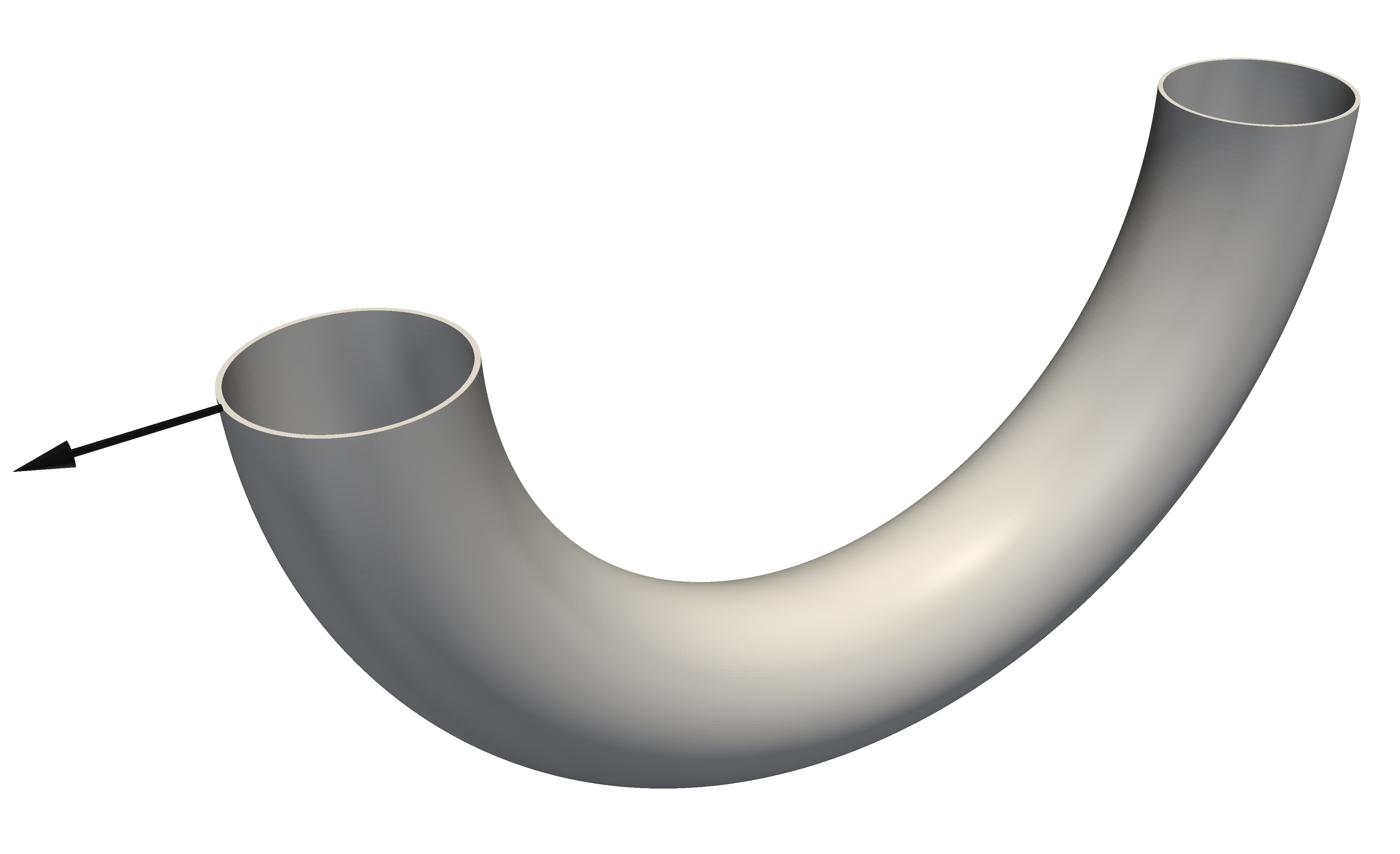
(a) Undeformed tube

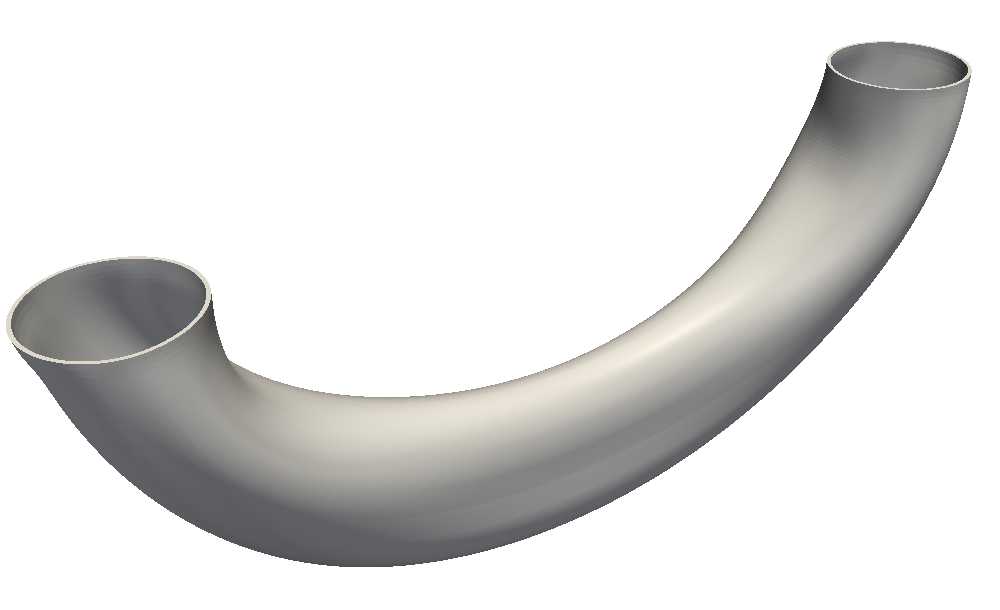
(b) Deformed tube

Figure 9: Deformation of an aluminum tube, modeled using a Neo-Hookean material model. The arrow represent the direction and magnitude of the displacement imposed as a boundary condition on the left end while the right end is kept fixed.

4.2 Time-dependent Problems

The following three examples discretize time-dependent, nonlinear problems. We first detail our solution strategy for these problems. For simplicity, we consider a scalar problem. We seek to find $\dot{u},u\in\mathcal{U}$ such that

$$\mathcal{R}(w;\dot{u},u)=0\quad\forall w\in\mathcal{W},$$

where $\mathcal{R}$ is a time-dependent, nonlinear residual functional.

We first use a semi-discrete approach by discretizing $\dot{u},u$ in space with finite-dimensional subspaces $\mathcal{U}^{h}\subset\mathcal{U}$, leaving the problem continuous in time. The span of the set of basis functions $\{N_{B}(\boldsymbol{x})\}_{B=0\dots n}$, $\boldsymbol{x}\in\Omega$ define the subspace $\mathcal{U}^{h}$. Similarly, we choose $\mathcal{W}^{h}\subset\mathcal{W}$ where $\text{span}\left(\{N_{A}(\boldsymbol{x})\}_{A=0\dots n-1}\right)$ defines $\mathcal{W}^{h}$. Given two sequences of time-dependent coefficients $\{\dot{U}_{B}(t)\},\{U_{B}(t)\}$, discrete functions $\dot{u}^{h},u^{h}$ are defined as

$$\dot{u}^{h}(\boldsymbol{x},t) =\sum_{B}\dot{U}_{B}(t)N_{B}(\boldsymbol{x}),$$

$$u^{h}(\boldsymbol{x},t) =\sum_{B}U_{B}(t)N_{B}(\boldsymbol{x}).$$

Denoting $\mathbf{\dot{U}}=\{\dot{U}_{B}(t)\},\mathbf{U}=\{U_{B}(t)\}$, we can write the residual vector,

$$\mathbf{R}\left(\mathbf{\dot{U}},\mathbf{U}\right)=\{R_{A}\},$$

where

$$R_{A}=\mathcal{R}\left(N_{A};\dot{u}^{h},u^{h}\right).$$

Next, we discretize in time using the generalized-$\alpha$ method for first order systems [57]. Given $\mathbf{\dot{U}}_{n},\mathbf{U}_{n}$, we seek $\mathbf{\dot{U}}_{n+1},\mathbf{U}_{n+1}$ such that

$$\mathbf{R}\left(\dot{\mathbf{U}}_{n+\alpha_{m}},\mathbf{U}_{n+\alpha_{f}}\right) =0$$ (27)

$$\mathbf{\dot{U}}_{n+\alpha_{m}} =\mathbf{\dot{U}}_{n}+\alpha_{m}\left(\mathbf{\dot{U}}_{n+1}-\mathbf{\dot{U}}_{n}\right)$$ (28)

$$\mathbf{U}_{n+\alpha_{f}} =\mathbf{U}_{n}+\alpha_{f}\left(\mathbf{U}_{n+1}-\mathbf{U}_{n}\right)$$ (29)

$$\mathbf{U}_{n+1} =\mathbf{U}_{n}+\Delta t\left(\gamma\dot{\mathbf{U}}_{n+1}+(1-\gamma)\dot{\mathbf{U}}_{n}\right)$$ (30)

where $\Delta t=t_{n+1}-t_{n}$ is the time step, and $\alpha_{f},\alpha_{m},\gamma$ are parameters which define the method. The generalized-$\alpha$ method was designed to filter (damp) high-frequency modes of the solution which are under-approximated. As opposed to linear problems, low and high frequency modes interact in nonlinear problems. Spurious high frequency modes lead to contamination of the resolved modes of the problem. The method parameters $\alpha_{f},\alpha_{m},\gamma$ can be chosen using the spectral radius $\rho_{\infty}\in[0,1]$ of the amplification matrix as $\Delta t\rightarrow\infty$ by

$$\alpha_{m} =\frac{1}{2}\left(\frac{3-\rho_{\infty}}{1+\rho_{\infty}}\right)$$

$$\alpha_{f} =\frac{1}{1+\rho_{\infty}}$$

$$\gamma =\frac{1}{2}+\alpha_{m}-\alpha_{f}$$

which leads to a second order, unconditionally stable method. The value of $\rho_{\infty}$ uniquely defines the method and can be chosen to filter a desired amount of high frequency modes.

In our experience, when approaching time-dependent, nonlinear problems, the generalized-$\alpha$ method is effective. The impact of the interaction of low and high frequency modes is problem dependent and not something necessarily understood in advance. In the case where no filtering is needed ($\rho_{\infty}=1$), the generalized-$\alpha$ method reduces to the implicit midpoint rule. Due to the popularity of the generalized-$\alpha$ method particularly among researchers in the isogeometric community, we have added it to PETSc’s time stepping algorithms and is available independently of the PetIGA framework. In the examples that follow, we solve equation (27) iteratively using Newton’s method, which requires the computation of the Jacobian of the residual vector at each iteration.

4.2.1 Cahn–Hilliard Equation

The Cahn–Hilliard equation governs the evolution of a binary mixture undergoing the process of phase separation. Let $\Omega\in\mathbb{R}^{d}$ be an open set, where $d=2,3$. The boundary of $\Omega$ with unit outward normal $\boldsymbol{n}$ is denoted $\Gamma$ and is composed of two complementary parts $\Gamma_{g}$ and $\Gamma_{h}$. Denoting $c$ the concentration of one of the components of the mixture, the problem can be stated in strong form as: find $c:\overline{\Omega}\times(0,T)\mapsto\mathbb{R}$ such that

$$\dfrac{\partial c}{\partial t}-\nabla\cdot\left(M_{c}\nabla\left(\mu_{c}-\lambda\Delta{c}\right)\right) =0\quad \Omega\times(0,T),$$ in

$$c =g \Gamma_{g}\times(0,T),$$ on

$$M_{c}\nabla\left(\mu_{c}-\lambda\Delta{c}\right)\cdot\boldsymbol{n} =h \Gamma_{h}\times(0,T),$$ on

$$M_{c}\lambda\nabla c\cdot\boldsymbol{n} =0 \Gamma\times(0,T),$$ on

$$c\left(\boldsymbol{x},0\right) =c_{0}\left(\boldsymbol{x}\right)\quad \overline{\Omega},$$ in

where $c_{0}$ is the initial concentration, $M_{c}$ is the mobility, $\mu_{c}$ represents the chemical potential of a binary mixture in the absence of phase interfaces, and $\lambda$ is a positive constant such that $\sqrt{\lambda}$ represents a length scale of the problem related to the interface thickness between the two phases. The mobility and chemical potential are nonlinear functions of the concentration

$$M_{c} =Dc(1-c),$$

$$\mu_{c} =\dfrac{1}{2\theta}\log\dfrac{c}{1-c}+1-2c,$$

in which $D$ is a positive constant with dimensions of diffusivity and $\theta$ is a dimensionless number which represents the ratio between critical and absolute temperatures.

We solve the Cahn–Hilliard equation in dimensionless form and with periodic boundary conditions as detailed in [7]. We show snapshots of the isocontours of the solution in three dimensions at different times during the simulation in figure 10.

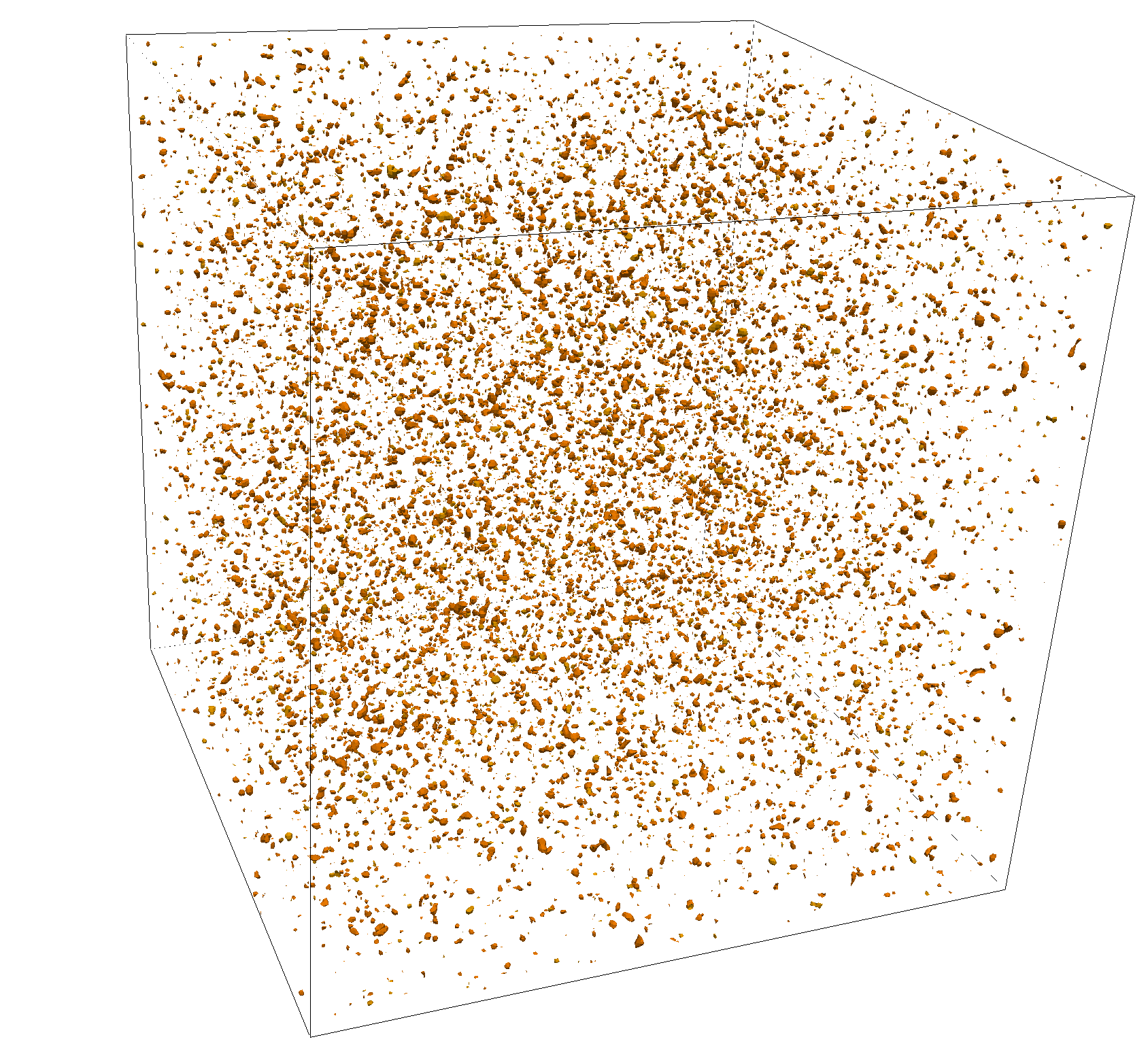
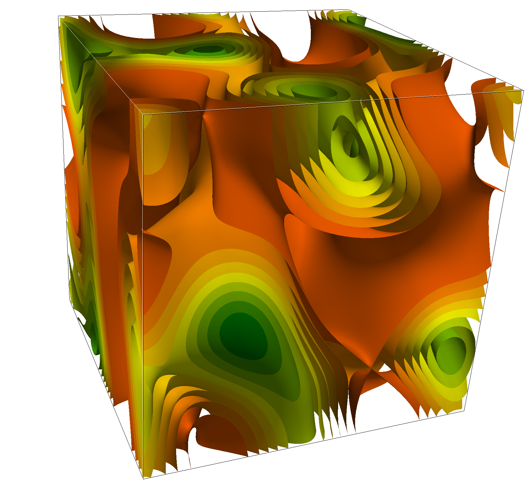
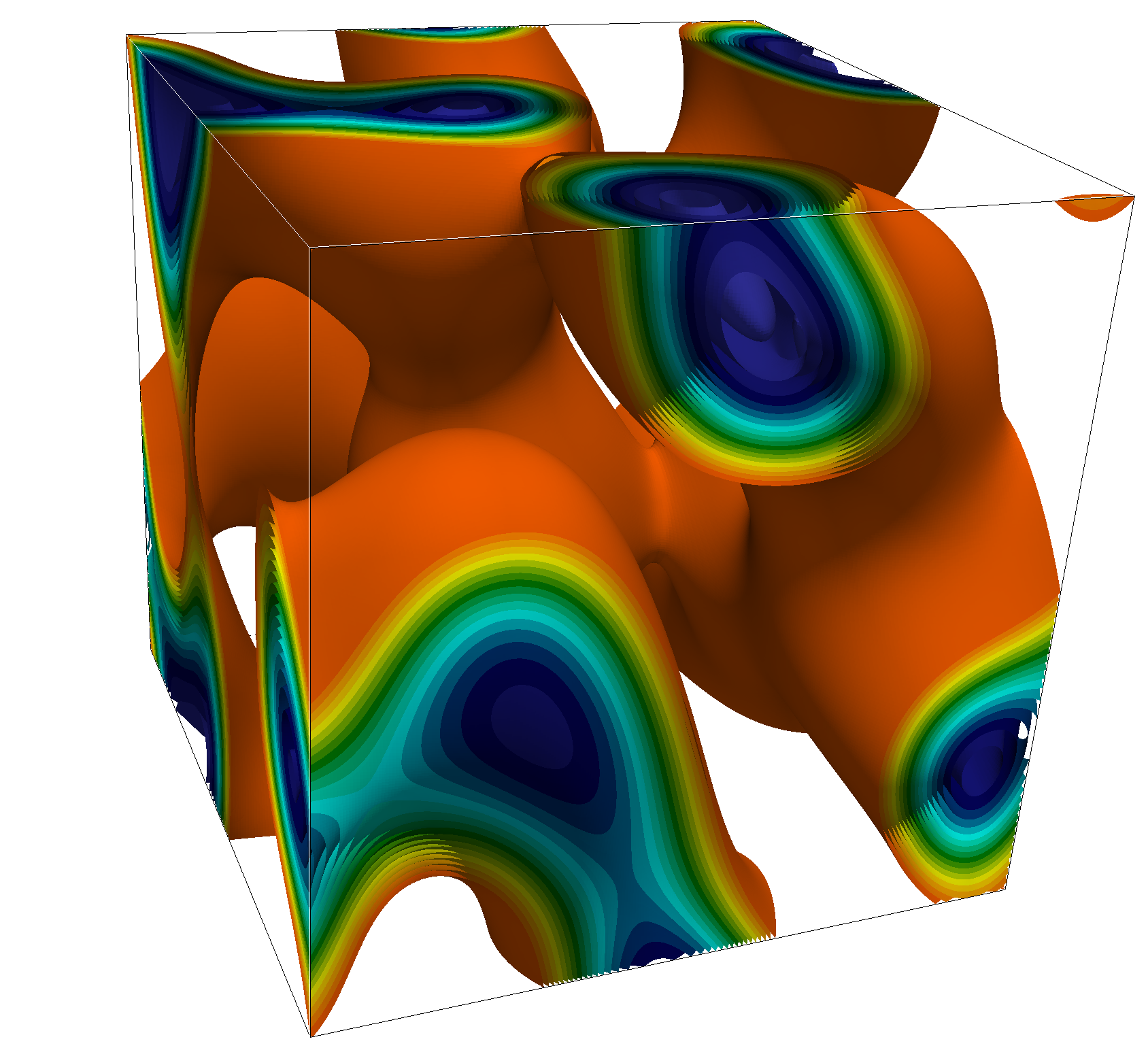
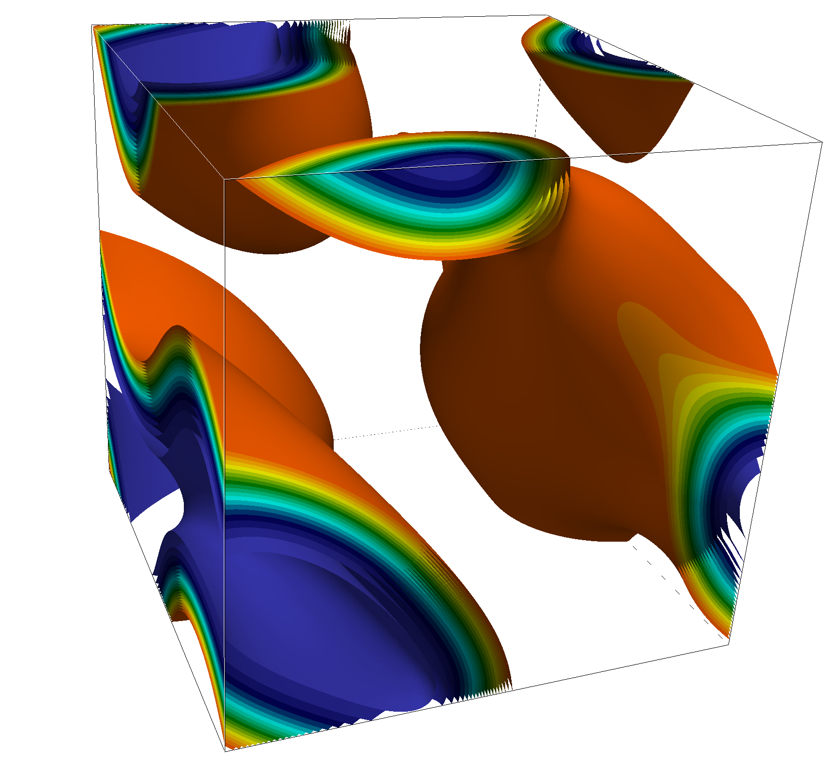
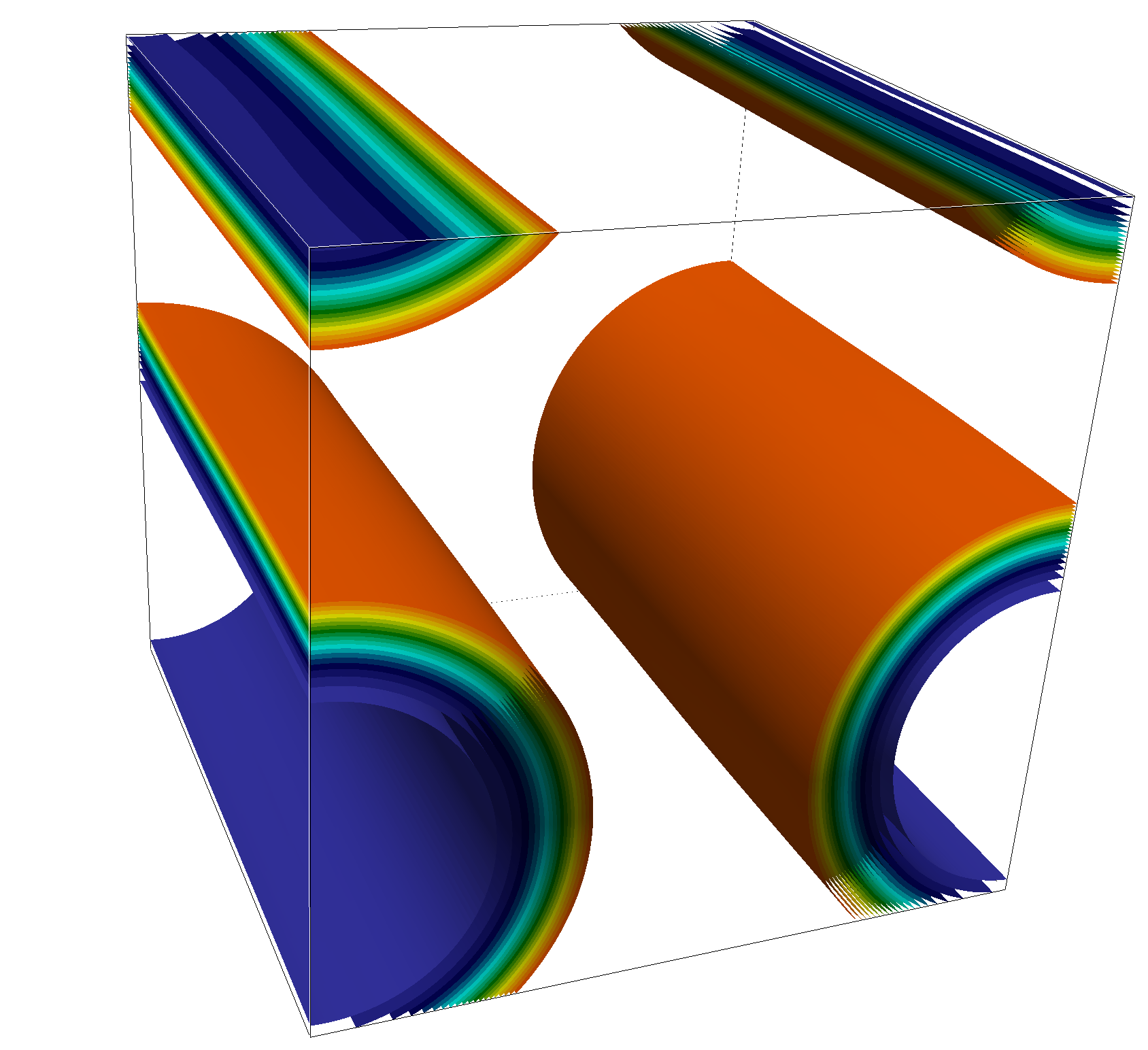
Figure 10: Transient solution to the Cahn–Hilliard problem in three dimensions, subject to a random initial condition and periodic boundary conditions. The weak form is discretized in space by a mesh of $256^{3}$ elements of $C^{1}$ quadratic B-splines.

4.2.2 Navier–Stokes–Korteweg Equations

The Navier–Stokes–Korteweg equations are a phase-field model for water and water vapor two-phase flows. Let $\Omega\in\mathbb{R}^{d}$ be an open set, where $d=2,3$. The boundary of $\Omega$ with unit outward normal $\boldsymbol{n}$ is denoted $\Gamma$. The problem can be stated in strong form as: find the density $\rho:\overline{\Omega}\times(0,T)\mapsto(0,b)$ and the velocity $\boldsymbol{u}:\overline{\Omega}\times(0,T)\mapsto\mathbb{R}^{d}$ such that

$$\dfrac{\partial\rho}{\partial t}+\nabla\cdot\left(\rho\boldsymbol{u}\right) =0\quad \Omega\times(0,T),$$ in

$$\dfrac{\partial\left(\rho\boldsymbol{u}\right)}{\partial t}+\nabla\cdot\left(\rho\boldsymbol{u}\otimes\boldsymbol{u}+p\boldsymbol{I}\right)-\nabla\cdot\boldsymbol{\tau}-\nabla\cdot\boldsymbol{\zeta} =\rho\boldsymbol{f}\quad \Omega\times(0,T),$$ in

$$\boldsymbol{u} =\boldsymbol{0}\quad \Gamma\times(0,T),$$ on

$$\nabla\rho\cdot\boldsymbol{n} =0\quad \Gamma\times(0,T),$$ on

$$\rho\left(\boldsymbol{x},0\right) =\rho_{0}\left(\boldsymbol{x}\right)\quad \overline{\Omega},$$ in

$$\boldsymbol{u}\left(\boldsymbol{x},0\right) =\boldsymbol{u}_{0}\left(\boldsymbol{x}\right)\quad \overline{\Omega},$$ in

where $\boldsymbol{u}_{0}$ and $\rho_{0}$ are initial values of the density and velocity, respectively. The function $\boldsymbol{f}$ represents the body force per unit mass. The viscous stress tensor is given as

$$\boldsymbol{\tau}=\bar{\mu}\left(\nabla\boldsymbol{u}+\nabla^{T}\boldsymbol{u}\right)+\bar{\lambda}\nabla\cdot\boldsymbol{u}\boldsymbol{I}$$

where $\bar{\mu}$ and $\bar{\lambda}$ are the viscosity coefficients and $\boldsymbol{I}$ is the identity tensor. The Korteweg tensor is defined as

$$\boldsymbol{\zeta}=\lambda\left(\rho\Delta\rho+\frac{1}{2}\|\nabla\rho\|^{2}\right)\boldsymbol{I}-\lambda\nabla\rho\otimes\nabla\rho$$

where $\lambda$ is the capillarity coefficient. The pressure is given by the van der Waals equation

$$p=Rb\frac{\rho\theta}{b-\rho}-a\rho^{2},$$

where $a,b$ are constants, $R$ is the ideal gas constant, and $\theta$ is the temperature, which for the isothermal model is assumed to be constant.

We solve the three-bubble test problem as detailed in [8] and show here the density and magnitude of the velocity for a two-dimensional solution in figure 11 and a three-dimensional solution in figure 12.

(a) Density

(b) Velocity (magnitude)

Figure 11: Time evolution (left to right) of the density and the magnitude of the velocity for the isothermal NSK equations on the three bubble test case problem.

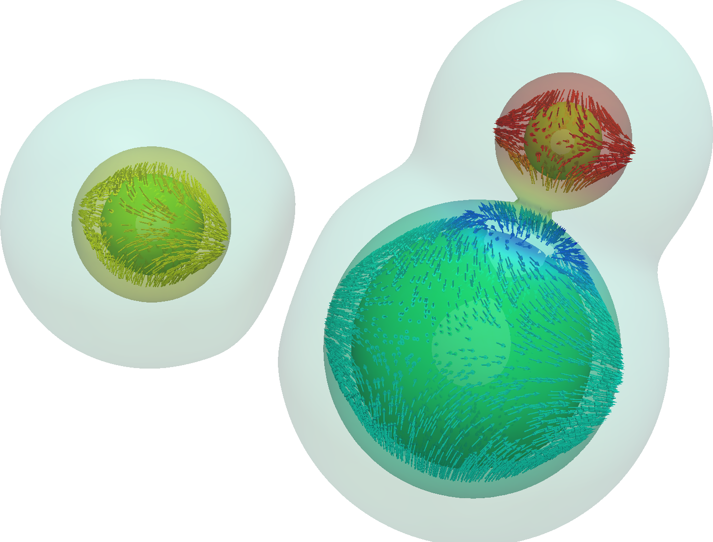
(a) Near the beginning of the simulation

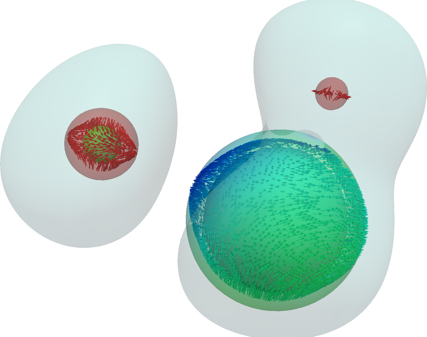
(b) Prior to the collapse of a bubble

Figure 12: Three-dimensional version of the three bubble problem for the Navier–Stokes–Korteweg equation. Isocontour surfaces reflect density values $\rho=\{0.15,0.55\}$ revealing the location of the three bubbles. Velocity vectors are shown on each isocontour and are colored by the velocity magnitude.

4.2.3 Navier–Stokes Equations

We solve the incompressible Navier–Stokes equations stabilized with the variational multiscale method as formulated in [58]. Let $\Omega\in\mathbb{R}^{d}$ be an open set, where $d=2,3$. The boundary of $\Omega$ with unit outward normal $\boldsymbol{n}$ is denoted $\Gamma$. The problem can be stated in strong form as: find the velocity $\boldsymbol{u}:\overline{\Omega}\times(0,T)\mapsto\mathbb{R}^{d}$ and the pressure (divided by the constant density) $p:\overline{\Omega}\times(0,T)\mapsto(0,b)$ such that

$$\dfrac{\partial\boldsymbol{u}}{\partial t}+\nabla\cdot\left(\boldsymbol{u}\otimes\boldsymbol{u}\right)+\nabla p =\nu\Delta\boldsymbol{u}+\boldsymbol{f}\quad \Omega\times(0,T),$$ in

$$\nabla\cdot\boldsymbol{u} =0\quad \Omega\times(0,T),$$ in

$$\boldsymbol{u} =\boldsymbol{0}\quad \Gamma\times(0,T),$$ on

$$\boldsymbol{u}\left(\boldsymbol{x},0\right) =\boldsymbol{u}_{0}\left(\boldsymbol{x}\right) \overline{\Omega},$$ in

where $\boldsymbol{u}_{o}$ is the initial velocity, $\boldsymbol{f}$ represents the body force per unit volume, and $\nu$ is the kinematic viscosity.

We solve a turbulent flow in a concentric pipe as presented in [59] the results of which we plot in figure 13. The domain is periodic in the streamwise direction. No-slip boundary conditions are set at the inner and outer cylinder surfaces and the initial condition is set using a laminar flow profile. The simulation is forced using a pressure gradient in the form of a body force in the streamwise direction.

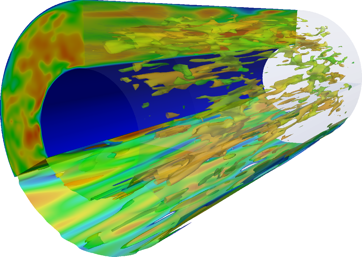
(a) Perspective view

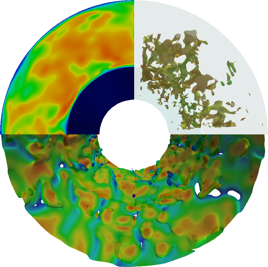
(b) Front view

Figure 13: Turbulent flow through concentric cylinders as in [59]. The top-left quadrant is a pseudocolor plot of the streamwise velocity. The top-right quadrant shows isocontours of the vorticity magnitude for smaller values. The bottom quadrants shows isocontours of the vorticity magnitude for larger values. Both sets of contours are colored by the streamwise velocity.

5 Performance

In this section we present scaling results of our code framework, applied to the incompressible Navier–Stokes equations described in section 4. Scaling of time-dependent, nonlinear problems can be difficult to quantify as solver component performance changes with problem size and decomposition. The nonlinearity increases slightly with the problem size, which can lead to extra Newton iterations for larger problems. The condition number of the linear system increases considerably with the size of the problem, requiring more linear iterations for convergence. At the same time, domain-decomposition-based preconditioners become weaker as more processors are employed, further increasing the number of iterations required by the linear solver.

With the goal of measuring the performance of the code while disregarding the algorithmic issues mentioned above, we perform tests with the following assumptions and constraints

• The problem is the flow between two plates problem with no-slip boundary conditions at the plate walls.

• The initial condition is set to the steady-state laminar flow profile.

• We discretize the domain using $C^{1}$ quadratic B-splines and employ full Gauss–Legendre quadrature with three quadrature points per direction on each element.

• We limit the test problem to ten time steps.

• We enforce the use of two nonlinear Newton iterations per time step.

• We enforce the use of $30$ GMRES iterations per Newton iteration.

• The preconditioner is block Jacobi with one block per process. and ILU(0) (incomplete LU factorization with zero fill-in) in each block.

We ran these tests on Stampede [60], a distributed memory supercomputing system featuring compute nodes with 2 $\times$ 8-core Intel Xeon E5-2680 (Sandy Bridge) processors, 32 GB of memory per node, and a InfiniBand Mellanox interconnect. In figure 14a and table 1, we show strong scaling and efficiency of the Navier–Stokes code on a single node using different discretization sizes indicated by the number of elements used, $n_{el}$. In figure 14b and table 2, we show strong scaling and efficiency on multiple compute nodes. In these multiple node runs, the parallel efficiency surpasses 80%, and is above 90% in all but one of the cases. These values are achieved for local problem sizes as small as $512$ elements per core.

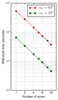
(a) Single node runs.

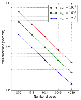
(b) Multiple node runs.

Figure 14: Strong scaling on Stampede. Wall-clock times corresponds to runs of the Navier–Stokes problem described in section 4. Each run spans ten time steps with a fixed number of Newton and GMRES iterations.

Table 1: Parallel efficiency on a single node of Stampede.

	Number of cores
Mesh	$1$	$2$	$4$	$6$	$8$	$12$	$16$
$n_{el}=32^{3}$	$100\%$	$98\%$	$95\%$	$90\%$	$90\%$	$89\%$	$91\%$
$n_{el}=64^{3}$	$100\%$	$94\%$	$92\%$	$90\%$	$90\%$	$86\%$	$89\%$

Table 2: Parallel efficiency on multiple nodes of Stampede.

	Number of cores
Mesh	$256$	$512$	$1024$	$2048$	$4096$
$n_{el}=128^{3}$	$100\%$	$99\%$	$97\%$	$94\%$	$85\%$
$n_{el}=160^{3}$	$100\%$	$99\%$	$97\%$	$96\%$	$92\%$
$n_{el}=192^{3}$	$100\%$	$98\%$	$95\%$	$95\%$	$93\%$

6 Conclusions

In this paper we present PetIGA, a scalable implementation of isogeometric analysis for linear/nonlinear and static/transient problems. By being built on top of PETSc, the framework gives users a robust and versatile platform to solve partial differential equations. We show that the framework scales well on up to $4096$ cores on the Navier–Stokes problem, and is therefore well suited for large scale applications. Even though primarily conceived for distributed-memory computing environments, PetIGA is also able to extract excellent performance on nowadays shared memory multicore laptop and desktop computers. Our software is already being used by members of the community to tackle challenging problems related to parallel multifrontal direct solvers [61], fast multipole-based preconditioners for elliptic equations [62], multilevel Monte Carlo algorithms geared towards the approximation of stochastic models [63], fluid-structure interaction [64], and finite strain gradient elasticity [65].

Up to now, we focused on making single patch geometries run as efficiently as possible. Single patch geometries are certainly enough for a wide range of academic applications. However, support for multipatch geometries is a must to tackle more complex simulations. Still, extending our framework to support multiple patches while keeping all of its user-friendly features and parallel distributed memory capabilities is a nontrivial task that will be addressed in future work. A multi-field extension of PetIGA is being developed on top of the current implementation to handle discrete differential forms. Promising results have already been obtained using divergence- and integral-conforming spaces to solve the Navier–Stokes–Cahn–Hilliard equation [66].

Appendix A Higher-order spatial derivatives

The geometric mapping is computed using the isoparametric concept, that is,

$$\boldsymbol{x}(\boldsymbol{\xi})=\sum_{A}\boldsymbol{x}_{A}N_{A}(\boldsymbol{\xi}),$$ (31)

where $N_{A}$ was defined in (6) and $\boldsymbol{x}_{A}$ are the control point locations in physical space. Thus, the parametric derivatives of this mapping are

$$\boldsymbol{x}_{,\alpha} =\dfrac{\partial\boldsymbol{x}(\boldsymbol{\xi})}{\partial\xi_{\alpha}}=\sum_{A}\boldsymbol{x}_{A}N_{A,\alpha},$$ (32)

$$\boldsymbol{x}_{,\alpha\beta} =\dfrac{\partial\boldsymbol{x}(\boldsymbol{\xi})}{\partial\xi_{\alpha}\partial\xi_{\beta}}=\sum_{A}\boldsymbol{x}_{A}N_{A,\alpha\beta},$$ (33)

$$\boldsymbol{x}_{,\alpha\beta\gamma} =\dfrac{\partial\boldsymbol{x}(\boldsymbol{\xi})}{\partial\xi_{\alpha}\partial\xi_{\beta}\partial\xi_{\gamma}}=\sum_{A}\boldsymbol{x}_{A}N_{A,\alpha\beta\gamma}.$$ (34)

For simplicity, we write them in index notation as $x_{i,\alpha}$, $x_{i,\alpha\beta}$, and $x_{i,\alpha\beta\gamma}$. Denoting the inverse mapping as $\boldsymbol{\xi}(\boldsymbol{x})$, the first spatial derivatives can be computed by matrix inversion through the identity

$$\delta_{ij}=x_{i,\epsilon}\ \xi_{\epsilon,j},$$ (35)

where $\delta_{ij}$ is the Kronecker delta. By repeated differentiation, second and third spatial derivatives of the inverse mapping follow:

$$\xi_{\alpha,ij} =x_{m,\epsilon\mu}\ \xi_{\alpha,m}\ \xi_{\epsilon,i}\ \xi_{\mu,j}$$ (36)

$$\xi_{\alpha,ijk} =-x_{m,\epsilon\mu\omega}\ \xi_{\alpha,m}\ \xi_{\epsilon,i}\ \xi_{\mu,j}\ \xi_{\omega,k}$$

$$\quad-x_{m,\epsilon\mu}\left(\xi_{\alpha,mk}\ \xi_{\epsilon,i}\ \xi_{\mu,j}+\xi_{\alpha,m}\ \xi_{\epsilon,ik}\ \xi_{\mu,j}+\xi_{\alpha,m}\ \xi_{\epsilon,i}\ \xi_{\mu,jk}\right)$$ (37)

Finally, the first, second, and third spatial derivatives of the basis functions are

$$N_{A,i} =N_{A,\alpha}\ \xi_{\alpha,i}$$ (38)

$$N_{A,ij} =N_{A,\alpha\beta}\ \xi_{\alpha,i}\ \xi_{\beta,j}+N_{A,\alpha}\ \xi_{\alpha,ij}$$ (39)

$$N_{A,ijk} =N_{A,\alpha\beta\gamma}\ \xi_{\alpha,i}\ \xi_{\beta,j}\ \xi_{\gamma,k}$$

$$+N_{A,\alpha\beta}\left(\xi_{\alpha,ik}\ \xi_{\beta,j}+\xi_{\alpha,i}\ \xi_{\beta,jk}+\xi_{\alpha,ij}\ \xi_{\beta,k}\right)$$

$$+N_{A,\alpha}\ \xi_{\alpha,ijk}.$$ (40)

Appendix B Tutorial for the Bratu example

This section complements section 3. It is meant as a tutorial that focuses on building and running codes using PETSc and PetIGA. In the following, we assume a POSIX environment such as GNU/Linux or OS X. Additionally, we assume that PETSc and PetIGA have been properly configured and built with an MPI implementation to enable parallel usage. As the usage of batch systems and job schedulers is quite specific to the distributed-memory computing environment users have access to, we only showcase parallel execution within a single compute node or desktop/laptop computer.

We set environment variables pointing to the PETSc and PetIGA directories as well as the PETSc build configuration. For recurrent use, these variables can be defined in the shell configuration file. When using the Bash shell, these definitions can be done as follows

$ export PETSC_DIR=/path/to/petsc
$ export PETSC_ARCH=arch-platform-c-opt
$ export PETIGA_DIR=/path/to/petiga

The ls command produces a listing with the content of the current working directory

$ ls -lh
-rw-rw-r--. 1 user users 1.7K Dec 31 23:58 Bratu.c
-rw-rw-r--. 1 user users  242 Dec 31 23:58 makefile

The Bratu.c file contains the C source code of the example under consideration. This code is available at the end of this section, see listing 1. The contents of makefile can be inspected with the cat command

$ cat makefile
Bratu: Bratu.PETIGA;
include $(PETIGA_DIR)/lib/petiga/conf/variables
include $(PETIGA_DIR)/lib/petiga/conf/rules

This makefile is simple: the first line defines a single target and the following two lines include variable definitions and build rules found within the PetIGA directory.

We use the make command to build the example. For the sake of brevity, we omit the verbose output from the compiler and linker. We then use the ls command once again to verify that the Bratu binary executable has indeed been generated

$ make Bratu
...
$ ls -lh
-rwxrwxr-x. 1 user users 146K Dec 31 23:59 Bratu
-rw-rw-r--. 1 user users 1.7K Dec 31 23:58 Bratu.c
-rw-rw-r--. 1 user users  242 Dec 31 23:58 makefile

Finally, we run the Bratu binary in parallel using four processes using the mpiexec command. Additionally, we pass some command line options to the program

$ mpiexec -n 4 ./Bratu -iga_elements 128 -iga_view -snes_monitor -ksp_type cg
IGA: dim=2 dof=1 order=2 geometry=0 rational=0 property=0
Axis 0: basis=BSPLINE[2,1] rule=LEGENDRE[3] periodic=0 nnp=130 nel=128
Axis 1: basis=BSPLINE[2,1] rule=LEGENDRE[3] periodic=0 nnp=130 nel=128
Partition - MPI: processors=[2,2,1] total=4
Partition - nnp: sum=16900 min=4096 max=4356 max/min=1.06348
Partition - nel: sum=16384 min=4096 max=4096 max/min=1
  0 SNES Function norm 5.266384548611e-02
  1 SNES Function norm 8.620220401724e-03
  2 SNES Function norm 2.054605014212e-03
  3 SNES Function norm 4.716226279209e-04
  4 SNES Function norm 8.916608064674e-05
  5 SNES Function norm 8.438014748365e-06
  6 SNES Function norm 1.155533195923e-07
  7 SNES Function norm 2.309601078808e-11

The option -iga_view displays various details related to the discretization and parallel partitioning. From the first output line, we verify the problem is two-dimensional and the solution has a single component. The second and third line provide information about the discretization along each direction: the problem is being solved in a grid with $128{\times}128$ elements (as requested through the -iga_elements option), quadratic $C^{1}$ B-spline basis functions, and Gauss–Legendre quadrature with three points per direction. The option -snes_monitor monitors the nonlinear solver convergence by printing the iteration number and the 2-norm of the global residual vector. Finally, the option -ksp_type configures the linear solver to use the conjugate gradient method. Many more options are available to control the nonlinear solver, the linear solver, and the preconditioner. These options can be listed by passing the -help option.

Thanks to the call to the VecViewFromOptions routine, we visualize the solution at runtime

$ mpiexec -n 4 ./Bratu -iga_elements 128 -output draw:x -draw_pause 5

This feature allows users to quickly check for a sensible solution, as seen in figure 15a. This is particularly useful while in the initial setup of a time-dependent problem. To obtain higher quality visualizations, the option value can be changed to dump a VTK file to disk, which can then be post-processed with tools such as ParaView [70], as seen in figure 15b.

$ mpiexec -n 4 ./Bratu -iga_elements 128 -output vtk:Bratu.vts
$ ls -lh Bratu.vts
-rw-rw-r--. 1 user users 2.1M Jan  1 00:01 Bratu.vts
$ paraview Bratu.vts

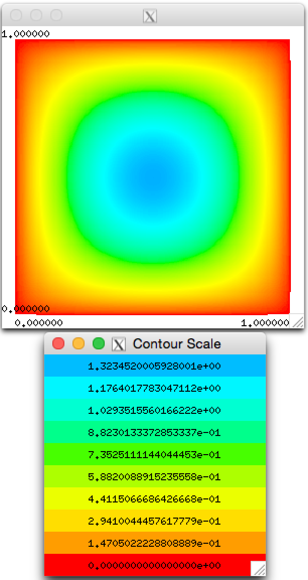
(a) Visualizing at runtime.

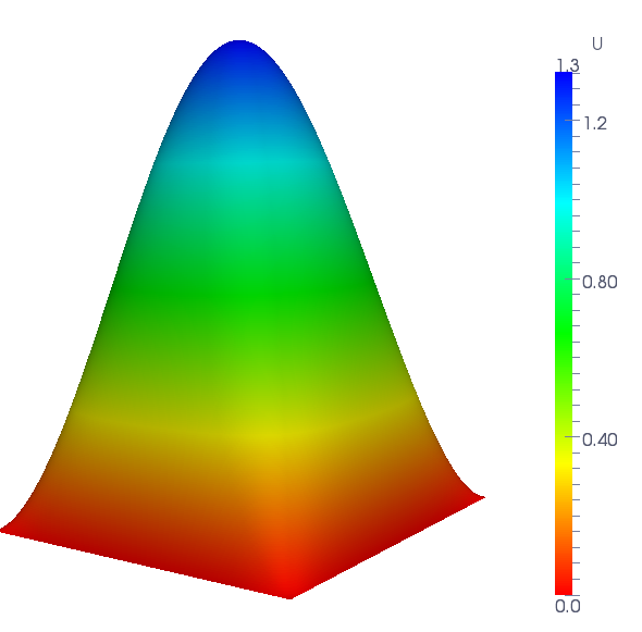
(b) Post-processing with ParaView.

Figure 15: Visualizing the solution of the Bratu equation.

Listing 1: C source code for the Bratu example

⬇

#include <petiga.h>

#define dim 2

#define dot(a,b) (a[0]*b[0]+a[1]*b[1])

typedef struct {

double lambda;

} Params;

int Residual(IGAPoint p,const double U[],double R[],void *ctx) {

int a,nen = p->nen;

double (*N0) = (typeof(N0)) p->shape[0];

double (*N1)[dim] = (typeof(N1)) p->shape[1];

double u,grad_u[dim],lambda = ((Params*)ctx)->lambda;

IGAPointFormValue(p,U,&u);

IGAPointFormGrad (p,U,grad_u);

for (a=0; a<nen; a++)

R[a] = dot(N1[a],grad_u) - lambda*exp(u)*N0[a];

return 0;

}

int Jacobian(IGAPoint p,const double U[],double J[],void *ctx) {

int a,b,nen = p->nen;

double (*N0) = (typeof(N0)) p->shape[0];

double (*N1)[dim] = (typeof(N1)) p->shape[1];

double u,lambda = ((Params*)ctx)->lambda;

IGAPointFormValue(p,U,&u);

for (a=0; a<nen; a++)

for (b=0; b<nen; b++)

J[a*nen+b] = dot(N1[a],N1[b]) - lambda*exp(u)*N0[a]*N0[b];

return 0;

}

int main(int argc, char *argv[]) {

PetscInitialize(&argc,&argv,NULL,NULL);

IGA iga;

IGACreate(PETSC_COMM_WORLD,&iga);

IGASetDim(iga,dim);

IGASetDof(iga,1);

IGASetFromOptions(iga);

IGASetUp(iga);

int direction,side;

for (direction=0; direction<dim; direction++) {

for (side=0; side<2; side++) {

int field = 0; double value = 0.0;

IGASetBoundaryValue(iga,direction,side,field,value);

}

}

Params params;

params.lambda = IGAGetOptReal(NULL,"-lambda",6.80);

IGASetFormFunction(iga,Residual,&params);

IGASetFormJacobian(iga,Jacobian,&params);

SNES snes;

IGACreateSNES(iga,&snes);

SNESSetFromOptions(snes);

Vec U;

IGACreateVec(iga,&U);

SNESSolve(snes,NULL,U);

VecViewFromOptions(U,NULL,"-output");

VecDestroy(&U);

SNESDestroy(&snes);

IGADestroy(&iga);

PetscFinalize();

return 0;

}

Appendix C Numerical differentiation comparison

In this section we present some benchmark results measuring the computational overhead of two numerical differentiation approaches discussed in section 2.8. We base our tests on the Bratu problem described in section 3. However, we now focus on the three-dimensional counterpart to make the problem more computationally challenging. We use a modified version of the code listing 1 presented in appendix B: instead of solving the nonlinear problem, we compute the global Jacobian matrix and report the minimum wall clock time from five successive computations. These computations are performed with three different methods.

• Explicit uses the explicitly coded, user-provided Jacobian routine, as described in section 3,

• Coloring uses the global colored finite differences implementation available in PETSc,

• Local ND uses the local (i.e., at quadrature points) numerical differentiation implementation available in PetIGA.

The benchmarks where run in a workstation with two Intel Xeon CPU E5-2680 v2 (10 cores, 2.80GHz, 25 MB cache, 8 GT/s QPI) and 128 GB of memory running Linux 4.0.4 (Fedora 21) and used the in-development versions of PETSc and PetIGA compiled with GCC 4.9.2 using the -Ofast optimization flag.

The benchmark results are summarized in table 3. Parameters $P$, $n_{el}$, $p$, and $k$ refer to number of processes, number of elements, degree and continuity order of the polynomial space, respectively. All cases used full Gauss–Legendre quadrature with $p+1$ quadrature points per direction. Taking the explicitly coded Jacobian computations as a baseline, colored finite differences is over an order of magnitude slower whereas the local numerical differentiation approach is only about four times slower.

Table 3: Benchmark of numerical differentiation schemes. Parameters $P$ and $n_{el}$ denote number of processes and elements, respectively, while $p$ and $k$ denote polynomial degree and continuity order, respectively. We report the minimum wall clock time from five successive computations of the global Jacobian matrix corresponding to the 3D Bratu problem.

				Time (seconds)
$P$	$n_{el}$	$p$	$k$	Explicit	Coloring	Local ND
		2	0	$0.31$	$7.67$	$1.21$
8	$32^{3}$		1	$0.33$	$7.79$	$1.24$
		3	2	$3.71$	$105.08$	$15.27$
		2	0	$1.31$	$34.44$	$5.15$
	$64^{3}$		1	$1.35$	$34.84$	$5.26$
16		3	2	$15.41$	$452.67$	$64.93$
	$128^{3}$	1	0	$0.52$	$10.35$	$1.72$
		2	1	$10.74$	$307.06$	$41.46$

references.0references.0ReferencesReferencesreferences.0

References

- [1] T.J.R. Hughes, J.A. Cottrell, Y. Bazilevs, Isogeometric analysis: CAD, finite elements, NURBS, exact geometry and mesh refinement, Computer Methods in Applied Mechanics and Engineering 194 (39–41) (2005) 4135–4195. doi:10.1016/j.cma.2004.10.008.
- [2] J.A. Cottrell, T.J.R. Hughes, Y. Bazilevs, Isogeometric Analysis: Toward Unification of CAD and FEA, John Wiley & Sons, Ltd, 2009. doi:10.1002/9780470749081.
- [3] M. Bercovier, G. Berold, Solving design problems by integration of CAD and FEM software, in: B. Ford, F. Chatelin (Eds.), Proceedings of IFIP TC 2/WG 2.5 Working Conference on Problem Solving Environments for Scientific Computing, Sophia Antipolis, France, 17–21 June, 1985, North Holland, 1987, p. 309.
- [4] A. Sheffer, T. Blacker, M. Bercovier, Steps towards smooth CAD–FEM integration, in: Proceedings of 6th International Conference on Numerical Grid Generation in Computational Field Simulations, 1998, pp. 705–714.
- [5] A. Sheffer, M. Bercovier, CAD model editing and its applications, Ph.D. thesis, Hebrew University of Jerusalem (1999).
- [6] K. Höllig, Finite Element Methods with B-splines, Frontiers in Applied Mathematics, Society for Industrial and Applied Mathematics, 2003. doi:10.1137/1.9780898717532.
- [7] H. Gomez, V.M. Calo, Y. Bazilevs, T.J.R. Hughes, Isogeometric analysis of the Cahn–Hilliard phase-field model, Computer Methods in Applied Mechanics and Engineering 197 (49–50) (2008) 4333–4352. doi:10.1016/j.cma.2008.05.003.
- [8] H. Gomez, T.J.R. Hughes, X. Nogueira, V.M. Calo, Isogeometric analysis of the isothermal Navier–Stokes–Korteweg equations, Computer Methods in Applied Mechanics and Engineering 199 (25–28) (2010) 1828–1840. doi:10.1016/j.cma.2010.02.010.
- [9] P. Vignal, L. Dalcin, D.L. Brown, N. Collier, V.M. Calo, An energy-stable convex splitting for the phase-field crystal equation, Computers & Structures 158 (2015) 355––368. doi:10.1016/j.compstruc.2015.05.029.
- [10] D.J. Benson, Y. Bazilevs, M.-C. Hsu, T.J.R. Hughes, A large deformation, rotation-free, isogeometric shell, Computer Methods in Applied Mechanics and Engineering 200 (13–16) (2011) 1367–1378. doi:10.1016/j.cma.2010.12.003.
- [11] J. Kiendl, M.-C. Hsu, M.C.H. Wu, A. Reali, Isogeometric Kirchhoff–Love shell formulations for general hyperelastic materials, Computer Methods in Applied Mechanics and Engineering 291 (0) (2015) 280–303. doi:10.1016/j.cma.2015.03.010.
- [12] R. Bouclier, T. Elguedj, A. Combescure, An isogeometric locking–free NURBS-based solid–shell element for geometrically nonlinear analysis, International Journal for Numerical Methods in Engineering 101 (10) (2015) 774–808. doi:10.1002/nme.4834.
- [13] I. Akkerman, Y. Bazilevs, V.M. Calo, T.J.R. Hughes, S. Hulshoff, The role of continuity in residual-based variational multiscale modeling of turbulence, Computational Mechanics 41 (3) (2008) 371–378. doi:10.1007/s00466-007-0193-7.
- [14] I. Akkerman, Y. Bazilevs, C.E. Kees, M.W. Farthing, Isogeometric analysis of free-surface flow, Journal of Computational Physics 230 (11) (2011) 4137–4152, special issue High Order Methods for CFD Problems. doi:10.1016/j.jcp.2010.11.044.
- [15] A. Buffa, J. Rivas, G. Sangalli, R. Vázquez, Isogeometric discrete differential forms in three dimensions, SIAM Journal on Numerical Analysis 49 (2) (2011) 818–844. doi:10.1137/100786708.
- [16] J.A. Evans, T.J.R. Hughes, Isogeometric divergence-conforming B-splines for the unsteady Navier–Stokes equations, Journal of Computational Physics 241 (2013) 141–167. doi:10.1016/j.jcp.2013.01.006.
- [17] L. Beirão da Veiga, A. Buffa, J. Rivas, G. Sangalli, Some estimates for h–p–k-refinement in Isogeometric Analysis, Numerische Mathematik 118 (2011) 271–305. doi:10.1007/s00211-010-0338-z.
- [18] J.A. Evans, Y. Bazilevs, I. Babuška, T.J.R. Hughes, -Widths, sup–infs, and optimality ratios for the -version of the isogeometric finite element method, Computer Methods in Applied Mechanics and Engineering 198 (21–26) (2009) 1726–1741, advances in Simulation-Based Engineering Sciences – Honoring J. Tinsley Oden. doi:10.1016/j.cma.2009.01.021.
- [19] N. Collier, L. Dalcin, V.M. Calo, On the computational efficiency of isogeometric methods for smooth elliptic problems using direct solvers, International Journal for Numerical Methods in Engineering 100 (8) (2014) 620–632. doi:10.1002/nme.4769.
- [20] N. Collier, D. Pardo, L. Dalcin, M. Paszynski, V.M. Calo, The cost of continuity: A study of the performance of isogeometric finite elements using direct solvers, Computer Methods in Applied Mechanics and Engineering 213–216 (2012) 353–361. doi:10.1016/j.cma.2011.11.002.
- [21] N. Collier, L. Dalcin, D. Pardo, V.M. Calo, The cost of continuity: Performance of iterative solvers on isogeometric finite elements, SIAM Journal on Scientific Computing 35 (2) (2013) A767–A784. doi:10.1137/120881038.
- [22] R. Baxter, N.C. Hong, D. Gorissen, J. Hetherington, I. Todorov, The research software engineer, in: Digital Research Conference, Oxford, 2012, pp. 1–3.
- [23] G. Wilson, Those who will not learn from history…, Computing in Science & Engineering 10 (3) (2008) 5–6. doi:10.1109/MCSE.2008.86.
-
[24]
S. Balay, S. Abhyankar, M.F. Adams, J. Brown, P. Brune, K. Buschelman,
L. Dalcin, V. Eijkhout, W.D. Gropp, D. Kaushik, M.G. Knepley, L. Curfman
McInnes, K. Rupp, B.F. Smith, S. Zampini, H. Zhang.
PETSc Web page [online]
(2015).
URL http://www.mcs.anl.gov/petsc -
[25]
S. Balay, S. Abhyankar, M.F. Adams, J. Brown, P. Brune, K. Buschelman,
L. Dalcin, V. Eijkhout, W.D. Gropp, D. Kaushik, M.G. Knepley, L. Curfman
McInnes, K. Rupp, B.F. Smith, S. Zampini, H. Zhang,
PETSc
users manual, Tech. Rep. ANL-95/11 - Revision 3.6, Argonne National
Laboratory (2015).
URL http://www.mcs.anl.gov/petsc/petsc-current/docs/manual.pdf - [26] S. Balay, W.D. Gropp, L. Curfman McInnes, B.F. Smith, Efficient management of parallelism in object oriented numerical software libraries, in: E. Arge, A.M. Bruaset, H.P. Langtangen (Eds.), Modern Software Tools in Scientific Computing, Birkhäuser Press, 1997, pp. 163–202.
- [27] R.D. Falgout, U.M. Yang, hypre: A library of high performance preconditioners, in: P.M.A. Sloot, A.G. Hoekstra, C.J. Kenneth Tan, J.J. Dongarra (Eds.), Computational Science – ICCS 2002, Vol. 2331 of Lecture Notes in Computer Science, Springer Berlin Heidelberg, 2002, pp. 632–641. doi:10.1007/3-540-47789-6_66.
- [28] M.A. Heroux, R.A. Bartlett, V.E. Howle, R.J. Hoekstra, J.J. Hu, T.G. Kolda, R.B. Lehoucq, K.R. Long, R.P. Pawlowski, E.T. Phipps, A.G. Salinger, H.K. Thornquist, R.S. Tuminaro, J.M. Willenbring, A. Williams, K.S. Stanley, An overview of the Trilinos project, ACM Transactions on Mathematical Software 31 (3) (2005) 397–423. doi:10.1145/1089014.1089021.
- [29] P.R. Amestoy, A. Guermouche, J.-Y. L’Excellent, S. Pralet, Hybrid scheduling for the parallel solution of linear systems, Parallel Computing 32 (2) (2006) 136–156, parallel Matrix Algorithms and Applications. doi:10.1016/j.parco.2005.07.004.
- [30] W. Bangerth, R. Hartmann, G. Kanschat, deal.II – a general purpose object oriented finite element library, ACM Transactions on Mathematical Software 33 (4) (2007) 24/1–24/27. doi:10.1145/1268776.1268779.
- [31] A. Logg, K.-A. Mardal, G. Wells, Automated Solution of Differential Equations by the Finite Element Method, Springer Berlin Heidelberg, 2012.
- [32] B.S. Kirk, J.W. Peterson, R.H. Stogner, G.F. Carey, libMesh: A C++ Library for Parallel Adaptive Mesh Refinement/Coarsening Simulations, Engineering with Computers 22 (3–4) (2006) 237–254. doi:10.1007/s00366-006-0049-3.
- [33] V.E. Sonzogni, A.M. Yommi, N.M. Nigro, M.A. Storti, A parallel finite element program on a beowulf cluster, Advances in Engineering Software 33 (7–10) (2002) 427–443, engineering Computational Technology & Computational Structures Technology. doi:10.1016/S0965-9978(02)00059-5.
-
[34]
L. Dalcin, N. Collier.
PetIGA: High
performance isogeometric analysis [online] (2015).
URL https://bitbucket.org/dalcinl/petiga - [35] M.G. Cox, The numerical evaluation of B-splines, IMA Journal of Applied Mathematics 10 (2) (1972) 134–149. doi:10.1093/imamat/10.2.134.
- [36] C. de Boor, On calculation with B-splines, Journal of Approximation Theory 6 (1) (1972) 50–62. doi:10.1016/0021-9045(72)90080-9.
- [37] L. Piegl, W. Tiller, The NURBS Book, Monographs in Visual Communication, Springer, 1995.
- [38] T.J.R. Hughes, The finite element method: linear static and dynamic finite element analysis, Dover Publications, 2000.
- [39] J. Liu, L. Dedè, J.A. Evans, M.J. Borden, T.J.R. Hughes, Isogeometric analysis of the advective Cahn-Hilliard equation: Spinodal decomposition under shear flow, Journal of Computational Physics 242 (2013) 321–350. doi:10.1016/j.jcp.2013.02.008.
- [40] D.A. Knoll, D.E. Keyes, Jacobian-free newton–krylov methods: a survey of approaches and applications, Journal of Computational Physics 193 (2) (2004) 357–397. doi:10.1016/j.jcp.2003.08.010.
- [41] A.H. Gebremedhin, F. Manne, A. Pothen, What color is your Jacobian? graph coloring for computing derivatives, SIAM Review 47 (4) (2005) 629–705. doi:10.1137/S0036144504444711.
- [42] M. Pernice, H. F. Walker, NITSOL: A Newton iterative solver for nonlinear systems, SIAM Journal on Scientific Computing 19 (1998) 302–318.
- [43] T.J.R. Hughes, A. Reali, G. Sangalli, Efficient quadrature for NURBS-based isogeometric analysis, Computer Methods in Applied Mechanics and Engineering 199 (5–8) (2010) 301–313.
- [44] R. Ait-Haddou, M. Bartoň, V.M. Calo, Explicit Gaussian quadrature rules for cubic splines with non-uniform knot sequences, ArXiv e-prints (2014) 1–15.arXiv:1410.7196.
- [45] M. Bartoň, R. Ait-Haddou, V.M. Calo, Gaussian quadrature rules for quintic splines, ArXiv e-prints (2015) 1–20.arXiv:1503.00907.
- [46] M. Bartoň, V.M. Calo, Gaussian quadrature for splines via homotopy continuation: rules for cubic splines, ArXiv e-prints (2015) 1–22.arXiv:1505.04391.
- [47] G.E. Karniadakis, S.J. Sherwin, Spectral/hp Element Methods for Computational Fluid Dynamics, 2nd Edition, Oxford University Press, 2013.
- [48] F. Auricchio, Beirão Da Veiga, T.J.R. Hughes, A. Reali, G. Sangalli, Isogeometric collocation methods, Mathematical Models and Methods in Applied Sciences 20 (11) (2010) 2075–2107. doi:10.1142/S0218202510004878.
-
[49]
L. Dalcin, N. Collier.
igakit [online] (2015).
URL https://bitbucket.org/dalcinl/igakit -
[50]
N. Collier, L. Dalcin.
PetIGA and igakit
tutorial [online] (2015).
URL https://petiga-igakit.readthedocs.org - [51] J. Jacobsen, K. Schmitt, The Liouville-Bratu-Gelfand Problem for Radial Operators, Journal of Differential Equations 184 (1) (2002) 283–298. doi:10.1006/jdeq.2001.4151.
- [52] W. Schroeder, K. Martin, B. Lorensen, The Visualization Toolkit, 4th edition, Kitware Inc., 2006.
- [53] VTK File Formats, www.vtk.org/VTK/img/file-formats.pdf (2015).
- [54] L.M. Bernal, V.M. Calo, N. Collier, G.A. Espinosa, F. Fuentes, J.C. Mahecha, Isogeometric analysis of hyperelastic materials using PetIGA, Procedia Computer Science 18 (0) (2013) 1604–1613, 2013 International Conference on Computational Science. doi:10.1016/j.procs.2013.05.328.
- [55] J.C. Simo, T.J.R. Hughes, Computational Inelasticity, Springer, 1998.
- [56] O. Gonzalez, A.M. Stuart, A First Course in Continuum Mechanics, Cambridge University Press, 2008.
- [57] K.E. Jansen, C.H. Whiting, G.M. Hulbert, A generalized- method for integrating the filtered Navier–Stokes equations with a stabilized finite element method, Computer Methods in Applied Mechanics and Engineering 190 (3–4) (2000) 305–319. doi:10.1016/S0045-7825(00)00203-6.
- [58] Y. Bazilevs, V.M. Calo, J.A. Cottrell, T.J.R. Hughes, A. Reali, G. Scovazzi, Variational multiscale residual-based turbulence modeling for large eddy simulation of incompressible flows, Computer Methods in Applied Mechanics and Engineering 197 (1–4) (2007) 173–201. doi:10.1016/j.cma.2007.07.016.
- [59] Y.G. Motlagh, H.T. Ahn, T.J.R. Hughes, V.M. Calo, Simulation of laminar and turbulent concentric pipe flows with the isogeometric variational multiscale method, Computers & Fluids 71 (2013) 146–155. doi:10.1016/j.compfluid.2012.09.006.
-
[60]
Texas Advanced Computing Center [online]
(2015).
URL http://www.tacc.utexas.edu/ - [61] M. Woźniak, K. Kuźnik, M. Paszyński, V.M. Calo, D. Pardo, Computational cost estimates for parallel shared memory isogeometric multi-frontal solvers, Computers & Mathematics with Applications 67 (10) (2014) 1864–1883. doi:10.1016/j.camwa.2014.03.017.
- [62] R. Yokota, J. Pestana, H. Ibeid, D. Keyes, Fast multipole preconditioners for sparse matrices arising from elliptic equations, Computing Research Repository (2014) 1–32.arXiv:1308.3339.
- [63] N. Collier, A-.L. Haji-Ali, F. Nobile, E. von Schwerin, R. Tempone, A continuation multilevel Monte Carlo algorithm, BIT Numerical Mathematics 55 (2) (2015) 399–432. doi:10.1007/s10543-014-0511-3.
- [64] H. Casquero, C. Bona-Casas, H. Gomez, A NURBS-based immersed methodology for fluid-structure interaction, Computer Methods in Applied Mechanics and Engineering 284 (0) (2015) 943–970, isogeometric Analysis Special Issue. doi:10.1016/j.cma.2014.10.055.
- [65] S. Rudraraju, A. Van der Ven, K. Garikipati, Three-dimensional isogeometric solutions to general boundary value problems of toupin’s gradient elasticity theory at finite strains, Computer Methods in Applied Mechanics and Engineering 278 (0) (2014) 705–728. doi:10.1016/j.cma.2014.06.015.
- [66] P. Vignal, A. Sarmiento, A.M.A. Côrtes, L. Dalcin, V.M. Calo, Coupling Navier-Stokes and Cahn-Hilliard equations in a two-dimensional annular flow configuration, Procedia Computer Science 51 (0) (2015) 934–943, international Conference On Computational Science, {ICCS} 2015 Computational Science at the Gates of Nature. doi:10.1016/j.procs.2015.05.228.
- [67] T.E. Oliphant, A Guide to NumPy, Trelgol Publishing, 2006.
- [68] J.D. Hunter, Matplotlib: A 2D graphics environment, Computing in Science & Engineering 9 (3) (2007) 90—95. doi:10.1109/MCSE.2007.55.
- [69] F. Pérez, B.E. Granger, IPython: a system for interactive scientific computing, Computing in Science & Engineering 9 (3) (2007) 21–29. doi:10.1109/MCSE.2007.53.
- [70] A. Henderson, ParaView guide, a parallel visualization application, Tech. Rep. Revision 4.1, Kitware Inc. (2014).