Self-trapping dynamics in a 2D optical lattice

Abstract

We describe theoretical models for the recent experimental observation of Macroscopic Quantum Self-Trapping (MQST) in the transverse dynamics of an ultracold bosonic gas in a 2D lattice. The pure mean-field model based on the solution of coupled nonlinear equations fails to reproduce the experimental observations. It greatly overestimates the initial expansion rates at short times and predicts a slower expansion rate of the cloud at longer times. It also predicts the formation of a hole surrounded by a steep square fort-like barrier which was not observed in the experiment. An improved theoretical description based on a simplified Truncated Wigner Approximation (TWA), which adds phase and number fluctuations in the initial conditions, pushes the theoretical results closer to the experimental observations but fails to quantitatively reproduce them. An explanation of the delayed expansion as a consequence of a new type of self-trapping mechanism, where quantum correlations suppress tunneling even when there are no density gradients, is discussed and supported by numerical time-dependent Density Matrix Renormalization Group (t-DMRG) calculations performed in a simplified two coupled tubes set-up.

I introduction

The term “self-trapping” was first introduced by Landau to describe the motion of an electron in a crystal lattice Landau (1933). According to Landau, the electron gets dressed by the lattice polarization and deformation caused by its own motion. The resulting polaron can be localized or self-trapped in the presence of strong electron-lattice interactions. Nowadays, the concept of self-trapped polarons is applied to various condensed matter systems such as semiconductors, organic molecular crystals, high temperature cuprate superconductors and colossal magnetoresistance manganates Shluger and Stoneham (1993); Salje et al. (1995); Millis et al. (1995). Still, the theory of the dynamical coupling of a conduction electron to lattice phonons is a complicated highly nonlinear problem which is difficult to tackle even in one-dimensional situations Wellein and Fehske (1998). Many questions remain open.

A parallel situation in which self-trapping has been theoretically investigated and experimentally observed is in dilute ultra-cold bosonic gases Milburn et al. (1997); Smerzi et al. (1997); Raghavan et al. (1999); Trombettoni and Smerzi (2001); Morsch et al. (2002); Smerzi and Trombettoni (2003); Albiez et al. (2005); Anker et al. (2005); Alexander et al. (2006); Xue et al. (2008); Wüster et al. (2012). In those systems, self trapping is caused by a competition between the discreteness introduced by the lattice and non-linear effects. However, in these systems the lattice potential is rigid, imposed by optical fields, and the non-linearity has its roots in intrinsic interatomic interactions. The self-trapping mechanism is then inherently a many-particle phenomenon, commonly referred to as Macroscopic Quantum Self -Trapping (MQST).

MQST has been experimentally observed with cold atoms in double well setups Albiez et al. (2005) and in 1D lattice geometries Anker et al. (2005). MQST can be understood as wave-packet localization caused by the interaction-induced suppression of tunneling in the presence of chemical potential gradients. In those cases, a mean field description in terms of the so called time-dependent Gross-Pitaevskii equation (GPE) is shown to be sufficient to describe the experiments.

Recently, we reported Reinhard et al. (2013) what seems to be a new type of MQST effect induced by quantum correlations in a gas of ultra-cold ⁸⁷Rb atoms trapped in a two dimensional optical lattice. The lattice potential created coupled arrays of one dimensional tubes. A striking inhibition of the transverse expansion dynamics was observed as the depth of the 2D lattice was increased. In contrast to other self-trapping experiments, in this case the cloud was allowed to freely expand along the axis of the tubes, so that the atom density decreased with time. The inhibited expansion persisted until the density became too low to sustain MQST.

The observed transverse localization was not reproduced by a pure mean field analysis. When phase fluctuations among the tubes were added to the theory in an attempt to approximate the effect of correlations, the agreement with the experiment improved for shallow lattices. But for deep lattices, the calculated suppression of tunneling was less complete than what was observed in the experiment, even with maximal phase fluctuations. In Ref. Reinhard et al. (2013) we proposed a possible mechanism for this effect that cannot be reproduced by modifying mean field theory. 1D gases develop quantum correlations to reduce their mean field energy. Atoms might be prevented from tunneling because of the mean field energy cost they would have to pay in the adjacent tube, with whose atoms they are not properly correlated.

A simple understanding of this mechanism can be gained in the Tonks-Girardeau regime where due to quantum correlations bosons fermionize Girardeau (1960); Kinoshita et al. (2004); Paredes et al. (2004). Instead of a macroscopically occupied single particle wave function, the many-body wave function is more like a set of spatially distinct single-particle wave functions to avoid interactions. In this case it is clear that tunneling between adjacent tubes can be suppressed due to the large interaction energy cost an atom would have to pay due to mismatched correlations between tubes, i.e., if the only region that an atom can access via tunneling (which exponentially decreases with distance) in the adjacent tube overlaps with the wave function of an atom already present there.

The succession of MSQT experiments from the double well BEC (coupled 3D gases with no lattice), to coupled 2D gases in 1D lattices, to this work, coupled 1D gases in 2D lattices, is something of a microcosm of the way cold atom physics has developed. As atoms become more confined and the coupling strength increases, the GPE ceases to capture all the important physics. Quantum correlations play an enhanced role, giving rise to new phenomena and posing a challenge to theory. It is natural to speculate that the new type of MSQT that appears in 2D lattice experiments could also be affecting transport in 3D lattice experiments.

In this paper we describe in detail various theoretical models developed to try to understand the observed behavior. We first use a mean field formulation and discuss why the model fails to capture the experimentally observed dynamics. Next, we present an attempt to add quantum fluctuations to the mean field theory by means of the so called truncated Wigner approximation (TWA) (See Ref. Polkovnikov (2010) and references therein). As we will explain below, a rigorous implementation of the TWA is challenging for the experimental conditions we want to model. Nevertheless, we show it is possible to qualitatively capture some of the experimental features by using an ad-hoc approximation of the TWA (aTWA) which includes correlations between adjacent tubes, but neglects quantum correlations within each tube. The aTWA pushes the theoretical predictions closer to the experimental observations, especially for moderate lattice depths. The description breaks down and fails to quantitatively reproduce the deeper lattice dynamics. To further investigate the role of genuine quantum correlations as a localization mechanism and to benchmark the validity of the aTWA we study the expansion dynamics in a simpler two-tube configuration using exact numerical time-dependent Density Matrix Renormalization Group (t-DMRG) methods (See Ref. Schollwöck (2005); Daley et al. (2004) and references therein).

The outline of this paper is as follows. In section II, we review the concept of MQST, its treatment in terms of a mean field model and the application of this method to prior experiments. In Sec. III, we introduce our experimental set-up and develop a mean field treatment of the dynamics capable of dealing with the axial expansion along the tubes. We compare our solutions, obtained by numerical evolution of the non-linear equations, with the experimental data. To overcome the limitations of the mean field model, in section IV we discuss ways to incorporate quantum fluctuations using the aTWA methods. In section V, we use t-DMRG to study the problem of atoms tunneling between two tubes and use it to test the parameter regime in which the GPE and the aTWA are valid. Those calculations show the relevance of quantum correlations during the expansion dynamics. Finally, we conclude in Sec. VI.

II MQST: an overview

A dilute bosonic gas forms a Bose Einstein condensate (BEC) below a critical temperature. In atomic BECs, most atoms occupy the same ground state, so quantum fluctuations can be neglected to a good approximation. Therefore the field-operator can be replaced by a c-number, $\hat{\Psi}(\vec{x})\rightarrow\Psi(\vec{x})$. The function $\Psi(\vec{x})$ is often called the “condensate wave function” or “order parameter”, and it evolves according to the time-dependent GPE Pethick and Smith (2002),

$$i\hbar\frac{\partial\Psi}{\partial t}=-\frac{\hbar^{2}}{2M}\nabla^{2}\Psi+\left(V_{ext}+g|\Psi|^{2}\right)\Psi,$$ (1)

where $V_{ext}$ is the external potential and $g=\frac{4\pi\hbar^{2}a_{s}}{M}$ with $M$ the atomic mass and $a_{s}$ the scattering length. The GPE has proven to be a very powerful and successful way to describe the dynamics of BECs.

A BEC confined in a double well potential can experience MQST. This was predicted theoretically Milburn et al. (1997); Smerzi et al. (1997); Raghavan et al. (1999) and has been directly observed experimentally Albiez et al. (2005). MQST was induced in the experiment by creating a population difference between the left and right well. For small population imbalance, the atoms oscillate back and forth between the wells, as expected for non-interacting atoms, but beyond a critical population imbalance the mean field interactions inhibit tunneling and atoms are self-trapped.

At the mean-field level, the double-well system can be described by a two-state model,

$$i\hbar\frac{d}{dt}\left(\begin{array}[]{c}\psi_{L}\\ \psi_{R}\end{array}\right)=\left(\begin{array}[]{cc}U_{L}N_{L}+E_{L}^{0}&-J\\ -J&U_{R}N_{R}+E_{R}^{0}\end{array}\right)\left(\begin{array}[]{c}\psi_{L}\\ \psi_{R}\end{array}\right),$$ (8)

where $\psi_{L}$ and $\psi_{R}$ are “macroscopic” wave-functions of the particles in the left and right wells, $J$ is the tunneling matrix element and $U_{L,R}$ describe the interaction energy cost of having two particles in the left or in the right well respectively. $N_{L,R}=|\psi_{L,R}|^{2}$ are the numbers of particles in the two wells and $E_{L,R}$ are the respective zero point energies. These parameters can be determined by the overlap integrals of the eigenfunctions of isolated wells.

We set $E_{L}+E_{R}=0$ and denote the zero point energy difference between the two levels as $\Delta E=E_{R}-E_{L}$. Assuming that all particles initially occupy one well, when $U_{L,R}N_{L,R}\rightarrow 0$, Eq. (8) yields Josephson oscillations of the population with a frequency $\sqrt{4J^{2}+\Delta E^{2}}$ and an amplitude $\frac{4J^{2}}{4J^{2}+\Delta E^{2}}$. When $\Delta E\gg J$, the system is off-resonant and the atoms oscillate rapidly with a small amplitude around the initial configuration.

When $\Delta E=0$ and $\left|U_{L}N_{L}-U_{R}N_{R}\right|\gg J$, the atoms also show reduced amplitude oscillations. In this case, however, the population imbalance is self-locked to the initial value due to MQST.

MQST in 1D optical lattices has also been studied theoretically and observed experimentally Morsch et al. (2002); Anker et al. (2005); Smerzi and Trombettoni (2003); Trombettoni and Smerzi (2001). Atoms were first loaded in a 1D optical lattice with an additional dipole trap, forming arrays of 2D pancake-like BECs. Then the dipole trapping beam along the lattice direction was suddenly removed. Even though the 1D lattice system is more complicated than the double well, the physics responsible for the MQST is similar in the two cases. In the 1D lattice MQST manifests as a dynamical localization of an initially prepared wave packet. In contrast to the non-interacting case, in which a continuous increase of the width of the wave packet with time is expected, interactions can stop the expansion. The MQST starts at the edges of the cloud where the density gradient is the largest. As the system evolves, atoms form a hole at the center surrounded by immobile steep edges. In Ref. Anker et al. (2005), the MQST behavior was probed by directly imaging the atom spatial distribution. At a critical value of interaction energy a transition from diffusive dynamics (monotonic expansion of the wave packet with time) to MQST was observed.

The local dynamics of MQST in lattices is complex, but the global dynamics, i.e., evolution of the root-mean-square (RMS) width of the wave packet can be predicted analytically using a very simple model. A variational ansatz has been used to predict when MQST will occur and the result is solely determined by global properties of the gas Trombettoni and Smerzi (2001). It has been applied to 1D lattice systems in which the lattice splits the BEC in an array of two dimensional “disks” or pancakes Anker et al. (2005). The predictions of the model were found to be in qualitative agreement with the experimental observations. Details of the variational method are presented in Appendix A.

III MQST in a 2D lattice

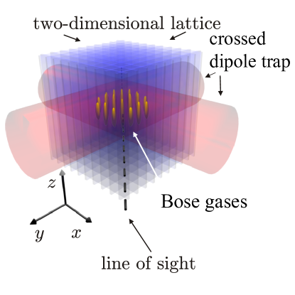
Figure 1: (Color online) Schematic of the experimental set-up. A BEC of ⁸⁷Rb atoms was initially prepared in the crossed-dipole-harmonic trap. A 2D optical lattice along the $x$-$y$ direction was then adiabatically ramped on to create an array of quasi-1D tubes. The crossed dipole-trap was then turned off and the expansion dynamics in the presence of the 2D periodic potential were investigated by direct imaging. The line of sight was at 45 degrees from the lattice directions (45 degrees from $x$ and $y$). The 2D atom density distribution was recorded after various expansion times.

In previous work Reinhard et al. (2013), we reported a similar yet richer situation in which the expansion dynamics took place in an array of quasi-1D tubes created by a 2D lattice. Atoms expanded along the tubes as they underwent their transverse dynamics. This made it possible to observe a self-trapping transition “on the fly”, as the overall density steadily dropped due to the axial expansion.

A BEC of $N\sim 3.5\times 10^{5}$ ${}^{87}\text{Rb}$ atoms was initially prepared in a crossed-dipole-harmonic trap with transverse frequency $\omega_{\perp}=2\pi\times 38$ Hz and vertical confinement $\omega_{||}=2\pi\times 94$ Hz. It was then loaded into a 2D square-lattice potential with lattice spacing $d=385$ nm. The experimental set-up is shown in Fig. 1. The blue-detuned 2D lattice was ramped up in time according to $I(t)\propto[1-(t/\tau)]^{-2}$, reaching a final lattice depth of $V_{o}=7.25E_{R},9.25E_{R},11E_{R}\ \text{or}\ 13E_{R}$ and creating an array of 1D tubes. Here $I$ is the lattice intensity, $\tau=4.15$ms is the time constant and $E_{R}=h^{2}/(8Md^{2})$ is the recoil energy where $d$ is the lattice spacing. After the initial preparation all the harmonic confining potentials were suddenly turned off so that the atoms could expand in the 2D lattice. The expansion dynamics were investigated by direct imaging. The line of sight was along a direction 45 degrees between the lattice directions (45 degrees from $x$ and $y$), and the image of the 2D density-distribution squared was recorded as a function of time. The main finding was a suppressed expansion rate of the RMS width of the density profile along the lattice, consistent with MQST. However, the expansion rate did not agree with the mean field predictions. Moreover, no signature of MQST behavior predicted by the mean-field theory was observed, such as the formation of steep edges or a hole at the center of the density profile.

III.1 Mean Field: Coupled GPEs

For the 2D lattice configuration, the total external potential was given by $V_{ext}(x,y)=V_{lat}(x,y)+V_{dip}(\vec{x})$ with $V_{lat}(x,y)=V_{o}[\sin^{2}(\pi x/d)+\sin^{2}(\pi y/d)]$ the lattice potential and $V_{dip}(\vec{x})=\frac{1}{2}M\omega_{\perp}^{2}(x^{2}+y^{2})+\frac{1}{2}M\omega_{||}^{2}z^{2}$ the confinement introduced by the crossed-dipole-trap. The dipole confinement was turned off during the expansion and therefore it was only relevant for determining the initial conditions. A small anti-trapping potential remained due to the Gaussian profile of the laser beams that generated the lattice. The parameters of the crossed dipole trap used to set up the initial state in the theoretical model were chosen so that the atom distribution matches the initial spatial extent and energy of the atoms in the experiment. The experimental parameters cannot simply be used because atoms in the experiment do not expand by as much as mean field theory predicts when the blue-detuned lattice is turned on. The explanation for this may be related to the anomalous self-trapping that is the subject of this paper, but a full understanding of that effect will require future work. The suppressed atom expansion during the turn-on of the lattice might also mean that the initial atom correlations are not the same as in the mean field model.

Assuming that only the lowest band of the 2D optical lattices was populated, a condition that was satisfied in the experiment, we write $\Psi$ in terms of the lowest band Wannier orbitals,

$$\Psi=\sum_{m,n}W(x-dn)W(y-dm)\Phi_{nm}(z,t),$$ (9)

where $\Phi_{nm}$ is the order parameter describing the tube centered at lattice site $(n,m)$, and $N_{nm}(t)=\int dz|\Phi_{nm}(z,t)|^{2}$ is its corresponding atom number. The normalization condition $\sum_{n,m}N_{nm}=N$ with $N$ the total number of atoms is satisfied.

By assuming $\Phi_{nm}(z,t)=\psi_{nm}(t)\phi_{nm}[z,N_{nm}(t)]$ ($\int dz\left|\phi_{nm}[z,N_{nm}(t)]\right|^{2}=1$ and $N_{nm}=|\psi_{nm}(t)|^{2}$) and using a similar variational-method to the one described in Appendix A, we can obtain the following effective Hamiltonian,

$$H_{eff} = N\left[-4J+\frac{9}{25}U_{eff}\left(\frac{2}{\pi r^{2}}\right)^{2/3}N^{2/3}\right]$$ (10)

$$= N\left[-4J+\frac{9}{25}U\rho d^{3}\right]$$

where $r$ is the width of the wave packet in the lattice directions (in the lattice units). Here we have defined the 2D interaction strength as $U=\frac{g}{d}\int dxdy\ W^{4}(x)W^{4}(y)$. $U_{eff}=\left(\frac{9M\omega_{z}^{2}d^{2}U^{2}}{32}\right)^{1/3}$ plays a similar role as $U_{\alpha}$ in Appendix A, and $J=\int dx\ W(x-d)\left[\frac{\hbar^{2}}{2M}\frac{\partial^{2}}{\partial x^{2}}-V_{lat}\right]W(x)$. $\rho=\frac{3}{4d^{3}}\left(\frac{2N}{r^{2}\pi}\right)^{2/3}\left(\frac{2M\omega_{z}^{2}d^{2}}{3U}\right)^{1/3}$ is the 3D density at the center of the cloud. Based on the variational method, we predict that the MQST in the 2D optical lattice should take place when $U\rho d^{3}/J\geq\frac{100}{9}$.

Although the variational method roughly describes the global dynamics and gives the threshold value $\rho_{c}$ of the MQST, it only explicitly accounts for the expansion dynamics across the lattice but not along the tube’s direction. We first tried to adapt the variational methods to capture the expansion in both directions. For that purpose, we assumed the density profile along each tube $\phi_{nm}(z)$ to have either a Thomas-Fermi (TF) or a Gaussian shape with a width $R_{nm}(t)$ and a phase $\delta_{nm}(t)$. In the lattice direction on the other hand, the evolution of the amplitudes $\psi_{nm}(t)$ at each lattice site was numerically computed. Unfortunately, we found that it was quantitatively accurate only at very short times. The reason is that (in the experiment) atoms in the tubes rapidly expanded vertically with a number-dependent expansion rate. Since the atoms tunneled between neighboring tubes at the same time, these two processes destroyed the assumed Gaussian or TF shape in each tube and the ansatz broke down.

Since the variational method failed, we instead numerically solve for the axial dynamics. We neglect any temporal dependence of the Wannier functions, which is justified because the inter-well number/phase dynamics is much faster than the time associated with the change in shape of such functions. Generically, the wave-field $\Psi(\vec{x},t)$ can still be written in terms of Eqn. (9), so we keep $\Phi_{nm}(z,t)$ as an arbitrary function. After integrating out the lattice directions, we obtain the following Nonlinear Schrödinger Equations and solve them numerically.

$$i\hbar\dot{\Phi}_{nm}(z,t) =\left(-\frac{\hbar^{2}}{2M}\frac{\partial^{2}}{\partial z^{2}}+V_{dip}(dn,dm,z)+Ud|\Phi_{nm}(z,t)|^{2}\right)\Phi_{nm}(z,t)-J\left[\Phi_{n\pm 1,m}(z,t)+\Phi_{n,m\pm 1}(z,t)\right].$$ (11)

To characterize the MQST, we numerically compute the root mean square (RMS) transverse width, $x_{rms}$, of a vertical slice of the cloud centered at z=0 and with a width corresponding to $\pm 10\%$ of the total axial width (characterized by the Thomas-Fermi radius, $R_{z}$). The reason for selecting a slice instead of integrating over the whole cloud is to consider a sample of approximately constant density. Theoretically $x_{rms}$ is directly calculated as: $x_{rms}=\sum_{m}\rho_{m}m^{2}/\sum_{m}\rho_{m}$ where $\rho_{m}=\int_{-Rz/10}^{Rz/10}dz\sum_{n}|\Phi_{nm}(z,t)|^{2}$.

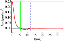
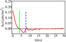
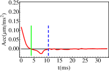
Figure 2: (Color online) The acceleration of $x_{rms}$ ($\ddot{x}_{rms}$) obtained from the mean field calculations for all lattice depths used in the experiment: (a) 7.25$E_{R}$, (b) 9.25$E_{R}$, (c) 11$E_{R}$ and (d) 13$E_{R}$. From the sign of $\ddot{x}_{rms}$, the evolution can be separated into three different regimes indicated by green solid lines and blue dashed lines. The three regimes are discussed in detail in the text. MQST is signaled in the $x_{rms}$ as a negative acceleration. It starts at the green solid line and stops at $\sim t_{c}$ (indicated by the blue dashed line) when the acceleration-curves cross 0 from below. The values of $U\rho(t_{c})/Ja^{3}$ for the four depths in consideration at $t_{c}$ are $\{0.4,3.0,3.0,3.0\}$. Those correspond to $\rho(t_{c})/J=\{60,350,320,300\}$ $\mu\rm{m}^{-3}$$E_{R}^{-1}$ respectively.

The expansion along the tubes makes MQST a time-dependent phenomenon, since as the atoms freely expand, the density decreases with time until the system becomes too dilute to sustain self-trapping. To determine the critical value of $\rho/J$ at which MQST stops, we numerically calculate $\ddot{x}_{rms}$. We construct an approximation function that interpolates the numerical values of $x_{rms}(t_{i})$ at recorded time $t_{i}$. As shown in Fig. 2, the curves of $\ddot{x}_{rms}$ are not completely smooth, especially at long times, due to accumulated numerical errors. We define the critical time $t_{c}$ to be the time when the acceleration first crosses zero from below, i.e., it is negative for times shorter than the critical time due to the MQST (See Fig. 2). Note that $t_{c}$ as well as $\rho(t_{c})/J$ are only roughly estimated.

The variational method gives the criterion, $U\rho(t_{c})/Jd^{3}\approx 11$. Numerically, we found $U\rho(t_{c})/Jd^{3}=\{0.4,3.0,3.0,3.0\}$ for lattice depths $7.25$, $9.25$, $11$ and $13E_{R}$, which correspond to $\rho(t_{c})/J=\{60,360,320,300\}\ \mu\rm{m}^{-3}$ $E_{R}^{-1}$ respectively. Although the numerical values of $\rho(t_{c})/J$ are smaller than the value predicted by the variational method, they are almost constant, except for the one associated to the $7.25E_{R}$ curve, consistent with the general concept of a self-trapping threshold.

There are three distinct regimes clearly observed in $\ddot{x}_{rms}$ which we use to characterize the dynamics. We will discuss those different regimes in detail below.

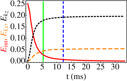
Figure 3: (Color online) Time evolutions of: the kinetic energy along the lattice direction ($E_{kx}$, orange dashed line), the kinetic energy along $z$ ($E_{kz}$, black dotted line), and the interaction energy ($E_{int}$, red solid line). This plot is computed using the mean field model for a $7.25E_{R}$ lattice. The vertical lines are at the same positions as in Fig. 2 (a).

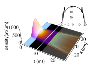
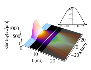
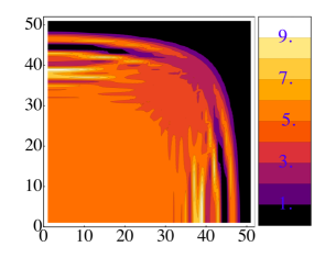
Figure 4: (Color online) Expansion dynamics predicted by the mean field calculations for the lowest lattice depth (7.25 $E_{R}$): Panel (a) displays the evolution of the density profiles at $z=0$, after integrating along one transverse direction, $\tilde{N}(x,t)$. Panel (b) displays the same density profiles, but after integrating along a direction that is 45 degrees between the $x$ and $y$ axes (as done in the experiment). Panel (c) shows transverse density-profiles at $z=0$, $\tilde{N}(x,y)$, during the MQST regime at $t=8.7\text{ms}$. The insets in Panel (a) and (b) are intersecting profiles at $t=8.7\text{ms}$ marked by white lines in the 3D density plots.

III.2 General Behavior: Three Different Regimes

Based on the sign of $\ddot{x}_{rms}$, we classify the dynamical evolution of the system into three different regimes: Initial expansion (Exp), MQST, and Ballistic expansion (BE). Each regime has a distinct behavior which can be further characterized by other observables such as the ratio between interaction and kinetic-energies (Fig. 3) and the shape of the density profile (See Fig. 4).

$\bullet$ Initial expansion (Exp):

The initial expansion regime describes early-times during which the atoms at the center of the cloud expand transversely. We determine this regime by looking at the time period over which the transverse RMS-width of the cloud expands with a non-linear rate (positive acceleration, $\ddot{x}_{rms}>0$). During this time the density-profile remains smooth. The interaction energy decreases very rapidly and is converted into kinetic energy along the axial and transverse directions. In contrast to a non-interacting system, in which the initial potential energy in the trap is converted to kinetic energy while the width of the quasi-momentum distribution stays constant, the mean field interactions cause a broadening of the quasi-momentum distribution whose width grows until it reaches values of quasi-momenta at which the effective mass becomes negative. At this point, sharp peaks in the density profile develop.

For the $7.25E_{R}$ lattice, the initial-expansion takes place within the first 5ms [See Fig. 2 (a)] after having turned off the parabolic-confinement. In Fig. 4 (a) and  4 (b), we also show the time evolution of a horizontal slice of the cloud $z=0$, after having integrated along one transverse direction (along $x$), and a direction 45 degrees from the transverse direction (45 degrees from $x$ and $y$), which is the line of sight direction in the experiment.

$\bullet$ Macroscopic Quantum Self-Trapping (MQST): At intermediate times ($t\sim 5-12$ms for the lowest lattice depth) MQST is signaled by the RMS-width of the cloud. During the MQST regime the interaction energy decreases slowly and remains comparable to the kinetic energy of the atoms in the lattice. The interplay between interatomic interactions and the atomic-density-gradient at the cloud edges prevents atoms from tunneling outward. In this regime the atoms start to pile up at the edges, and a hole forms at the center of the cloud [see Fig. 4 (c)]. The radial expansion slows-down or even stops as illustrated by a negative $x_{rms}$ acceleration. The slowing-down can also be linked to the population of a large number of quasi-momentum states with negative effective-mass.

Global observables, such as the RMS-width are easily measured and characterized. They encode some important signatures of MQST. However, MQST is an inherently local effect, and important information can be hidden in the global probes. For example, although the formation of steep edges and a hole is shared by the MQST phenomena in both 1D and 2D lattices and is observable in the RMS-width, there are more features in the 2D system.

In the MQST regime, the atom distribution in the lattice is no longer smooth, and its profile evolves from having a circular shape to a square one. Atoms at $45^{o}$ to the lattice axes are only self-trapped at larger radii, since the corresponding density gradients are smaller than in the lattice directions. This gives rise to the square fort-like barrier around the edges, seen in Fig. 5. The formation of steep edges also happens in the 1D system, but in 2D there is always a direction along which atoms can tunnel. Since they are not fully frozen, the self-trapped edges are not stationary as in the 1D case, but instead they evolve with time.

The shape of the integrated density-distribution strongly depends on the direction along which the integration is performed (See Fig. 4(a) and Fig. 4 (b)). For example, while the peaks at the edges, signaling the hole at the center of the cloud, are clearly visible in Fig. 4 (a), when the imaging direction is along the lattices, they are barely visible when the imaging direction is along the diagonals as in Fig. 4 (b).

$\bullet$ Ballistic Expansion Regime (BE): Because atoms expand axially along the tubes, the interatomic interactions decrease as time evolves and at some point they are no longer strong enough to enforce the self-trapping mechanism. This determines the interruption of the MQST and the onset of the ballistic regime. In this regime mean-field interactions have decreased so significantly that an analysis in terms of single-particle eigenstates and eigenmodes can be carried out.

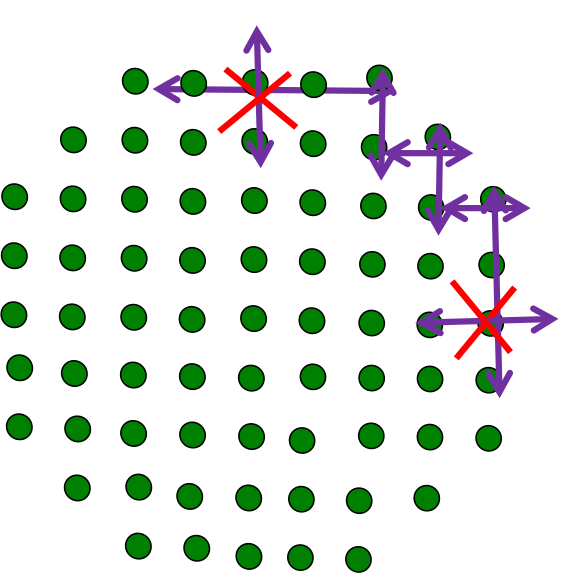
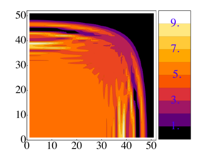
Figure 5: (Color online) Panel (a) is a schematic picture of the tunneling in 2D optical lattices. In 2D, no site is self-trapped in all directions so atoms are not fully frozen. The arrows show the directions that atoms may tunnel while the crosses mean that tunneling along those directions is forbidden by MQST. Panel (b) is a density contour plot of a square fort-like barrier developed during the MQST regime.

III.3 Comparison with the experiment

The experimentally measured RMS-widths are slightly different from the $x_{rms}$ defined above. In the experiment the density-square distribution, instead of the density, was directly measured. To mimic the RMS-widths measured in the experiment, we define another RMS-width, denoted as $\sigma_{n^{2}}$. To get $\sigma_{n^{2}}$, we square the 1D distribution $\rho_{m}$ ($\rho_{m}$ is obtained by integrating the 3D density distribution along a line 45 degrees from a lattice direction over a slice centered at $z=0$) and convolve it with a Gaussian of RMS-width $1.7\mu\rm{m}$ (the imaging system resolution) to get the convolved-density-square-distribution $n^{2}_{m}$ or $\tilde{\rho}_{m}$. The convolution procedure mimics the finite-size-resolution of the imaging system. Finally, $\sigma_{n^{2}}$ is directly calculated by the definition: $\sigma_{n^{2}}=\sum_{m}\tilde{\rho}_{m}m^{2}/\sum_{m}\tilde{\rho}_{m}$. This process removes fine features from the theoretical curves that are not resolvable in the experiment.

Another observable measured in the experiment was the Thomas-Fermi radius $R_{z}$ of the atomic density along $z$. It was obtained by fitting the atomic density distribution, after integrating along the transverse directions, to $\frac{3}{4R_{z}}\max[0,1-(z/R_{z})^{2}]$. Because the initial width of the cloud is sensitive to the loading procedure and because the mean field treatment tends to overestimate the initial width of the cloud compared to the one measured in the experiment, we use different initial sizes to compare with the experiment, subject to the constraint of matching axial expansion rates at long times. The latter just ensures that we are using the correct total energy, which is conserved during the evolution. Comparisons between the numerical simulations and the experimental data are shown in Figs. 6 and 7. In general, the theory overestimates the expansion rate of the RMS-widths. Only for $7.25E_{R}$ does the mean-field theory roughly capture the experimental observations at short times. For deeper lattice depths, such as $13E_{R}$, the mean-field theory fails to reproduce the observed dynamics.

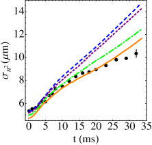
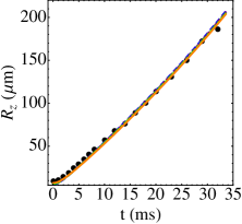
Figure 6: (Color online) The evolution of (a) $\sigma_{n^{2}}$ and (b) $R_{z}$ for $7.25E_{R}$ from mean field calculations and the experiment. Each black point is the average of 10 experimental measurements. In Panel (a), the error bars represent random uncertainty, but an overall systematic uncertainty of $0.5\mu$m associated with the imaging resolution is not included. To illustrate the dependence of the mean-field dynamics on the initial width, we show the evolution of $\sigma_{n}^{2}$ for different initial conditions for the $7.25E_{R}$ lattice. Each line corresponds to a particular initial condition, subject to the constraint of matching axial expansion rates at long times. In Panel (b), error bars are not shown, since we are mainly interested in the long time dynamics when $R_{z}$ is very large and the error bars are negligible. Even with different initial conditions, the expansion rates along $z$ are almost the same, therefore in Panel (b) all lines are almost on top of each other.

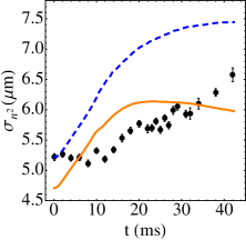
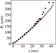
Figure 7: (Color online) Time evolution of (a) $\sigma_{n^{2}}$ and (b) $R_{z}$ for $13E_{R}$ from mean field calculations and the experiment. As in Fig. 6, the solid and dashed lines are simulation results and each corresponds to a particular initial condition. The long-time dynamics of $\sigma_{n^{2}}$ is sensitive to the initial width of the cloud also at $13E_{R}$. The black points are experimental data.

The long-time dynamics of $\sigma_{n^{2}}$ predicted by the mean field method is sensitive to the initial width of the cloud. When the initial RMS-width is larger, the MQST boundary is further away from the center and thus it takes more time for the RMS-width to reflect the presence of MQST at the edges. In contrast, the MQST is more visible for smaller initial RMS-widths, as shown in Figs. 6 and 7.

The plots in Fig. 4 share the same initial condition as the dashed blue line in Fig. 6. With this initial condition, the MQST effect is weak and the self-trapping signatures, such as peaks at the edges [Fig. 4  (a)] and a hole in the middle [Fig. 4 (c)], are not very pronounced. These self-trapping signatures were not seen in the experiment even when imaged from above. These characteristic signatures might be visible in future experiments with smaller lattice depths, smaller initial RMS-widths and larger values of $R_{z}$.

IV Beyond Mean-Field Model

As shown in Sec. III, the mean-field treatment does not correctly describe the experiment. A fundamental limitation of this treatment is that it assumes all the atoms are in the condensate and neglects condensate depletion due to quantum correlations or thermal fluctuations (coming from an initial thermal component or non-adiabatic effects as the lattice is turned on). Condensate depletion modifies the dynamics predicted by the single mode approximation. In an attempt to include quantum fluctuations, we use an approximate TWA Polkovnikov (2010); Blakie et al. (2008); A.Sinatra et al. (2002). The TWA incorporates leading order corrections to the dynamics expanded around the classical (GPE) limit. The whole idea of the TWA is that the expectation value of a quantity at time $t$ can be determined by solving the classical equations of motion from 0 to $t$ and sampling over the Wigner distribution at time $t=0$. The TWA is guaranteed to be accurate at short times. For longer times, there are also higher order corrections to the classical trajectories. In a 3D lattice (0D condensate in each well) there are two limiting regimes where the Wigner function can be easily found and has been shown to capture the exact dynamics well Polkovnikov (2010). One is the very weakly interacting regime in which the system is almost an eigenstate of the noninteracting Hamiltonian, a product of coherent states. The other case is the strongly interacting regime with commensurate filling, in which the system is a Mott insulator. In this case the many body wave function is mostly a product Fock state $\prod_{j=1}^{L}|n\rangle_{i}$ with $n$ the filling factor. The semiclassical wave function is $\prod_{j=1}^{L}\sqrt{n}\exp{({\rm i}\phi_{j})}$ and the corresponding Wigner function is characterized by independent random variables $\phi_{j}$ uniformly distributed between $(0,2\pi)$.

The case that we are dealing with now has the complication that not only is it in the intermediate regime where neither of the two limiting cases holds, but also, instead of a 0D condensate within a lattice site we have a quasi-1D gas. Finding the Wigner function therefore is not a trivial task. Prior work done for two coupled 1D tubes Hipolito and Polkovnikov (2010) has already shown the importance of taking into account quantum correlations for the proper characterization of the dynamics. Consequently, we expect that beyond-mean-field corrections will play an important role in our system.

With this goal in mind and subject to the limitation that the pure mean field dynamics involve the propagation of thousands of coupled GPEs, we implement the TWA in an ad-hoc way which we refer to as aTWA. We account for initial phase fluctuations within each tube by adding random phase factors: $\phi_{nm}(t=0)\rightarrow\eta\cdot\theta_{nm}$, where $\theta_{nm}$ is a uniformly distributed random variable between $0$ and $2\pi$, and $\eta$ parameterizes the strength of the phase fluctuations. When $\eta=0$, the initial conditions correspond to a fully coherent array of 1D gases and when $\eta=1$, we have an initially fully incoherent array. $0<\eta<1$ corresponds to a partially coherent array. Since $\eta$ is not determined in the theory, we compare the results for different $\eta$ to experiment, and choose the most similar one. We average the results over at least $20$ initial configurations.

Besides phase fluctuations, we also study the effect of including number fluctuations in the initial conditions. The results obtained using the aTWA are described in detail in the following subsections.

The aTWA considerably improves the agreement between theory and experiment. The value of $\eta$ that optimizes the agreement with the experiment increases with increasing lattice depth. This is expected, since as tunneling between tubes becomes weaker, phase coherence is suppressed. The noise introduced by those random phases quickly generates local self-trapping everywhere, suppressing the transverse dynamics until, due to the axial expansion, interactions drop so significantly that the system goes to the ballistic expansion regime. Noise also tends to suppress the hole formation. See Fig. 8.

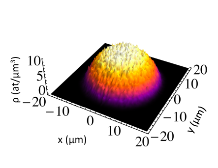
Figure 8: (Color online) Transverse density profiles at $z=0$ during the MQST regime at $t=8.7\text{ms}$ for the $13E_{R}$ lattice obtained from the aTWA results.

IV.1 Comparison between theory and experiment: phase fluctuations

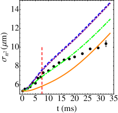
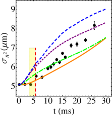
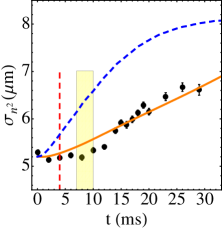
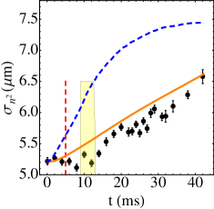
Figure 9: (Color online) Mean-field, aTWA and experimental results for the evolution of $\sigma_{n}^{2}$ for all lattice depths used in the experiment. The lattice depths are (a) 7.25$E_{R}$, (b) 9.25$E_{R}$, (c) 11$E_{R}$ and (d) 13$E_{R}$. At low lattice depth, a small $\eta$ seems to account for the observed behavior at short times. The dashed blue line is the result of a mean-field calculation of the dynamics with no random phase between the tubes ($\eta=0$). The dotted purple line is for $\eta=0.2$, the dashed-dotted green lines are for (a) $\eta=0.4$ and (b) $\eta=0.5$, and the solid orange line is for $\eta=1$. The dashed vertical red lines indicate the transition from MQST to BE predicted by the aTWA. The yellow shadow regions indicate the $t_{c}$ inferred from the experimental data.

Phase fluctuation among tubes substantially suppresses the expansion dynamics. To illustrate this effect, consider the toy model of a double-well with initial relative phase difference $\phi(0)$. The critical value of $\Lambda$ ($\Lambda$ is proportional to the ratio of the on-site interaction energy and the tunneling matrix element between two wells) which determines the MQST-to-diffusive transition depends on $\phi$ as,

$$\Lambda_{c}=2\left(\frac{\sqrt{1-z(0)^{2}}\cos[\phi(0)]+1}{z(0)^{2}}\right),$$ (12)

where $z$ is the fractional population difference between the two wells, $z=\frac{N_{L}-N_{R}}{N_{L}+N_{R}}$. In this case one can see that even when the initial population imbalance is small, $z(0)\ll 1$, the system can become self-trapped if $\phi(0)\to\pi$ ($\Lambda_{c}\rightarrow 1$). In other words the critical value of $\Lambda_{c}$ decreases with increasing $\phi(0)$.

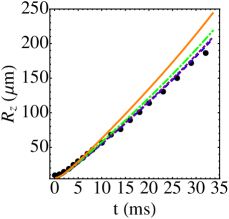
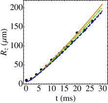
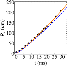
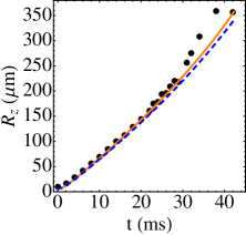
Figure 10: (Color online) Evolution of $R_{z}$ for all lattice depths used in the experiment. The dots show experimental data and the solid and dashed lines show the predictions obtained from the aTWA for different $\eta$. The lattice depths are (a) 7.25$E_{R}$, (b) 9.25$E_{R}$, (c) 11$E_{R}$ and (d) 13$E_{R}$. $R_{z}$ is obtained by fitting the density along $z$ to a Thomas-Fermi profile. The theoretical curves use the same parameters as the ones shown in Fig. 9.

Our simulation agrees with this expectation. Fig. 9-10 show the transverse RMS $\sigma_{n^{2}}$ and the vertical Thomas-Fermi radius $R_{z}$. The aTWA treatment agrees much better with experimental observations, especially for the deepest lattices. In Fig. 9, we can see that the greater the $\eta$ the slower is the expansion rate of $\sigma_{n^{2}}$. When $\eta=1$, i.e., when the phase fluctuations are maximal , the expansion rate of $\sigma_{n^{2}}$ reaches its smallest value.

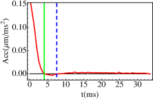
Figure 11: (Color online) $\ddot{x}_{rms}$ calculated using the aTWA for different lattice depths and for the corresponding optimal $\eta$, (a) $7.25E_{R},\eta=0.4$ and (b) $13E_{R},\eta=1$. The boundaries between MQST and BE are indicated by the blue dashed lines. In panel (a), the boundary between EXP and MQST is indicated by the green solid line. In panel (b), because $\ddot{x}_{rms}$ is almost 0 at all times, it can be interpreted as the self-trapping starts at $t=0$ ms.

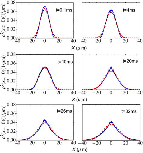
Figure 12: (Color online) Transverse density profiles: The solid/dashed lines are obtained from the aTWA results for the $V=7.25E_{R}$ lattice and for $\eta=0.4$. The profiles are taken at $z=0$ and viewed transversely at an angle $45^{o}$ from the lattice axis and normalized to $1$. The solid blue lines indicate the theoretical profiles before convolution and the dashed black lines after convolution. The red solid points are averaged experimental data of 10 measurements.

Although the modeled curves with the appropriate $\eta$ are never too far from the data, for $V_{0}\geq 11E_{R}$, the experiment shows a more delayed and more sudden onset of ballistic expansion than the model. For $V_{0}=7.25E_{R}$, $\eta\approx 0.4$ best fits the early evolution, when there is MQST. For larger $V_{0}$, $\eta=1$ clearly fits best for the short evolution time. For $V_{0}=7.25E_{R}$, $\eta\approx 0.4$, the three regimes predicted by the pure mean field model are still visible, although $\ddot{x}_{rms}$ becomes barely negative in the MQST regime. On the other hand, for the deeper lattices, the random initial phases cause a fast development of site-to-site density fluctuations and the formation of localized domains randomly distributed throughout the tube array. In contrast to the pure mean field model, localization occurs without the formation of sharp edges, there is no reflection from them and $\ddot{x}_{rms}$ never becomes negative. Instead, it asymptotically approaches zero from above as shown in Fig. 11. MQST always disappears when the density drops below a critical value that depends on $V_{0}$. The model predicts the following values for the transition to a ballistic regime, $\rho(t_{c})/J=\{840,1900,1970\}\mu{\rm m}^{-3}E_{R}^{-1}$ for $V_{0}/E_{R}=\{9.25,11,13\}$. We can compare these values with the ones measured in the experiment which occur when the ratio $\rho(t_{c})/J=\{1190\pm 310,860\pm 190,910\pm 210\}\mu{\rm m}^{-3}E_{R}^{-1}$ for $V_{0}/E_{R}=\{9.25,11,13\}$ respectively. We can see that the ratio of $\rho(t_{c})/J$ in the experiment is roughly constant. However, while the values of $\rho(t_{c})/J$ predicted by the aTWA are almost the same for $11E_{R}$ and $13E_{R}$, $\rho(t_{c})/J$ for $9.25E_{R}$ is only half of that value. On the other hand, the actual $\rho(t_{c})/J$ value predicted by the aTWA at $9.25E_{R}$ is closer to the observed value.

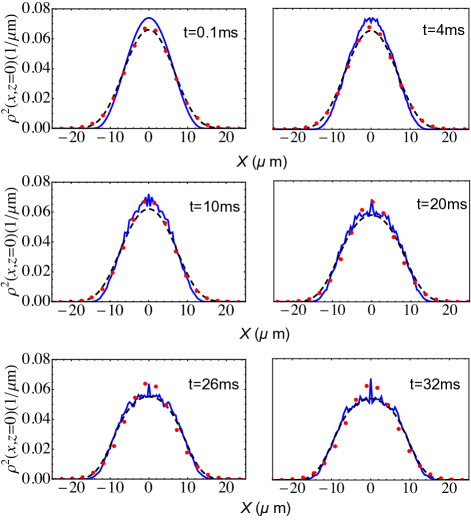
Figure 13: (Color online) Transverse density profiles: The solid/dashed lines are obtained from the aTWA results for the $V=13E_{R}$ lattice and for $\eta=1$. The profiles are taken at $z=0$ and viewed transversely at an angle $45^{o}$ from the lattice axis and normalized to $1$. The solid blue lines indicate the theoretical profiles before convolution and the dashed black lines after convolution. The red points are averaged experimental data of 10 measurements.

Figures 12-13 show the density profiles measured experimentally for the shallowest and deepest lattices and the corresponding theoretically computed profiles. For the $7.25E_{R}$ lattice, one can see a good agreement after the theory curves are convolved to account for the imaging system resolution. However, the theoretical distributions are not well fitted by a Gaussian at longer times. The experimental distributions on the other hand always retain a Gaussian profile. In general phase fluctuations prevent the hole formation and help to keep the density distributions closer to a Gaussian profile.

IV.2 Number Fluctuations

So far we have included only phase fluctuations. However, we know that in the superfluid regime relative atom number fluctuations provide the dominant beyond-mean-field corrections. To investigate the role of number fluctuations in the expansion dynamics, we introduce number fluctuations in the initial conditions. We implement this by allowing $\approx 1/\sqrt{N_{nm}}$ fluctuations in the atom number in each tube, with $N_{nm}(0)$ the total number of atoms in a tube centered at $\vec{n}=\{n,m\}$. We focus on the case $V_{0}=7.25E_{R}$. The results are shown in Fig.  14, where we can see that number fluctuations do suppress the expansion rate of the cloud but by only a small amount.

Figure 14: (Color online) Time evolution of $\sigma_{n^{2}}$ computed for a $7.25E_{R}$ lattice and for $\eta=0$. The red dashed line shows the result when number fluctuations are neglected, and the blue solid line shows the result when number fluctuations ($\approx 1/\sqrt{N_{mn}}$) are included. The plot clearly shows that number fluctuations suppress the expansion, but only by a small amount.

IV.3 Phase And Number Fluctuations

In the intermediate regime – between the superfluid and Mott phases – both quantum and number fluctuations are relevant but constrained by the corresponding Heisenberg uncertainty relation. To get an upper bound of the amount of localization predicted by the aTWA, we add both number fluctuations ($\approx 1/\sqrt{N_{nm}}$) and phase fluctuations in the initial conditions. The results are shown in Fig.  15. Indeed the addition of both phase and number fluctuations helps to suppress the expansion rate of the cloud for moderate $\eta$ (as the $7.25E_{R}$ case) but for large $\eta=1$ the addition of number fluctuations is barely noticeable. In other words, the curves with number and phase fluctuations are quite similar to the curves with phase fluctuations only.

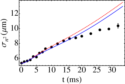
Figure 15: (Color online) aTWA results for the time evolution of $\sigma_{n^{2}}$ for a 7.25$E_{R}$ lattice and for $\eta=0.35$. The red dashed line shows the result when only phase fluctuations are included, and the blue solid line shows the result when both number fluctuations ($\approx 1/\sqrt{N_{mn}}$) and phase fluctuations are included. The plot shows that number fluctuations slightly suppress the initial expansion rate.

In summary, so far we have accounted for the quantum correlations developed in the tubes by adding an overall random phase in a phenomenological way. Although this procedure pushes the theory closer to the experimental observations, a fundamental problem with the aTWA is that it misses the correlations within each tube. Those might be the key ingredient responsible for the observed localization at short times due to the additional energy cost they impose when atoms tunnel from one tube to the next. Those correlations are expected to play a major role at short times when interactions are dominant. A significantly better treatment could be obtained by computing the full Wigner function of the interacting systems. The latter could, in principle, be achieved by starting with the Wigner function of the non-interacting system (which is known) and then by adiabatically increasing the interactions to the desired value. The large number of degrees of freedom in consideration substantially complicates this implementation.

V Beyond The aTWA—Two Coupled Tubes

In order to test the validity of the various approximations used so far, we now turn to a simplified model system which is amenable to a numerically exact treatment using the t-DMRG. In the following we will consider a configuration of two coupled tubes (see Fig. 16) and compare the dynamics of this minimal system to the one obtained with the pure GPE and the aTWA methods. To be more specific, we replace in our toy two-tube model the axial parabolic trapping potential along the tubes by a box potential which is easier to treat numerically, and we create the population imbalance at the beginning of the dynamics by choosing different chemical potentials on the two tubes, which we then set to zero instantaneously in order to mimic the time evolution in the experiment. Note that when removing the box potential in this setup, the dynamics at the edges of the cloud can dominate the tunneling between the two tubes. Therefore, we find it more convenient to keep the box turned on throughout the time evolution. Moreover, in order to avoid the complications of dealing with a continuum system, we assume that along each tube there is a weak lattice (with $L$ lattice sites) and use the tight-binding approximation to describe the dynamics. This gives rise to a Bose-Hubbard model,

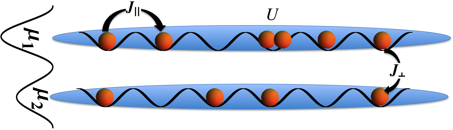
Figure 16: (Color online) Schematic configuration of the two-tube system.

$$H= -J_{\|}\sum_{l=1,2}\sum_{<i,j>}\left(\hat{a}_{l,i}^{\dagger}\hat{a}_{l,j}+h.c\right)+\sum_{l,i}\frac{U}{2}\hat{n}_{l,i}(\hat{n}_{l,i}-1)$$ (13)

$$-J_{\perp}\sum_{i}\left(\hat{a}_{1,i}^{\dagger}\hat{a}_{2,i}+h.c\right)-\sum_{l,i}\mu_{l}\hat{n}_{l,i},$$

where $J_{\|}$ is the tunneling matrix element between nearest neighboring sites within each tube, $J_{\perp}$ is the tunneling matrix element between tubes, $U$ is the on-site interaction strength and $\mu_{l}$ is the chemical potential on tube $l$ ($l=1,2$). The difference in chemical potentials $\mu_{1}-\mu_{2}$ equals the bias between the two tubes which is adjusted in order to obtain the desired population on each of the tubes. Note that we assume tunneling between the tubes takes place at nearest neighbouring sites only, so that we obtain a ladder geometry.

V.1 The DMRG Method

DMRG is a numerical method which is capable of obtaining ground-state properties of (quasi)one-dimensional systems with very high efficiency and accuracy for lattices with up to several thousand sites. This is achieved by working in a truncated basis of eigenstates of reduced density matrices obtained for different bipartitions of the lattice. The so-called discarded weight, which is the sum of the weights of the density-matrix eigenstates that are neglected and which should be as small as possible Schollwöck (2005) quantifies the error of the method. Also, its time-dependent extensions (t-DMRG) can treat the real-time evolution of strongly correlated quantum many-body systems substantially larger than the ones amenable to exactly diagonalizing the Hamiltonian and with an accuracy which can be, at short and intermediate times, similar to what is achieved in ground-state calculations. Here, we use this accuracy to obtain high precision numerical results. During the evolution, we aim for a discarded weight of $<10^{-9}$ and keep up to $500$ density-matrix eigenstates for systems with $L=40$ sites in each tube. We apply a time step of $\Delta t=0.01/J_{\|}$ and find a discarded weight of $\lesssim 10^{-6}$ at the end of the time evolution displayed in the plots.

1D Bose gases are typically characterized by the dimensionless parameter $\gamma$ Dunjko et al. (2001), the ratio of the mean field interaction energy per particle calculated without correlations to the kinetic energy calculated with maximal correlations. A weakly interacting 1D gas ($\gamma\ll 1$) is well described by mean-field theory. In contrast, in the strongly interacting regime, $\gamma\gg 1$, atoms avoid each other to reduce mean field energy and the bosons behave like noninteracting fermions Girardeau (1960). In the 1D Bose-Hubbard model $\gamma\approx\frac{U}{J}$.

In our ladder configuration we will use $\gamma=\frac{U}{J_{\|}}$ to quantify the interaction strength of the system. This is expected to be a good characterization when the intertube tunneling is much smaller than the intratube tunneling ($J_{\perp}\ll J_{\|}$). We set $J_{\|}=1$ in all cases and vary both $\gamma$ (by changing $U$) and the density. Table 1 summarizes the set of parameters that we use to study the dynamics. $N_{total}$ is the total particle number in the system.

	UN${}_{\text{total}}$	J∥	J⟂	$L$ ( lattice sites)
case 1	30	1	0.025	40
case 2	30	1	0.05	40
case 3	30	1	0.1	40
case 4	60	1	0.05	40
	N${}_{\text{total}}$	J∥	J⟂	$L$ ( lattice sites)
case 5	30	1	0.05	40

Table 1: Set of parameters and different initial conditions used to study the dynamics. $N_{total}$ is the total particle number in the ladder. $U$ is the on-site interaction strength, $J_{\|}$ is the nearest neighbor tunneling matrix element within each tube, and $J_{\perp}$ is the tunneling matrix element between tubes.

V.2 Short-Time Dynamics

Even in this simpler two-tube system the many-body dynamics after a quench can be quite complicated. To compare the differences between results obtained using the mean-field theory, the aTWA and the t-DMRG, and to check the validity of the aTWA, we first focus on the short-time dynamics, for which we can obtain analytical expressions and numerical results.

A quantity that gives relevant information about the system’s dynamics is the total particle number in each tube, i.e., $N_{l}=\sum_{i}n_{l,i}$ with $n_{l,i}=\langle\hat{n}_{l,i}\rangle$. Heisenberg’s equations of motion for the atom number in the tubes then read ($\hbar\equiv 1$),

$$\frac{d}{dt}N_{l} = -iJ_{\perp}\sum_{i}\left(\langle\hat{a}_{l^{\prime},i}^{\dagger}\hat{a}_{l,i}\rangle-\langle\hat{a}_{l,i}^{\dagger}\hat{a}_{l^{\prime},i}\rangle\right),$$ (14)

$$\frac{d^{2}}{dt^{2}}N_{l} = -\frac{J_{\perp}U}{2}\sum_{i}\langle\left\{\hat{n}_{l,i}-\hat{n}_{l^{\prime},i},\hat{a}_{l^{\prime},i}^{\dagger}\hat{a}_{l,i}+\hat{a}_{l,i}^{\dagger}\hat{a}_{l^{\prime},i}\right\}\rangle$$ (15)

$$-2J_{\perp}^{2}(N_{l}-N_{l^{\prime}}),$$

where $l^{\prime}\neq l$ denotes the position in either tube 1 or 2.

Generally, for the ground state, $\text{Im}[\langle a_{l,i}^{\dagger}a_{l^{\prime},j}\rangle]=0$ (there are no currents in the system) and therefore the first derivative of $N_{l}$ is zero at $t=0$, i.e., $\frac{d}{dt}N_{l}\big{|}_{t=0}=0$.

The second derivative of $N_{l}$ is generally non-zero when there is a population imbalance between the two tubes, due to the second term on the right hand side of Eq. (15). The first term accounts for the role of interactions in the dynamics and involves four-particle correlation functions, which can play a fundamental role in the dynamics. For strongly repulsive bosons (hard-core bosons), on-site occupancies $>1$ are energetically forbidden, so the four-particle correlations vanish. Therefore only the term proportional to the population imbalance contributes to the dynamics. Hence, the dynamics of hard-core bosons are governed by,

$$\frac{d^{2}}{dt^{2}}N_{l}=-2J_{\perp}^{2}(N_{l}-N_{l^{\prime}}).$$ (16)

Analytical expressions for the short time dynamics can also be obtained using the mean-field (GPE) approximations and the aTWA.

At the mean-field (GPE) level, the operators $\hat{a}_{l,i}$ are replaced with c-numbers $\psi_{l,i}$. At $t=0$, the ground state corresponds to $\psi_{l,i}=\sqrt{n_{l,i}}e^{i\phi}$, and there is a global phase for all sites. Without loss of generality, $\psi_{l,i}(0)$ can be chosen as $\sqrt{n_{l,i}}$. Under the aTWA, $\psi_{l,i}$ is chosen as $\sqrt{n_{l,i}}$ times a global phase factor for each tube, i.e., $\psi_{l,i}(0)\rightarrow\sqrt{n_{l,i}}e^{i\theta_{l}\cdot\eta}$. As we explained in section IV, $\eta$ is a tunable parameter which characterizes the strength of phase fluctuations, and $\theta_{l}$ is a uniformly distributed random variable between $0$ and $2\pi$. The average can be computed analytically, and in the aTWA we obtain that the dynamics is governed by

$$\frac{d^{2}}{dt^{2}}N_{l}\bigg{|}_{t=0} = -2J_{\perp}^{2}(N_{l}-N_{l^{\prime}})$$ (17)

$$-2J_{\perp}U\frac{N_{l}-N_{l^{\prime}}}{L}\sqrt{N_{l}N_{l^{\prime}}}\frac{\sin^{2}(\pi\eta)}{\pi^{2}\eta^{2}}.$$

The second term in the above equation equals $-2J_{\perp}U\frac{(N_{l}-N_{l^{\prime}})}{L}\sqrt{N_{l}N_{l^{\prime}}}$ when $\eta=0$, and goes to $0$ when $\eta=1$, agreeing with the GPE and hard-core boson limits. Since $\frac{d}{dt}N_{l}\big{|}_{t=0}=0$, to lowest order, $N_{l}(t)=\frac{1}{2}\left(\frac{d^{2}}{dt^{2}}N_{l}\big{|}_{t=0}\right)t^{2}+N_{l}(0)$ at short times. Numerically, we can either directly calculate $\frac{d^{2}}{dt^{2}}N_{l}\big{|}_{t=0}$ from the initial wave-function at $t=0$ or extract it from $N_{l}(t)$ by fitting it to a quadratic polynomial. Here we use the second (fitting) method to get $\frac{d^{2}}{dt^{2}}N_{l}\big{|}_{t=0}$.

At $t=0$, Eq. (17) becomes,

$$\ddot{x}|_{t=0}=f(x)+g(x)\frac{\sin^{2}(\pi\eta)}{\pi^{2}\eta^{2}},$$ (18)

where $x=\frac{N_{1}}{N_{total}}$, $f(x)\equiv 2J_{\perp}^{2}(1-2x)$ and $g(x)\equiv 2J_{\perp}\frac{UN_{total}}{L}(1-2x)\sqrt{x(1-x)}$. When $x=0$, the population imbalance between the two tubes is maximum and all particles occupy the same tube. When $x=1/2$, atoms are equally distributed between the tubes.

The fitted values of $\eta$ that best reproduce the t-DMRG calculations obtained for different parameter regimes are shown in TABLE II. Fig. 17 shows comparisons between the aTWA results and the t-DMRG results for the optimal value of $\eta$ found for one of the parameters displayed in Table II. In the GPE limit ($\eta=0$), only the product $UN_{total}$ enters in the equations of motion, meaning that, as long as $UN_{total}$ is kept constant, the dynamics of the system are independent of $U$. This feature can be clearly seen in Eq. (17). This is certainly not the behavior predicted by the t-DMRG solutions which show a slow down of the dynamics with increasing $U$. The TWA is expected to fully capture the role of quantum correlations at short times. Interestingly, we find that $\ddot{x}|_{t=0}$ computed by t-DMRG is extremely well described by $f(x)+g(x)\frac{\sin^{2}(\pi\eta)}{\pi^{2}\eta^{2}}$ where $\eta$ is the only fitting parameter. The excellent agreement between t-DMRG and aTWA allows us to conclude that the aTWA captures well the quantum correlations parameterized by $\eta$ at short times in this simple two-tube model. We also see, that when $UN_{total}$ is fixed, in the parameter regime under consideration, the fitted values of $\eta$ that best reproduce the t-DMRG calculations are almost independent of the initial population imbalance, i.e., 1-2x, and the tunneling between tubes, i.e., $J_{\perp}$, when $J_{\perp}\ll J_{\|}$.

	$\eta$ for case 1	$\eta$ for case 2	$\eta$ for case 3	$\eta$ for case 4	$\eta$ for case 5
U=1	0.31	0.30	0.30	0.27	0.30
U=2	0.46	0.45	0.46	0.39	0.39
U=3	0.56	0.56	0.57	0.48	0.45
U=5	0.69	0.70	0.71	0.61	0.54

Table 2: Fitted values of $\eta$ for different set of parameters used to investigate the dynamics: at short times the t-DMRG dynamics is well captured by the aTWA when $\eta$ is used as a fitting parameter.

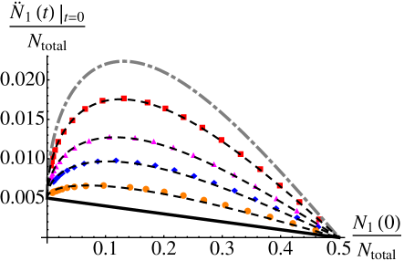
Figure 17: (Color online) $\frac{\ddot{N}_{1}}{N_{total}}|_{t=0}$ as a function of $\frac{N_{1}(t=0)}{N_{total}},J=0.05,UN_{total}=30$. The black solid line shows the GPE limit and the gray dash-dotted line the hard-core boson limit [see Eq. (18)]. The red squares, magenta upper-triangles, blue diamonds and orange disks show the initial curvature $\frac{\ddot{N}_{1}}{N_{total}}|_{t=0}$ extracted from the t-DMRG results at $U=1$, $U=2$, $U=3$ and $U=5$ respectively. The black dashed lines show the aTWA solutions using $\eta$ as a fitting parameter. The values of $\eta$ are listed in TABLE 2 . This plot is computed using the “case 2” parameters shown in Table II.

V.3 Long Time Dynamics

In Fig. 18 we compare the GPE, the aTWA and the t-DMRG dynamics. We see significant deviations between the approximate methods and the t-DMRG at longer times. This shows that the dynamics of the Bose-Hubbard model on this ladder geometry is dominated by correlation effects. Although at short times the t-DMRG results are well described by the aTWA results with an appropriate value of $\eta$, at longer times the aTWA fails to reproduce the many-body dynamics. This behavior confirms the relevance of quantum correlations neglected by the aTWA. Those deviations are consistent with the deviations we saw when trying to model the experimental data with the aTWA.

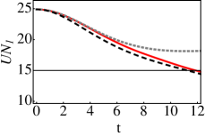
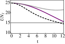
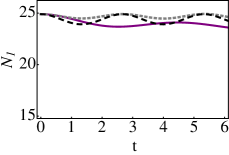
Figure 18: (Color online) Evolutions of $UN_{1}$ and $N_{1}$ as functions of time calculated using the DMRG and GPE methods. In panel (a) and (b), the values of $U$ are $1$ and $5$ respectively, while $UN_{total}$ is fixed to $30$. In panel (c) and (d), the values of $U$ are $2$ and $5$ respectively, while $N_{total}$ is fixed to $30$. In each panel, the solid line is the t-DMRG solution, the black dashed line is the mean-field calculation with no random phase (GPE). The dotted gray line is for (a) $\eta=0.3$, (b) $\eta=0.7$, (c) $\eta=0.4$ and (d) $\eta=0.53$.

Fig.18 shows that the weakly interacting regime is the regime where the GPE and the aTWA (with small $\eta$) predictions are closer to the t-DMRG results for longer time. The aTWA gives slightly better agreement at short times, indicating that for weak interactions it better captures correlation effects. In the strongly interacting regime, tunneling is greatly suppressed, especially in the presence of a large initial population imbalance. While in the GPE and the aTWA, $N_{1}(t)$ oscillates with more or less constant frequency and amplitude, in the t-DMRG, $N_{1}(t)$ oscillates with a lower frequency and gradually “relaxes” towards an equal distribution of atoms in the two tubes.

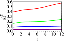
Figure 19: (Color online) $g_{l}^{(2)}$ as function of time in different regimes. The correlations are extracted from the t-DMRG results for the parameters describing case 2. Panel (a) shows $g_{1}^{(2)}$, $\frac{L}{N_{1}^{2}}\sum_{i}\langle\hat{n}_{1i}^{2}\rangle-n_{1i}$ and Panel (b) shows $g_{2}^{(2)}$, $\frac{L}{N_{2}^{2}}\sum_{i}\langle\hat{n}_{2i}^{2}\rangle-n_{2i}$. In each panel, from top to bottom, the lines correspond to $U=1$, $U=2$, $U=3$ and $U=5$ respectively.

To further quantify the quantum correlations (which are not captured in the GPE and are only partially captured in the aTWA) in the ladder system, we calculate the local pair correlation function, $g^{(2)}$, which is proportional to the probability of observing two particles in the same lattice site Kinoshita et al. (2005); Bloch et al. (2008). For a 1D gas, when $\gamma\ll 1$, $g^{(2)}\to 1$ and when $\gamma\gg 1$, $g^{(2)}\to 0$. In our quasi 1D system, we define $g_{l}^{(2)}$ in a tube $l$ as,

$$g_{l}^{(2)}=\frac{L}{N_{l}^{2}}\sum_{i}\langle\hat{n}_{li}^{2}\rangle-\langle\hat{n}_{li}\rangle.$$ (19)

Fig. 19 shows that $g_{l}^{(2)}$ decreases with increasing $U$ (larger $\gamma$) and approaches zero when $\gamma$ goes to infinity. $g_{l}^{(2)}$ is a slowly varying function when compared to the evolution of the total atomic population in each tube ($N_{l}$).

By using t-DMRG as a means to benchmark the GPE and the aTWA, we clearly see that while the aTWA is accurate at short times, both approaches break down at longer times. We can also clearly observe the complexity of the non-equilibrium behavior even in this simple coupled-tube model.

It is important to keep in mind that the two-tube model used in this section is much simpler than the multi-tube system of the experiment, where in addition the axial external confinement was turned off and no lattice was present along the tubes. Consequently, the conclusions of this analysis cannot be simply compared to the experimentally observed dynamics. However, this simple two-tube model clearly shows that correlations can play a dominant role in suppressing the tunneling dynamics, without the need of density gradients.

V.4 Discussion

Although we see decent agreement between the aTWA and the DMRG results at short times in the two-tube model, in the real experiment, we find that the aTWA deviates from the measurements almost as soon as the expansion starts. We will now discuss the various possible explanations for the experiment-theory discrepancy.

First, although the aTWA adds phase fluctuations that arise from quantum correlations, they are added in an ad hoc way, and not as the result of the system lowering its energy. In a complete theory (and presumably in the experiment) correlations build up in order to decrease the mean interaction energy. Since the wave function of a tunneling atom will not in general be appropriately correlated with the atoms in an adjacent tube, it would have to pay much of the interaction energy cost that the correlations avoid. If that energy cost is larger than the tunneling energy, then hopping between tubes will be suppressed. Although $\gamma$ is not initially large near the central tubes, the fast density decrease due to the axial expansion could dynamically increase the quantum correlations, so that this mechanism could play an important role in suppressing transverse expansion.

Second, it is possible that the initial phase variations along the tubes, which are left out of the aTWA, could be important. Note, however, that phase variations along tubes are generated dynamically in the aTWA when atoms tunnel between tubes. Still, the resulting phase fluctuations may not be sufficient to capture the quantum dynamics.

Finally, we have seen recent experimental evidence that the initial atom distribution among the central tubes is flatter than a Thomas-Fermi profile. Such a distribution is probably a consequence of the known non-adiabaticity of the 2D lattice turn-on, which leads to much higher initial densities than adiabatic turn-on predicts, in a way that is quite insensitive to turn-on time. We expect that a more flat-top initial distribution would lead to less initial expansion, but it is not clear that it would be decreased enough to explain the experimental results. The limited spatial resolution of the experiment prevents us from directly checking the distribution of atoms among tubes and performing a calculation based on the result.

In summary, there remain several logical possibilities for the discrepancy between experiment and theory here. Further investigation is needed.

VI conclusion

We have presented various mean-field and beyond-mean-field models to describe our recent experimental observations of interaction-induced localization effects during the expansion of an array of coupled 1D tubes. In contrast to previous 1D-lattice experiments, where a pure mean field model was able to capture the observed MQST behavior, in our case we find important corrections induced by quantum fluctuations. Thermal fluctuations and non-adibatic loading conditions, which are not accounted for in our analysis, may give rise to similar effects, but we have not explored those in this work.

The addition of phase fluctuations in the initial conditions (aTWA) coarsely captured the main self-trapping features seen in the experiment, but underestimated the observed localization. The fact that the aTWA does not properly account for the full quantum correlations could be responsible for the failure of the theory to reproduce the experiment. Comparisons with t-DMRG calculations performed in a simple two-tube model find very good agreement between the aTWA and the t-DMRG at short times but a break down of the aTWA at longer times. The two-tube calculations support the fact that quantum correlations, not captured by the mean field model, can play an important role in suppressing tunneling. Further comparisons among the various methods used for modeling the dynamics, and experiments are needed to help shed light on the complex many-body dynamics of coupled correlated systems.

Acknowledgements R. H. was supported by the AFOSR YI. D. S. W. acknowledges support from the NSF (PHY 11-02737), the ARO, and DARPA. A. M. R and S. Li acknowledge support from NSF, the AFOSR and the ARO (DARPA OLE).

Appendix A Variational Method – For 1D Optical Lattice

In a deep 1D optical lattice, the external potential $V_{ext}$ is composed of a 1D lattice potential $V_{lat}=V_{0}\sin^{2}(\pi x/d)$ and an external magnetic or dipole confinement $V_{dip}=\frac{1}{2}M(\omega_{x}^{2}x^{2}+\omega_{y}^{2}y^{2}+\omega_{z}^{2}z^{2})$ where $V_{0}$ is the lattice depth and $d$ is the lattice spacing. In the tight-binding approximation, the macroscopic wave-function can be written as,

$$\Psi=\sum_{j}\psi_{j}(t)\phi_{j}[\vec{x},N_{j}(t)].$$ (20)

$\phi_{j}[\vec{x},N_{j}(t)]$, which is centered at the minimum of the $j$th well, is a time-dependent function which depends on the particle number on site $j$ at a given instant, and also on the trapping frequencies along the two transverse directions. $\phi_{j}[\vec{x},N_{j}(t)]$ is normalized to 1, i.e., $\int d\vec{x}\left|\phi_{j}[\vec{x},N_{j}(t)]\right|^{2}$=1.

By using the tight-binding approximation, Eqn. (20), and after integrating out the spatial degrees of freedom in the GPE, one gets the so called discrete nonlinear Schrödinger equation (DNLS)Smerzi and Trombettoni (2003),

$$i\hbar\frac{\partial{\psi_{j}}}{\partial t}=\epsilon_{j}\psi_{j}-J(\psi_{j+1}+\psi_{j-1})+\mu_{j}\psi_{j}.$$ (21)

The on-site energies $\epsilon_{j}$ arise from the external potential (along the lattice direction) superimposed on the optical lattice,

$$\epsilon_{j} = \int d\vec{x}\ |\phi_{j}(\vec{x})|^{2}\frac{1}{2}M\omega_{x}^{2}x^{2}=\frac{1}{2}M\omega_{x}^{2}d^{2}j^{2}.$$ (22)

$J$ is the tunneling matrix between adjacent sites,

$$J=\int d\vec{x}\ \phi_{j}(\vec{x})\left[\frac{\hbar^{2}}{2M}\frac{\partial^{2}}{\partial x^{2}}-V_{lat}\right]\phi_{j\pm 1}(\vec{x}),$$ (23)

and $\mu_{j}^{loc}$ is the “local” chemical potential,

$$\mu_{j}^{loc} = \mu_{j}^{kin}+\mu_{j}^{int}+\mu_{j}^{pot}$$ (24)

$$= \int d\vec{x}\ \frac{\hbar^{2}}{2M}\left(\vec{\nabla}\phi_{j}\right)^{2}+g\left|\psi_{j}(t)\right|^{2}\int d\vec{x}\ \left|\phi_{j}\right|^{4}$$

$$+ \int d\vec{x}\ |\phi_{j}|^{2}\frac{1}{2}M\left(\omega_{y}^{2}y^{2}+\omega_{z}^{2}z^{2}\right).$$

Depending on the relative values of the dipole trapping frequencies and the on-site chemical potential, the condensates in each well of the lattice can be regarded as $0$D, $1$D and $2$D. The effective dimensionality of the condensate gives a different scaling of the local potential with the number of atoms Smerzi and Trombettoni (2003),

$$\mu_{j}=U_{\alpha}|\psi_{j}|^{\alpha},$$

where $\alpha=\frac{4}{2+D},D=0,1,2$ is the dimensionality of the condensate, and $U_{\alpha}$ is a constant which does not depend on the particle number or site index.

The effective Hamiltonian of the system is Smerzi and Trombettoni (2003),

$$H_{eff} = -J(\psi_{j}^{*}\psi_{j+1}+c.c)+\frac{2}{2+\alpha}U_{\alpha}\left|\psi_{j}\right|^{\alpha+2}.$$ (25)

To proceed further, a variational method can be used. For this method, we assume that the amplitudes $\psi_{j}$ can be, to a good approximation, parameterized by a Gaussian function, $\psi_{n}(t)=\sqrt{N}\sqrt[4]{\frac{2}{\pi r(t)^{2}}}\exp\left[-\frac{n^{2}}{r(t)^{2}}+i\frac{\delta(t)}{2}n^{2}\right]$. From this assumption, we can determine the equations of motion of $q_{i}(t)=\{r,\delta\}$. Here $N$ is the particle number, $r(t)$ is the width of the atom distribution and $\delta(t)$ is its conjugate momenta (in the lattice units). For the case $\epsilon_{j}=0$, the effective Hamiltonian under this assumption becomes

$$H_{eff}=2JN\left[-e^{-\sigma}+\left(\frac{2}{2+\alpha}\right)^{\frac{3}{2}}\left(\frac{2}{\pi}\right)^{\frac{\alpha}{4}}\frac{\Lambda}{r^{\alpha/2}}\right],$$ (26)

where $\sigma=\frac{1}{2r^{2}}+\frac{r^{2}\delta^{2}}{8}$, $\Lambda=\frac{N^{\alpha/2}U_{\alpha}}{2J}$. The quasi-momentum dependence of the effective mass, ${m^{*}}^{-1}\equiv\frac{\partial^{2}H}{\partial p^{2}}$, and group velocity, $\nu_{g}\equiv\frac{\partial{H}}{\partial{p}}=1/m^{*}$, allows a rich variety of dynamical regimes. A diverging effective mass $m^{*}\rightarrow\infty$ is the signature of wave-packet self-trapping.

The variational method has been shown to be a great success in characterizing various regimes of the dynamics. It also gives a critical value of MQST-to-diffusive transition (when $r_{0}\gg 1$, where $r_{0}$ is the initial value of $r$),

$$\Lambda_{c}=r_{0}^{\alpha/2}\left(\frac{2+\alpha}{2}\right)^{3/2}\left(\frac{\pi}{2}\right)^{\alpha/4}.$$ (27)

Based on the variational method, when $\Lambda>\Lambda_{c}$ (MQST regime), $m^{*}(t\rightarrow\infty)\rightarrow\infty$. The ratio between $r_{0}$ and the asymptotic width $r_{\text{max}}(t\rightarrow\infty$) is given by the relation $\frac{r_{0}}{r_{max}}=\left(1-\frac{\Lambda_{c}}{\Lambda}\right)^{\frac{2}{\alpha}}$. When $\Lambda\leq\Lambda_{c}$ (the diffusive regime), $m^{*}(t\rightarrow\infty)\rightarrow\frac{\Lambda_{c}}{\Lambda_{c}-\Lambda}$, $r(t\rightarrow\infty)\rightarrow\infty$. The same variational method has also been extended into 2D and 3D optical lattices with 0D condensates Xue et al. (2008).

References

- Landau (1933) L. D. Landau, Z. Phys. (N.Y.) 13, 905 (1933).
- Shluger and Stoneham (1993) A. L. Shluger and A. M. Stoneham, J. Phys.: Condens. Matter 5, 3049 (1993).
- Salje et al. (1995) E. K. H. Salje, A. S. Alexandrov, and W. Y. Liang, Polarons and Bipolarons in High Temperature Superconductors and Related Materials (Cambridge University Press, Cambridge, England, 1995).
- Millis et al. (1995) A. J. Millis, P. B. Littlewood, and B. I. Shraiman, Physical Review Letters 74, 5144 (1995).
- Wellein and Fehske (1998) G. Wellein and H. Fehske, Phys. Rev. B 58, 6208 (1998).
- Milburn et al. (1997) G. J. Milburn, J. Corney, E. M. Wright, and D. F. Walls, Phys. Rev. A 55, 4318 (1997).
- Smerzi et al. (1997) A. Smerzi, S. Fantoni, S. Giovanazzi, and S. R. Shenoy, Phys. Rev. Lett. 79, 4950 (1997).
- Raghavan et al. (1999) S. Raghavan, A. Smerzi, S. Fantoni, and S. R. Shenoy, Phys. Rev. A 59, 620 (1999).
- Trombettoni and Smerzi (2001) A. Trombettoni and A. Smerzi, Phys. Rev. Lett. 86, 2353 (2001).
- Morsch et al. (2002) O. Morsch, M. Cristiani, J. H. Muller, D. Ciampini, and E. Arimondo, Phys. Rev. A 66, 021601(R) (2002).
- Smerzi and Trombettoni (2003) A. Smerzi and A. Trombettoni, Phys. Rev. A 68, 023613 (2003).
- Albiez et al. (2005) M. Albiez et al., Phys. Rev. Lett. 95, 010402 (2005).
- Anker et al. (2005) T. Anker et al., Phys. Rev. Lett. 94, 020403 (2005).
- Alexander et al. (2006) T. J. Alexander, E. A. Ostrovskaya, and Y. S. Kivshar, Phys. Rev. Lett 96, 040401 (2006).
- Xue et al. (2008) J.-K. Xue, A.-X. Zhang, and J. Liu, Phys. Rev. A 77, 013602 (2008).
- Wüster et al. (2012) S. Wüster, B. J. Dabrowska-Wüster, and M. J. Davis, Phys. Rev. Lett 109, 080401 (2012).
- Reinhard et al. (2013) A. Reinhard, J.-F. Riou, L. A. Zundel, D. S. Weiss, S. Li, A. M. Rey, and R. Hipolito, Phys. Rev. Lett 110, 033001 (2013).
- Girardeau (1960) M. Girardeau, Journal of Mathematical Physics 1, 516 (1960).
- Kinoshita et al. (2004) T. Kinoshita, T. Wenger, and D. S. Weiss, Science 305, 1125 (2004).
- Paredes et al. (2004) B. Paredes, A. Widera, V. Murg, O. Mandel, S. Fölling, I. Cirac, G. V. Shlyapnikov, T. W. Hänsch, and I. Bloch, Nature 429, 277 (2004).
- Polkovnikov (2010) A. Polkovnikov, Annals of Physics 325, 1790 (2010).
- Schollwöck (2005) U. Schollwöck, Rev. Mod. Phys 77, 259 (2005).
- Daley et al. (2004) A. J. Daley, C. Kollath, U. Schollwöck, and G. Vidal, J. Stat. Mech p. 04005 (2004).
- Pethick and Smith (2002) C. J. Pethick and H. Smith, Bose-Einstein Condensation in Dilute Gases (Cambridge University Press, Cambridge, 2002).
- Blakie et al. (2008) P. B. Blakie, A. S. Bradley, M. J. Davis, R. J. Ballagh, and C. W. Gardiner, Advances in Physcs 57:5, 363 (2008).
- A.Sinatra et al. (2002) A.Sinatra, C. Lobo, and Y.Castin, J. Phys. B 35, 3599 (2002).
- Hipolito and Polkovnikov (2010) R. Hipolito and A. Polkovnikov, Phys. Rev. A 81, 013621 (2010).
- Dunjko et al. (2001) V. Dunjko, V. Lorent, and M. Olshanii, Phys. Rev. Lett 86, 5413 (2001).
- Kinoshita et al. (2005) T. Kinoshita, T. Wenger, and D. S. Weiss, Phys. Rev. Lett. 95, 190406 (2005).
- Bloch et al. (2008) I. Bloch, J. Dalibard, and W. Zwerger, Reviews of Modern Physics 80, 885 (2008).