Supplementary Online Material for
Statistical modelling of summary values
leads to accurate Approximate Bayesian Computations

S1 Univariate equivalence statistics

We abbreviate for convenience $s_{y}=s_{k}^{1:{{m}_{k}}}(y)$ and $s_{x}=s_{k}^{1:{{n}_{k}}}(x)$, their sample means $\bar{s}_{y}$, $\bar{s}_{x}$ and standard deviations $\hat{\sigma}_{y}$, $\hat{\sigma}_{x}$.

Location equivalence, normal $s_{x}^{i}$, $s_{y}^{j}$.

Suppose the $s^{i}_{x}$ and $s^{j}_{y}$, $i=1,\dotsc,n$ and $j=1,\dotsc,m$, are iid normal with means $\mu_{x}$, $\mu(\theta)$ and common, unknown variance $\sigma^{2}$. Consider the maximum likelihood estimate $\hat{\mu}_{x}=\bar{s}_{x}$ of $\mu_{x}$. Following Schuirmann (1981), we reject the one-sample version of the two one-sided test statistics (TOST)

$$T^{-}=\frac{\bar{s}_{y}-\hat{\mu}_{x}-\tau^{-}}{\hat{\sigma}_{y}/\sqrt{m}},\quad T^{+}=\frac{\bar{s}_{y}-\hat{\mu}_{x}-\tau^{+}}{\hat{\sigma}_{y}/\sqrt{m}}$$

when simultaneously $T^{+}<t_{\alpha,df}$ and $T^{-}>t_{1-\alpha,df}$ in order to test

$$H_{0}\colon\quad\mu(\theta)-\hat{\mu}_{x}\notin[\tau^{-},\tau^{+}]\text{ versus }H_{1}\colon\quad\mu(\theta)-\hat{\mu}_{x}\notin[\tau^{-},\tau^{+}].$$

Here, $t_{\alpha,df}$ is the lower $100\alpha$ percentile of a Student t-distribution with $df=m-1$ degrees of freedom. The test is size-$\alpha$ (Berger and Hsu, 1996) and centred at $\rho^{\star}=0$ when $\tau^{-}=-\tau^{+}$. In this case, the power of the TOST is

$$P_{x}(R|\rho)=F_{t_{df,ncp}}\Big{(}\frac{\tau^{+}}{\hat{\sigma}_{y}/\sqrt{m}}+t_{\alpha,df}\Big{)}-F_{t_{df,ncp}}\Big{(}-\frac{\tau^{+}}{\hat{\sigma}_{y}/\sqrt{m}}-t_{\alpha,df}\Big{)}$$

with $ncp=\sqrt{m}\rho/\sigma$, and approximated by replacing $\sigma$ in $ncp$ by $\hat{\sigma}_{y}$ (Owen, 1965).

Dispersion equivalence, normal $s_{x}^{i}$, $s_{y}^{i}$.

See main text.

Equivalence in autocorrelations, normal $s_{x}^{i}$, $s_{y}^{j}$.

Suppose the pairs $(s_{x}^{i},s_{x}^{i-1})$, $(s_{y}^{j},s_{y}^{j-1})$, $i=2,\dotsc,n$ and $j=2,\dotsc,m$ are bivariate normal with correlations $\varrho_{x}$ and $\varrho(\theta)$ for fixed $i$ and $j$ respectively. Thin to $(\tilde{s}_{x}^{i},\tilde{s}_{x}^{i-1})$, $(\tilde{s}_{y}^{j},\tilde{s}_{y}^{j-1})$, $i=1,\dotsc,\tilde{n}$ and $j=1,\dotsc,\tilde{m}$, such that these pairs can be considered independent. Compute the sample Pearson correlation coefficients $r(\tilde{s}_{x}^{i},\tilde{s}_{x}^{i-1})$, $r(\tilde{s}_{y}^{j},\tilde{s}_{y}^{j-1})$ and their Z-transformations $z_{x}$, $z_{y}$, using $z(r)=\operatorname*{atanh}(r)$, which are approximately normal with mean $\varrho_{x}$, $\varrho_{y}$ and variance $1/(\tilde{n}-3)$ (Hotelling, 1953). Let $\hat{\varrho}_{x}=z_{x}$, which is a slightly biased estimate of $\varrho_{x}$ (Hotelling, 1953). We reject the TOSZ

$$T^{-}=\frac{z_{y}-\hat{\varrho}_{x}-\tau^{-}}{\sqrt{1/(\tilde{m}-3)}},\quad T^{+}=\frac{z_{y}-\hat{\varrho}_{x}-\tau^{+}}{\sqrt{1/(\tilde{m}-3)}}$$

for

$$H_{0}\colon\quad\varrho(\theta)-\hat{\varrho}_{x}\notin[\tau^{-},\tau^{+}]\text{ versus }H_{1}\colon\quad\varrho(\theta)-\hat{\varrho}_{x}\in[\tau^{-},\tau^{+}]$$

when simultaneously $T^{+}<u_{\alpha}$ and $T^{-}>u_{1-\alpha}$, where $u_{\alpha}$ is the lower $100\alpha$ percentile of a standard Normal. Since the one-sided tests are both approximately size-$\alpha$, the TOSZ is also approximately size-$\alpha$ (Berger and Hsu, 1996). It is centred at $\rho^{\star}=0$ when $\tau^{-}=-\tau^{+}$. Under the normal approximation, the power of the TOSZ is in this case

$$P_{x}(R|\rho)=F_{\mathcal{N}(0,1)}\Big{(}\frac{\tau^{+}-\rho}{\sqrt{1/(\tilde{m}-3)}}+u_{\alpha}\Big{)}-F_{\mathcal{N}(0,1)}\Big{(}-\frac{\tau^{+}+\rho}{\sqrt{1/(\tilde{m}-3)}}-u_{\alpha}\Big{)}.$$

S2 Calibration procedures

For the simple auxiliary probability models considered here, test statistics can be found such that the power function is continuous in $\rho_{k}$, $\tau_{k}^{-}$, $\tau_{k}^{+}$ and enjoys monotonicity properties such that calibrations are particularly straightforward. First, for each $k$, it is possible to calibrate the tolerances so that the univariate power functions are maximised at the point of equality $\rho^{\star}_{k}$.

Lemma 1

(Univariate calibration of $\tau^{-}_{k}$) Suppose A2.1-A2.3 hold true. Consider critical regions $R_{k}(\tau^{-})$ for tolerance regions $[\tau^{-},\tau_{k}^{+}]$ with fixed $\tau_{k}^{+}$ and let $\rho_{k}^{\max}(\tau^{-})=\operatorname*{argmax}_{\rho_{k}}P_{x}(R_{k}(\tau^{-})\>|\>\rho_{k})$. Let $\tau^{+}_{k}>\rho^{\star}_{k}$ and suppose that $\varepsilon>0$ is small. There are $\tau^{-}_{l}$, $\tau^{-}_{u}$ such that $\rho_{k}^{\max}(\tau^{-}_{l})<\rho^{\star}_{k}$ and $\rho_{k}^{\max}(\tau^{-}_{u})\geq\rho^{\star}_{k}$, and $\tau^{-}_{k}$ such that $\rho_{k}^{\max}(\tau^{-}_{k})=\rho^{\star}_{k}$ can be found with the binary search procedure

Calibrate $\tau^{-}_{k}$

1:loop

2:     Set $\tilde{\tau}^{-}_{k}\leftarrow(\tau^{-}_{l}+\tau^{-}_{u})/2$ and determine $c^{-}_{k},c^{+}_{k}$ that satisfy (LABEL:e:abcthresh).

3:     Compute $\tilde{\rho}_{k}^{\max}=\rho_{k}^{\max}(\tilde{\tau}^{-}_{k})$.

4:     If $\lvert\tilde{\rho}_{k}^{\max}-\rho^{\star}_{k}\rvert<\varepsilon$, set $\tau^{-}_{k}\leftarrow\tilde{\tau}^{-}_{k}$ and stop. Else if $\tilde{\rho}_{k}^{\max}>\rho^{\star}_{k}$, set $\tau^{-}_{u}\leftarrow\tilde{\tau}^{-}_{k}$ and go to line 2.

5:end loop

Proof of Lemma 1: Let $\tau^{-}_{u}=\rho^{\star}_{k}$. By A2.1, we have $\rho^{\max}_{k}(\tau^{-}_{u})\geq\rho^{\star}_{k}$. Using A2.3, $\rho^{\max}_{k}(\tau^{-})$ decreases as $\tau^{-}$ decreases, so there is $\tau^{-}_{l}$ such that $\rho^{\max}_{k}(\tau^{-}_{l})<\rho^{\star}_{k}$. Since $\tau^{-}\to\rho_{k}^{\max}(\tau^{-})$ is continuous, there is exactly one solution $\tau^{-}_{k}$ such that $\rho^{\max}_{k}=\rho^{\star}_{k}$, and this solution can be found with a binary search algorithm.

These calibrations determine $\tau^{-}_{k}$ as a function of $\tau^{+}_{k}$, $m_{k}$; and possibly further statistics $C$ of the simulated and observed summary values in case of a composite hypothesis test. Second, we calibrate $\tau^{+}_{k}$ for given $m_{k}$ (and $C$ if necessary) such that the univariate power functions are not flat around $\rho^{\star}_{k}$.

Lemma 2

(Univariate calibration of $\tau^{+}_{k}$) Suppose A2.1-A2.3 hold true. Consider rejection regions $R_{k}(\tau^{+})$ for equivalence regions $[\tau^{-},\tau^{+}]$ such that $\rho_{k}^{\max}=\rho_{k}^{\star}$ and denote the maximal power by $\gamma(\tau^{+})=P_{x}(R_{k}(\tau^{+})|\rho_{k}^{\star})$. Suppose that $\varepsilon>0$ is small. Then, there are $\tau^{+}_{l},\tau^{+}_{u}$ such that $\gamma(\tau^{+}_{l})<0.9$ and $\gamma(\tau^{+}_{u})>0.9$ and $\tau^{+}_{k}$ can be found by the binary search procedure

Calibrate $\tau^{+}_{k}$

1:loop

2:     Set $\tilde{\tau}^{+}_{k}\leftarrow(\tau^{+}_{l}+\tau^{+}_{u})/2$, calibrate $\tilde{\tau}^{-}_{k}$ as before and denote the corresponding rejection      region by $R_{k}(\tilde{\tau}^{+}_{k})$.

3:     Compute the maximal power, $\gamma(\tilde{\tau}^{+}_{k})$.

4:     If $\lvert\gamma(\tilde{\tau}^{+}_{k})-0.9\rvert<\varepsilon$, set $\tau^{+}_{k}\leftarrow\tilde{\tau}^{+}_{k}$ and stop. Else if $\gamma(\tilde{\tau}^{+}_{k})<0.9$, set $\tau^{+}_{l}\leftarrow\tilde{\tau}^{+}_{k}$ and      go to line 2. Else if $\gamma(\tilde{\tau}^{+}_{k})>0.9$, set $\tau^{+}_{u}\leftarrow\tilde{\tau}^{+}_{k}$ and go to line 2.

5:end loop

Proof of Lemma 2: Let $\tau^{+}_{l}=\rho^{\star}_{k}$. By Lemma 1, the calibrated $\tau^{-}_{l}$ is also $\rho^{\star}_{k}$. Since $T_{k}$ is continuous and level-$\alpha$, we have $\gamma(\tau^{+}_{l})\leq\alpha$ which is of course smaller than $0.9$. We next show that $\tau^{+}_{k}\to\gamma(\tau^{+}_{k})$ is monotonically increasing with $\tau^{+}_{k}$. Consider $\tau^{+}_{1}<\tau^{+}_{2}$ along with two tests $\phi_{1}(y)=\operatorname*{\mathds{1}}\{c^{-}_{1}\leq T(y)\leq c^{+}_{1}\}$, $\phi_{2}(y)=\operatorname*{\mathds{1}}\{c^{-}_{2}\leq T(y)\leq c^{+}_{2}\}$ for equivalence regions $[\tau^{-}_{1},\tau^{+}_{1}]$ and $[\tau^{-}_{1},\tau^{+}_{2}]$. Let $\tau^{-}_{1}$ be calibrated for $\tau^{+}_{1}$. Let $\psi(y)=\phi_{2}(y)-\phi_{1}(y)$. By Lemmas 3.7.1 and 3.4.2(iv) in (Lehmann and Romano, 2005), $\psi\neq 0$ and $\mathbb{E}_{\rho}\psi(y)>0$ for all $\rho>\tau^{-}_{1}$. Consider now $\phi_{3}(y)=\operatorname*{\mathds{1}}\{c^{-}_{3}\leq T(y)\leq c^{+}_{3}\}$ for $[\tau^{-}_{2},\tau^{+}_{2}]$ such that $\tau^{-}_{2}$ is calibrated for $\tau^{+}_{2}$. We have $\tau^{-}_{2}<\tau^{-}_{1}$ by Lemma 1. Repeating the same argument as above, we obtain $\mathbb{E}_{\rho}\phi_{3}(y)>\mathbb{E}_{\rho}\phi_{2}(y)$ for all $\rho>\tau^{-}_{2}$. This implies in particular $\gamma(\tau^{+}_{1})<\gamma(\tau^{+}_{2})$. Thus, there is $\tau^{+}_{u}$ such that $\gamma(\tau^{+}_{u})>0.9$. By A2.1, $\tau^{+}\to\gamma(\tau^{+})$ is continuous. Hence, there is $\tau^{+}_{k}$ such that $\gamma(\tau^{+}_{k})=0.9$ and this $\tau^{+}_{k}$ can be found with a binary search procedure.

The ABC approximation is now correctly centred but $\pi_{\operatorname*{a\!b\!c}}(\theta|x)$ may still be broader than $\pi(\theta|x)$ due to the diluting effect of the tolerances $\tau^{-}_{k}<\tau^{+}_{k}$. In this case, we also calibrate the number $m_{k}$ of simulated data points used for each $T_{k}$ (given further statistics $C$ if a composite hypothesis test is used).

Lemma 3

(Univariate calibration of $m_{k}$) Suppose A2.1-A2.4 hold true. Consider rejection regions $R_{k}(m_{k})$ for $m_{k}$ simulated and $n$ observed summary values such that $\rho_{k}^{\max}=\rho_{k}^{\star}$ and $P_{x}(R_{k}(\tau^{+}_{l})|\rho_{k}^{\star})=0.9$. Denote the signed Kullback-Leibler divergence between the probability densities associated with the summary likelihood and the power function by

$$\kappa(m_{k})=\operatorname*{sign}\big{\{}\operatorname*{KL}(m_{k}+1)-\operatorname*{KL}(m_{k})\big{\}}\>\operatorname*{KL}(m_{k})$$

where

$$\operatorname*{KL}(m_{k})=\int\log\Big{(}\frac{\ell(s_{k}^{1:{{n}_{k}}}|\rho_{k})/C_{\ell}}{P_{x}(R_{k}(m_{k})|\rho_{k})/C_{\operatorname*{a\!b\!c}}}\Big{)}\>\ell(s_{k}^{1:{{n}_{k}}}|\rho_{k})/C_{\ell}\>d\rho_{k}$$

and $C_{\ell}=\int\ell(s_{k}^{1:{{n}_{k}}}|\rho_{k})d\rho_{k}$ and $C_{\operatorname*{a\!b\!c}}=\int P_{x}(R_{k}(m_{k})|\rho_{k})d\rho_{k}$. There is $m_{u}$ such that $\kappa(m_{u})>0$ and $m_{k}$ can be found by the binary search procedure

Calibrate $m_{k}$

1:Set $m_{l}\leftarrow n$.

2:If $\kappa(m_{l})>0$, set $m_{k}\leftarrow m_{l}$ and stop.

3:for $j=1\dotsc J$ do

4:     Set $\tilde{m}_{k}\leftarrow\operatorname*{int}((m_{l}+m_{u})/2)$, calibrate $\tilde{\tau}^{-}_{k}$, $\tilde{\tau}^{+}_{k}$ as before and denote the corresponding      rejection region by $R_{k}(\tilde{m}_{k})$.

5:     Compute the signed Kullback-Leibler divergence, $\kappa(\tilde{m}_{k})$.

6:     If $m_{l}=m_{u}$ or $j=J$, set $m_{k}\leftarrow\tilde{m}_{k}$ and stop. Else if $\kappa(\tilde{m}_{k})<0$, set $m_{l}\leftarrow\tilde{m}_{k}$      and go to line 4. Else if $\kappa(\tilde{m}_{k})>0$, set $m_{u}\leftarrow\tilde{m}_{k}$ and go to line 4.

7:end for

Proof of Lemma 3: Consider the densities

$$\begin{split}&f(\rho_{k})=\ell(s_{k}^{1:{{n}_{k}}}|\rho_{k})/\int\ell(s_{k}^{1:{{n}_{k}}}|\rho_{k})d\rho_{k}\\ &f_{\operatorname*{a\!b\!c}}(\rho_{k};m)=P_{x}(R_{k}(m)|\rho_{k})/\int P_{x}(R_{k}(m)|\rho_{k})d\rho_{k}\end{split}$$

for calibrated $\tau^{-}_{k}$, $\tau^{+}_{k}$. If $\kappa(n_{k})>0$, then $m_{k}\leftarrow n_{k}$ is found. We now suppose that $\kappa(n_{k})<0$. We first show that $\kappa(m)$ is monotonically increasing with $m$. Since $T_{k}$ is consistent, we have for fixed $\tau^{-}$, $\tau^{+}$ that $P_{x}(R_{k}(m+1)|\rho_{k})$ is larger than $P_{x}(R_{k}(m)|\rho_{k})$ for all $\rho_{k}$. This implies by Lemma 2 that the calibrated $[\tau_{k}^{-}(m+1),\tau_{k}^{+}(m+1)]$ is inside the calibrated $[\tau_{k}^{-}(m),\tau_{k}^{+}(m)]$. To compare the power of the calibrated tests $\phi_{m}(y)=\operatorname*{\mathds{1}}\{c_{k}^{-}(m)\leq T_{k}(y;m)\leq c^{+}_{k}(m)\}$ and $\phi_{m+1}(y)$, note that $\psi(y)=\phi_{m+1}(y)-\phi_{m}(y)\leq 0$ is non-zero, and that $\mathbb{E}_{\rho_{k}^{\star}}\psi(y)=0$, $\mathbb{E}_{\tau_{k}^{-}(m+1)}\psi(y)<0$, $\mathbb{E}_{\tau_{k}^{+}(m+1)}\psi(y)<0$. Along the lines of Lemma 3.4.2(iv) in (Lehmann and Romano, 2005), it follows that $\mathbb{E}_{\rho_{k}}\psi(y)<0$ for all $\rho_{k}\neq\rho^{\star}_{k}$. This implies $\kappa(m)<\kappa(m+1)$. In particular, there is $m_{u}$ such that $\kappa(m_{u})>0$. Since $\kappa(n_{k})<0$, there is $m_{k}$ that minimises $\lvert\kappa(m)\rvert$ and this $m_{k}$ can be found with a binary search algorithm.

S3 Proofs of the two Theorems

Proof of Theorem LABEL:th:accurate: Since the prior densities $\pi(\rho_{k})$ are assumed flat, we have for all $k$ that $\operatorname*{KL}(\pi(\rho_{k}|x)|\!|\pi_{\operatorname*{a\!b\!c}}(\rho_{k}|x))=\varepsilon_{k}$. By A4-A5, we have $P_{x}(R|\rho)=\prod_{k=1}^{K}P_{x}(R_{k}|\rho_{k})$ and similarly for $\ell(x|\rho)$ so that $\operatorname*{KL}(\pi(\rho|x)|\!|\pi_{\operatorname*{a\!b\!c}}(\rho|x))=\sum_{k=1}^{K}\varepsilon_{k}$. Since the Kullback-Leibler divergence is invariant under parameter transformations, the claim follows with A1-A3.

Proof of Theorem LABEL:th:map: Following the calibration of all $\tau^{-}_{k}$, the univariate power functions have a mode at $\rho^{\star}_{k}$. By A4, the mode of the multivariate $\rho\to P_{x}(R|\rho)$ is $\rho^{\star}=(\rho^{\star}_{1},\dotsc,\rho^{\star}_{K})$. By A5, the MLE of the multivariate $\rho\to\ell(x|\rho)$ is also $\rho^{\star}$. Since $\operatorname*{\mathcal{L}}$ is bijective, the ABC^⋆ MLE is also the same as the exact MLE. Next, we have that $\pi_{\rho}$ does not change the location of the modes of $P_{x}(R|\rho)$ and of $\ell(x|\rho)$, so the modes of $\pi_{\operatorname*{a\!b\!c}}(\rho|x)\propto P_{x}(R|\rho)\pi_{\rho}(\rho)$ and $\pi(\rho|x)\propto\ell(x|\rho)\pi_{\rho}(\rho)$ are again $\rho^{\star}$. Since $\lvert\partial\!\operatorname*{\mathcal{L}}(\theta)\rvert-\lvert\partial\!\operatorname*{\mathcal{L}}(\theta^{\star})\rvert$ grows slower than $P_{x}(R|\rho)$ decays around $\rho^{\star}$, the mode of $\pi_{\operatorname*{a\!b\!c}}(\theta|x)$ is ${\operatorname*{\mathcal{L}}}^{-1}(\rho^{\star})$. We suppose that the power of the test is broader than $\ell(s_{k}|\rho_{k})$, so that $\ell(s_{k}|\rho_{k})$ also controls the change of variables. Therefore, the mode of $\pi(\theta|x)$ is also ${\operatorname*{\mathcal{L}}}^{-1}(\rho^{\star})$.

S4 Further details on the moving average example

S4.1 Prior density $\pi(\theta)$

We assume a uniform prior on $\rho=(\rho_{1},\rho_{2})\sim U([\rho_{1}^{-},\rho_{1}^{+}]\times[\rho_{2}^{-},\rho_{2}^{+}])$. To obtain the prior induced on $\theta=(a,\sigma^{2})$ we decompose the joint $pdf$ as follows:

$$f(a,\sigma^{2})=f(\sigma^{2}|a)f(a)$$

where $f$ is a generic density specified by its arguments.

S4.1.1 Calculation of $f(\sigma^{2}|a)$

We define the following link function, $\operatorname*{\mathcal{L}}_{a,\hat{\nu}_{x1}}:\sigma^{2}\rightarrow\rho_{1}=(1+a^{2})\sigma^{2}/\hat{\nu}_{x1}$, which is monotonically increasing on $\mathbb{R}^{+}$ and whose inverse is $\operatorname*{\mathcal{L}}^{-1}_{a,\hat{\nu}_{x1}}:\rho_{1}\rightarrow\sigma^{2}=\hat{\nu}_{x1}\rho_{1}/(1+a^{2})$. Since $\operatorname*{\mathcal{L}}^{-1}_{a,\hat{\nu}_{x1}}$ is linear on $\rho_{1}$ we have:

$$f(\sigma^{2}|a)=\begin{cases}\frac{1+a^{2}}{\hat{\nu}_{x1}(\rho_{1}^{+}-\rho_{1}^{-})}&\mbox{if }\sigma^{2}\in[\operatorname*{\mathcal{L}}^{-1}_{a,\hat{\nu}_{x1}}(\rho_{1}^{-}),\operatorname*{\mathcal{L}}^{-1}_{a,\hat{\nu}_{x1}}(\rho_{1}^{+})]\\ 0&\mbox{otherwise.}\end{cases}$$ (S1)

S4.1.2 Calculation of $f(a)$

We first compute the $cdf$ $F(a)$ and then differentiate it to obtain the $pdf$ $f(a)$. We define the following link function, $\operatorname*{\mathcal{L}}_{\hat{\nu}_{x2}}:a\rightarrow\rho_{2}=\operatorname*{atanh}(a/(1+a^{2}))-\operatorname*{atanh}(\hat{\nu}_{x2})$ which is monotonically increasing on $[-0.5,0.5]$ and whose inverse is

$$\mathcal{L}^{-1}_{\hat{\nu}_{x2}}:\rho_{2}\rightarrow a=\begin{cases}0&\mbox{if }\rho_{2}=-\operatorname*{atanh}(\hat{\nu}_{x2}),\\ \frac{1-\sqrt{1-4\tanh(\rho_{2}+\operatorname*{atanh}(\hat{\nu}_{x2}))}}{2\tanh(\rho_{2}+\operatorname*{atanh}(\hat{\nu}_{x2}))}&\mbox{otherwise.}\end{cases}$$

We can now compute:

$$F(a)=\begin{cases}0&\mbox{if }a<\operatorname*{\mathcal{L}}^{-1}_{\hat{\nu}_{x2}}(\rho_{2}^{-}),\\ \frac{\mathcal{L}_{\hat{\nu}_{x2}}(a)-\rho_{2}^{-}}{\rho_{2}^{+}-\rho_{2}^{-}}&\mbox{if }a\in[\operatorname*{\mathcal{L}}^{-1}_{\hat{\nu}_{x2}}(\rho_{2}^{-}),\operatorname*{\mathcal{L}}^{-1}_{\hat{\nu}_{x2}}(\rho_{2}^{+})],\\ 1&\mbox{if }a>\operatorname*{\mathcal{L}}^{-1}_{\hat{\nu}_{x2}}(\rho_{2}^{+}),\end{cases}$$

and thus:

$$f(a)=\frac{dF(x)}{dx}\bigg{|}_{a}=\begin{cases}\frac{1-a^{2}}{(1+a^{2}+a^{4})(\rho_{2}^{+}-\rho_{2}^{-})}&\mbox{if }a\in[\operatorname*{\mathcal{L}}^{-1}_{\hat{\nu}_{x2}}(\rho_{2}^{-}),\operatorname*{\mathcal{L}}^{-1}_{\hat{\nu}_{x2}}(\rho_{2}^{+})],\\ 0&\mbox{otherwise}.\end{cases}$$ (S2)

S4.1.3 Calculation of $f(a,\sigma^{2})$

Combining equations (S1) and (S2) we obtain:

$$f(a,\sigma^{2})=\begin{cases}\frac{1-a^{4}}{(1+a^{2}+a^{4})(\rho_{2}^{+}-\rho_{2}^{-})\hat{\nu}_{x1}(\rho_{1}^{+}-\rho_{1}^{-})}&\mbox{if }a\in[\operatorname*{\mathcal{L}}^{-1}_{\hat{\nu}_{x2}}(\rho_{2}^{-}),\operatorname*{\mathcal{L}}^{-1}_{\hat{\nu}_{x2}}(\rho_{2}^{+})]\\ &\mbox{and }\sigma^{2}\in[\operatorname*{\mathcal{L}}^{-1}_{a,\hat{\nu}_{x1}}(\rho_{1}^{-}),\operatorname*{\mathcal{L}}^{-1}_{a,\hat{\nu}_{x1}}(\rho_{1}^{+})],\\ 0&\mbox{otherwise}.\end{cases}$$ (S3)

From a practical point of view it is more natural to parametrize the prior on $\theta$ by specifying boundaries for $a$ and $\sigma^{2}$ rather than for $\rho_{1}$ and $\rho_{2}$. For given boundaries $[a^{-},a^{+}]\times[{\sigma^{-}}^{2},{\sigma^{+}}^{2}]$ on $\theta$ we propose to choose the following boundaries for the uniform prior on $\rho$:

$$\begin{cases}\rho_{1}^{-}=\operatorname*{argmin}_{\theta}(\operatorname*{\mathcal{L}}_{a,\hat{\nu}_{x1}}(\sigma^{2}))=\operatorname*{\mathcal{L}}_{1,\underline{a},\hat{\nu}_{x1}}({\sigma^{-}}^{2})\mbox{ with }\underline{a}=\operatorname*{argmin}_{a\in[a^{-},a^{+}]}(|a|),\\ \rho_{1}^{+}=\operatorname*{argmax}_{\theta}(\operatorname*{\mathcal{L}}_{a,\hat{\nu}_{x1}}(\sigma^{2}))=\operatorname*{\mathcal{L}}_{1,\overline{a},\hat{\nu}_{x1}}({\sigma^{+}}^{2})\mbox{ with }\overline{a}=\operatorname*{argmax}_{a\in[a^{-},a^{+}]}(|a|),\\ \rho_{2}^{-}=\operatorname*{argmin}_{\theta}(\operatorname*{\mathcal{L}}_{\hat{\nu}_{x2}}(a))=\operatorname*{\mathcal{L}}_{\hat{\nu}_{x2}}(a^{-}),\\ \rho_{2}^{+}=\operatorname*{argmax}_{\theta}(\operatorname*{\mathcal{L}}_{\hat{\nu}_{x2}}(a))=\operatorname*{\mathcal{L}}_{\hat{\nu}_{x2}}(a^{+}),\end{cases}$$ (S4)

which ensures that the prior induced on $\theta$ contains the rectangle $[a^{-},a^{+}]\times[{\sigma^{-}}^{2},{\sigma^{+}}^{2}]$. With these bounds the expression of $f(a,\sigma^{2})$ becomes:

$$f(a,\sigma^{2})=\begin{cases}\frac{1-a^{4}}{(1+a^{2}+a^{4})\operatorname*{atanh}\big{(}\frac{a^{+}-a^{-}}{1-(a^{+}a^{-})^{2}}\big{)}((1+\overline{a}^{2}){\sigma^{+}}^{2}-(1+\underline{a}^{2}){\sigma^{-}}^{2})}&\mbox{if }a\in[a^{-},a^{+}]\\ &\mbox{and }\sigma^{2}\in\Big{[}\frac{1+\underline{a}^{2}}{1+a}{\sigma^{-}}^{2},\frac{1+\overline{a}^{2}}{1+a}{\sigma^{+}}^{2}\Big{]},\\ 0,&\mbox{otherwise.}\end{cases}$$ (S5)

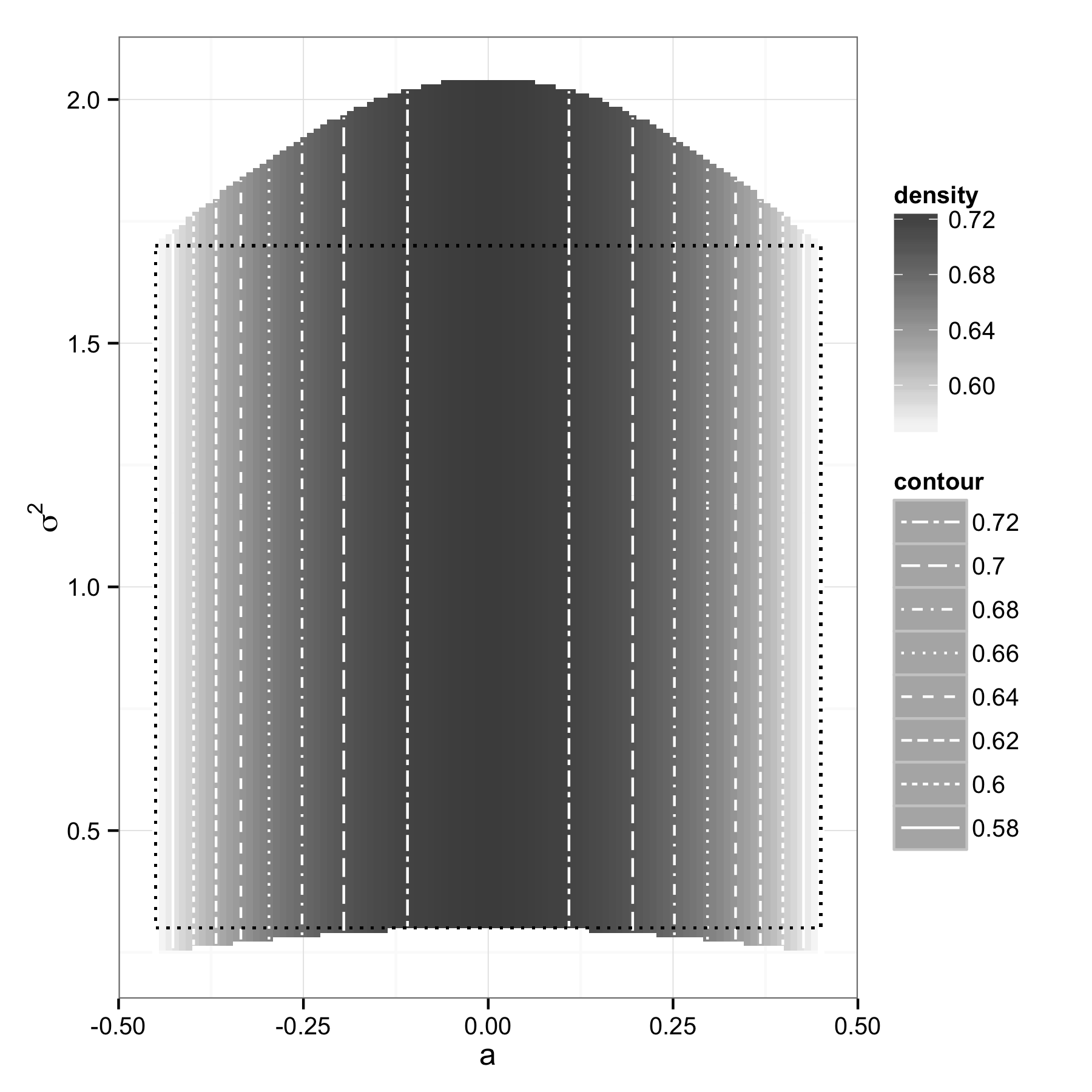
Figure S3: Prior on $\theta=(a,\sigma^{2})$ induced by an uniform prior on $\rho=(\rho_{1},\rho_{2})$, as given by equation (S5). The boundaries of the uniform prior on $\rho$ are computed using equations (S4) with $a^{-}=-0.43$, $a^{+}=0.43$, ${\sigma^{-}}^{2}=0.3$ and ${\sigma^{+}}^{2}=1.7$, which ensure that the prior induced on $\theta$ contains the rectangle $[a^{-},a^{+}]\times[{\sigma^{-}}^{2},{\sigma^{+}}^{2}]$ (black dotted line). Here, we have fixed the variance $\hat{\nu}_{x1}=(1+a^{2})\sigma^{2}$ and autocorrelation $\hat{\nu}_{x2}=\operatorname*{atanh}(a/(1+a^{2}))$ to their theoretical values and obtained the following uniform prior $(\rho_{1},\rho_{2})\sim U[(-0.493,0.294)\times(0.297,2.024)]$. Note that the prior induced on $\theta$ is rather uninformative.

An example of prior induced on $\theta$ is shown in Figure S3.

S4.2 Markov Chain Monte Carlo algorithm for estimating $\pi(\theta|x_{1:n})$

When inferring the parameters $\theta=(a,\sigma^{2})$ of $x_{1:n}\sim MA(1)$, the past white noise $u_{0}$ needs also to be inferred. However, since we used simulated data and were interested in the exact posterior of $\theta$ we simply fixed $u_{0}=0$ and used the likelihood of $x_{1:n}$ conditional on $u_{0}$ given by Marin and Robert (2007):

$$l^{c}(a,\sigma^{2}|x_{1:n},u_{0})\varpropto\sigma^{-n}\prod_{1}^{n}\exp(-\frac{\hat{u}_{t}^{2}}{2\sigma^{2}}),$$ (S6)

where the $\hat{u}_{t}(t>0)$ are given by the recursive formula:

$$\hat{u}_{t}=x_{t}-a\hat{u}_{t-1}.$$

We implemented a Metropolis-Hasting MCMC algorithm with a bivariate gaussian kernel proposal truncated to the natural support of $\theta$: $[-0.5,0.5]\times\mathbb{R}^{+}$ and with covariance matrix:

$$\Sigma_{\theta}=\left(\begin{array}[]{ccc}5\times 10^{-2}&5\times 10^{-4}\\ 5\times 10^{-4}&5\times 10^{-2}\end{array}\right).$$

leading to an acceptance rate of $\sim 20\%$. We ran and combined 6 chains for $2\times 10^{6}$ iterations, starting near the true parameter values.

S4.3 ABC^⋆ subsetting procedure

We considered the following subsets for given time series data $x_{1:n}$. First, autocorrelations in $x_{1:n}$ were ignored, leading to $s^{i}_{1}=x^{i}$, $i=1,\dotsc,n$ and $s_{2}=(x_{1},x_{2}),(x_{2},x_{3}),\dotsc$, $i=1,\dotsc,n$ for the variance and correlation test respectively. Second, we thinned $x_{1:n}$ to $s^{i}_{1a}=x^{2i-1}$ and $s^{i}_{1b}=x^{2i}$, $i=1,\dotsc,n/2$ for two variance tests, and used $s_{2a}=(x_{1},x_{2}),(x_{4},x_{5}),(x_{7},x_{8}),\dotsc$ and $s_{2b}=(x_{2},x_{3}),(x_{5},x_{6}),(x_{8},x_{9}),\dotsc$ and $s_{2c}=(x_{3},x_{4}),(x_{6},x_{7}),(x_{9},x_{10}),\dotsc$ for three correlation tests.

S4.4 Influence of the link function

The rate of change $\lvert\operatorname*{det}\partial\!\operatorname*{\mathcal{L}}\rvert$ is non-linear and may compromise the accuracy of point estimates of $\pi_{\operatorname*{a\!b\!c}}(\theta|x_{1:n})$. This is particularly so when $P_{x}(R|\rho)$ is broad so that $\lvert\operatorname*{det}\partial\!\operatorname*{\mathcal{L}}\rvert$ has considerable support to act on. To illustrate, we increased the sample size $n$ but did not re-calibrate $\tau^{+}_{k}$, expecting that $\hat{\theta}^{\operatorname*{MAP}}_{\operatorname*{a\!b\!c}}$ is increasingly inaccurate as the power function plateaus at one. We ran ABC^⋆ for different pseudo data sets that increase from $n=m=500$ to $n=m=10^{5}$. The $\hat{\theta}^{\operatorname*{MAP}}_{\operatorname*{a\!b\!c}}$ was indeed increasingly inaccurate when the $\tau^{+}_{k}$ are not re-calibrated for each $m$ (light gray dots in Figure S4D). We repeated inference, now with the $\tau^{+}_{k}$ re-calibrated so that power peaks at $0.9$. There was no systematic difference between $\hat{\theta}^{\operatorname*{MAP}}_{\operatorname*{a\!b\!c}}$ and the exact MAP estimate (A6 met, dark gray dots in Figure S4D). The amount of data available controlled $\lvert\operatorname*{det}\partial\!\operatorname*{\mathcal{L}}\rvert$ and the calibrations ensured that the ABC^⋆ MAP estimate was very close to $\hat{\theta}^{\operatorname*{MAP}}$ (A6 met; Figure S4D-E).

S5 Advanced ABC^⋆ algorithms

S5.1 Markov Chain Monte Carlo algorithm (MCMC)

The MCMC algorithm follows from (Marjoram et al., 2003). Set initial values $\theta^{0}$, compute $y^{0}\sim\ell(\,\cdot\,|\theta^{0})$ and $z^{0}_{k}=T_{k}\big{(}s_{k}^{1:{{m}_{k}}}(y^{0}),s_{k}^{1:{{n}_{k}}}(x)\big{)}$ for all $k$. We suppose that $c^{-}_{k}\leq z^{0}_{k}\leq c^{+}_{k}$ for all $k$.

ABC^⋆-m1

If now at $\theta$, propose $\theta^{\prime}$ according to a proposal density $q(\theta\rightarrow\theta^{\prime})$.

ABC^⋆-m2

Simulate $y^{\prime}\sim\ell(\,\cdot\,|\theta^{\prime})$, extract $s_{k}^{1:{{m}_{k}}}(y^{\prime})$ for all $k=1,\dotsc,K$.

ABC^⋆-m3

Compute $z^{\prime}_{k}=T_{k}\big{(}s_{k}^{1:{{m}_{k}}}(y^{\prime}),s_{k}^{1:{{n}_{k}}}(x)\big{)}$ for all $k$.

ABC^⋆-m4

Accept $(\theta^{\prime},z^{\prime})$ with probability

$$\begin{split}&mh(\theta,z;\theta^{\prime},z^{\prime})=\\ &\quad\min\Bigg{\{}1\>,\frac{q(\theta^{\prime}\rightarrow\theta)}{q(\theta\rightarrow\theta^{\prime})}\times\frac{\pi(\theta^{\prime})}{\pi(\theta)}\times\prod_{k=1}^{K}\operatorname*{\mathds{1}}\{c^{-}_{k}\leq z_{k}^{\prime}\leq c^{+}_{k}\}\Bigg{\}},\end{split}$$

and otherwise stay at $(\theta,x)$. Return to ABC^⋆-m1.

Throughout, we used a Gaussian proposal kernel. Annealing procedures were added to the covariance matrix of the Gaussian proposal kernel and the tolerances $\tau^{-}_{k}$, $\tau^{+}_{k}$ during burn-in.

For the influenza time series example, we previously used a standard ABC MCMC algorithm with annealing schemes on the covariance matrix of a Gaussian proposal matrix and the tolerances. The covariance matrix was diagonal. For ABC^⋆, the calibrated $c^{-}_{k}$, $c^{+}_{k}$ were considerably smaller than those used previously in the standard ABC routine, and we were forced to improve the MCMC sampler. We estimated a more suitable covariance matrix for the proposal density from a sequence of pilot runs, and also employed an annealing scheme on the covariance matrix as well as the tolerances $\tau^{-}_{k}$, $\tau^{+}_{k}$.

S5.2 Sequential Importance sampling algorithm

This algorithm follows in analogy to the above from (Toni et al., 2008).

S6 Supplementary Figures

Figure S1: Lower bound of ABC true positives. The true positive ABC^⋆ samples among all accepted ABC^⋆ samples after completion of the algorithm are those $\theta$ for which $\rho=\operatorname*{\mathcal{L}}(\theta)$ is in the equivalence region $H_{1}$. We obtain from Bayes Theorem that the percentage of true positive ABC^⋆ samples is bounded below by $P_{x}(H_{1}|R)=1-P_{x}(H_{0}|R)\geq 1-\alpha/P_{x}(R)$. The lower bound on the probability of correctly rejecting a level-$\alpha$ equivalence test statistic (i. e. $1-P_{x}(H_{0}|R)$) is plotted as a function of the ABC^⋆ acceptance probability $P_{x}(R)$ for $\alpha=0.01$ (blue) and $\alpha=0.05$ (black). Since the ABC^⋆ acceptance probability rarely exceeds $20\%$, we fix $\alpha=0.01$. In this case, if the ABC^⋆ acceptance probability is smaller than 2%, then the percentage of true positive ABC^⋆ samples could be as low as 50%

Figure S2: ABC^⋆ inference of $\sigma^{2}$ under calibrated tolerances $\tau^{-}<\tau^{+}$. Calibrated upper tolerance $\tau^{+}$ as a function of $m$ (dark gray). The dark gray $\hat{\theta}^{\operatorname*{MAP}}_{\operatorname*{a\!b\!c}}$ estimates in Figure LABEL:f:scaledFpowerF were obtained from an ABC^⋆ run with these calibrated upper tolerances. The light gray $\hat{\theta}^{\operatorname*{MAP}}_{\operatorname*{a\!b\!c}}$ estimates in Figure LABEL:f:scaledFpowerF were obtained from an ABC run with fixed upper tolerance (shown here also in light gray).

A

B

C

Figure S4: Link function and ABC^⋆ inference for the MA(1) model. (A) The link function (black) and $\lvert\operatorname*{det}\partial\!\operatorname*{\mathcal{L}}\rvert$ (gray) as a function of $a$. $\lvert\operatorname*{det}\partial\!\operatorname*{\mathcal{L}}\rvert$ increases to the left of $a_{0}=0.1$ (vertical grey line). (B) We increased the sample size $n$ but did not re-calibrate $\tau^{+}_{k}$, expecting that $\hat{\theta}^{\operatorname*{MAP}}_{\operatorname*{a\!b\!c}}$ is increasingly inaccurate as the power function plateaus at one. The $\hat{\theta}^{\operatorname*{MAP}}_{\operatorname*{a\!b\!c}}$ was indeed increasingly inaccurate when the $\tau^{+}_{k}$ are not re-calibrated for each $m$ (light gray dots). We repeated inference, now with the $\tau^{+}_{k}$ re-calibrated so that power peaks at $0.9$. There was no systematic difference between $\hat{\theta}^{\operatorname*{MAP}}_{\operatorname*{a\!b\!c}}$ and the exact MAP estimate (A6 met, dark gray dots). (C) Standard ABC posterior density (black contour) as described in the main text, with tolerances set so that ABC-r acceptance probability was 0.5%. Monte Carlo error becomes noticeable and otherwise ABC approximation is comparable to that of ABC^⋆.

A

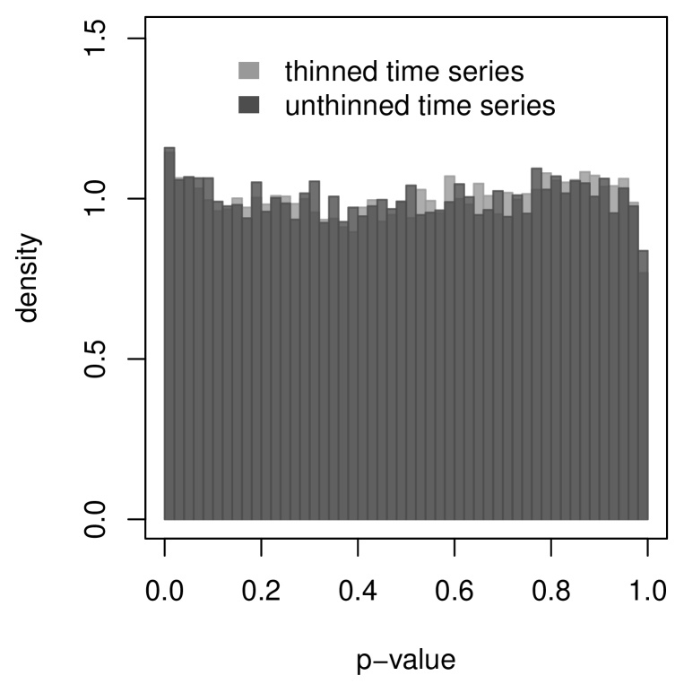
B

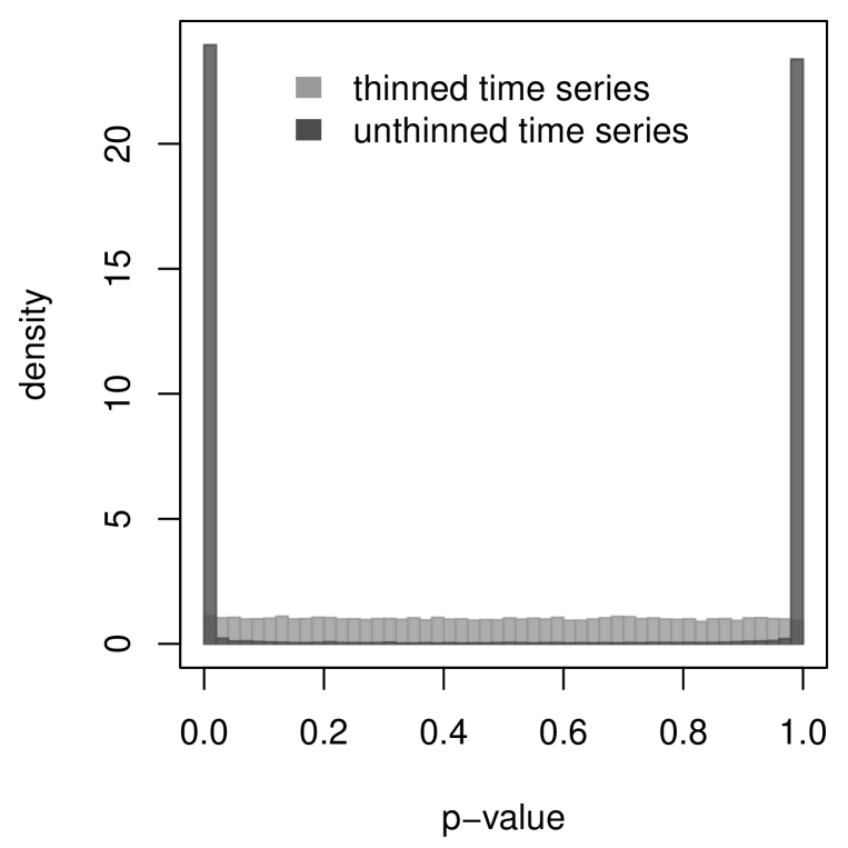
C

D

Figure S5: ABC self-assessment for ABC inference on the MA(1) model. We verified during ABC runtime that the test assumptions on the summary values are met. (A) To assess normality, we used the Shapiro-Francia test (Royston, 1993) to compute a p-value at every ABC iteration for each set of summary values. After runtime, the distribution of p-values was tested for departures from $\mathcal{U}(0,1)$. Histograms of p-values are shown for two cases: summary values set to the thinned time series (light gray) and to the time series without thinning (dark gray). (B) To assess if summary values are uncorrelated, we tested for non-zero partial autocorrelations (Box et al., 2011). Histograms are shown for the same two cases. Summary values can be considered uncorrelated only after thinning. Further, we evaluated if the link function can be numerically reconstructed from ABC output with local polynomial regressions. (C) The first dimension of the reconstructed link function $\hat{\operatorname*{\mathcal{L}}}_{1}$ (gray) and true link function $\operatorname*{\mathcal{L}}_{1}$ (black, dashed-dotted, on the sides), with added level set $\operatorname*{\mathcal{L}}_{1}^{-1}(\rho_{1}^{\star})$ (white). (D) The second dimension of the reconstructed link function $\hat{\operatorname*{\mathcal{L}}}_{2}$ (gray) and true link function $\operatorname*{\mathcal{L}}_{2}$ (black, dashed-dotted, on the sides), with added level set $\operatorname*{\mathcal{L}}_{2}^{-1}(\rho_{1}^{\star})$ (white).

Table S1: SEIIRS model parameters, priors, and standard ABC and ABC^⋆ posterior densities

	description	prior density	mean$\pm$std. dev., 95% conf. interval of
			standard ABC	ABC⋆
			posterior density	posterior density
			$\theta_{0}=(R_{0},1/\gamma,\omega)=(3.5,10,0.08)$
$R_{0}$	Basic reproductive	$\mathcal{U}(1,8)$	3.74$\pm$0.39, [3.01, 4.37]	3.51$\pm$0.02, [3.47, 3.54]
	number
$1/\phi$	Avg incubation	0.9 §
	period [day]
$1/\nu$	Avg infectiousness	1.8 §
	period [day]
$1/\gamma$	Avg duration	$\mathcal{U}(2,30)$	11.1$\pm$1.58, [8.15, 13.76]	9.93$\pm$0.07, [9.79, 10.07]
	of immunity [year]
$\omega$	Reporting rate	$\mathcal{U}(0,1)$	0.092$\pm$0.02,	0.0799$\pm 0.0004$,
			[0.058, 0.133]	[0.0791, 0.0808]
$N^{\scriptscriptstyle\downarrow}$	Size of sink	$\approx 15\times$106
	population	varies in time†
$N^{\scriptscriptstyle\circlearrowright}$	Size of source	$\mathcal{U}(1,10)$	∗	∗
	population	$\times$108
$\mu^{\scriptscriptstyle\downarrow}$	Birth/death rate of	fixed†
	sink population
$\mu^{\scriptscriptstyle\circlearrowright}$	Birth/death rate of	1/50 ¶
	source population,
	[1/year]
$\varphi^{\scriptscriptstyle\downarrow}$	Seasonal forcing of	$\mathcal{U}(0.07,0.6)$	∗	∗
	${\beta^{{\scriptscriptstyle\downarrow}}_{t}}$
$\varphi^{\scriptscriptstyle\circlearrowright}$	Seasonal forcing of	$\mathcal{U}(0,0.03)$	∗	∗
	${\beta^{{\scriptscriptstyle\circlearrowright}}_{t}}$
$m^{\scriptscriptstyle\downarrow}$	Number of travelers	$\mathcal{U}(3,15)$	∗	∗
	visiting the sink	$\times 10^{6}$ †
	population†
$m^{\scriptscriptstyle\circlearrowright}$	Fraction of $\hat{I}^{\scriptscriptstyle\circlearrowright}$ re-	$\mathcal{U}(0,0.1)$	∗	∗
	seeding the source
	population
$M^{\scriptscriptstyle\circlearrowright}$ in the analogue of (LABEL:e:classofmodels) for the source population is defined by $M^{\scriptscriptstyle\circlearrowright}=m^{\scriptscriptstyle\circlearrowright}\hat{I}^{\scriptscriptstyle\circlearrowright}$ where $\hat{I}^{\scriptscriptstyle\circlearrowright}$ is the
number of infected individuals at disease equilibrium in the source. †Fixed to demographic data
http://statline.cbs.nl. Number of travellers encompass annual records. §Fixed to match influenza
A (H3N2)’s estimated generation time ¶Assuming an average lifespan of 60 years, adjusted by
net fertility rate in SE Asia ∗For the simulated data set, these parameters were fixed to the
values reported in Figure LABEL:f:SEIIRS_datasets.

A

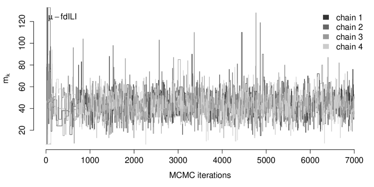
B

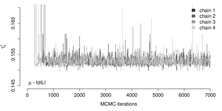
Figure S6: ABC inference on the influenza A (H3N2) data on simulated data - calibrations. ABC^⋆ inference based on the summary values in Figure LABEL:f:SEIIRS_datasets. TOST test statistics were used based on the distribution of the summary vales, and MCMC chains were run for 10.000 iterations. The free ABC parameters were re-calibrated at every iteration because the TOST also depends on the standard deviation of the summary values. (A) Calibrated $m_{k}$ and (B) calibrated $\tau^{+}_{k}$ for four MCMC chains that were run in parallel from overdispersed starting values.

References

• Berger and Hsu (1996) Berger, R. and J. Hsu (1996). Bioequivalence trials, intersection-union tests and equivalence confidence sets. Statistical Science 11(4), 283–319.
• Box et al. (2011) Box, G., G. Jenkins, and G. Reinsel (2011). Time series analysis: forecasting and control. Wiley.
• Hotelling (1953) Hotelling, H. (1953). New light on the correlation coefficient and its transforms. Journal of the Royal Statistical Society. Series B (Methodological) 15(2), 193–232.
• Lehmann and Romano (2005) Lehmann, E. and J. Romano (2005). Testing statistical hypotheses. Springer.
• Marin and Robert (2007) Marin, J.-M. and C. P. Robert (2007). Bayesian core: a practical approach to computational Bayesian statistics. Springer.
• Marjoram et al. (2003) Marjoram, P., J. Molitor, V. Plagnol, and S. Tavaré (2003). Markov Chain Monte Carlo without likelihoods. Proceedings of the National Academy of Sciences USA 100(26), 15324–15328.
• Owen (1965) Owen, D. (1965). A special case of a bivariate non-central t-distribution. Biometrika 52(3/4), 437–446.
• Royston (1993) Royston, P. (1993). A pocket-calculator algorithm for the Shapiro-Francia test for non-normality: An application to medicine. Statistics in Medicine 12(2), 181–184.
• Schuirmann (1981) Schuirmann, D. (1981). On hypothesis testing to determine if the mean of a normal distribution is contained in a known interval. Biometrics 37(617), 137.
• Toni et al. (2008) Toni, T., D. Welch, N. Strelkowa, A. Ipsen, and M. P. H. Stumpf (2008). Approximate Bayesian computation scheme for parameter inference and model selection in dynamical systems. Journal of The Royal Society Interface 6(31), 187–202.