Dynamic Covariance Models for Multivariate Financial Time Series

Abstract

The accurate prediction of time-changing covariances is an important problem in the modeling of multivariate financial data. However, some of the most popular models suffer from a) overfitting problems and multiple local optima, b) failure to capture shifts in market conditions and c) large computational costs. To address these problems we introduce a novel dynamic model for time-changing covariances. Over-fitting and local optima are avoided by following a Bayesian approach instead of computing point estimates. Changes in market conditions are captured by assuming a diffusion process in parameter values, and finally computationally efficient and scalable inference is performed using particle filters. Experiments with financial data show excellent performance of the proposed method with respect to current standard models.

1 Introduction

Univariate financial returns are heteroscedastic, that is, the volatility or standard deviation of financial returns is not constant, but changes with time (Cont, 2001). Several univariate models have been proposed to capture this property. The best known are the Autoregressive Conditional Heteroscedasticity model (ARCH) (Engle, 1982) and its extension, the Generalized Autoregressive Conditional Heteroscedasticity model (GARCH) (Bollerslev, 1986). This topic has recently received attention in the machine learning community, with the development of copula processes (Wilson & Ghahramani, 2010) and heteroskedastic Gaussian processes (Lázaro-Gredilla & Titsias, 2011).

Multivariate financial returns exhibit similar patterns. Moreover, besides time-dependent volatilities, they also display time-dependent correlations (Patton, 2006). Covariances are the product of variances and correlations. Therefore these temporal dependencies are likewise present in covariance matrices. To capture these properties Engle & Kroner (1995) proposed a multivariate extension of GARCH called BEKK, based on synthesized work of Baba, Engle, Kraft, and Kroner. An alternative to BEKK are stochastic volatility models, including recent non-parametric models based on generalized Wishart processes (Wilson & Ghahramani, 2011; Fox & Dunson, 2011). In practice BEKK performs similarly to the generalized Wishart processes for modeling financial data. However, BEKK is known to suffer from the following disadvantages:

1. The parameters of BEKK are usually fit by maximum likelihood. The large number of parameters in BEKK and local maxima in the likelihood function often lead to overfitting.

2. The parameter values in BEKK are constant. However, financial markets are dynamic and market conditions change with time. BEKK does not naturally capture these shifts in market conditions.

3. Finally, maximum likelihood fit of the parameters of BEKK involves solving a non-linear optimization process which is computationally expensive and infeasible in high-dimensions.

To address the difficulties mentioned above, we present a novel dynamic model for describing time-dependent covariance matrices which extends BEKK as follows: Instead of computing point estimates, as in BEKK, we follow a fully Bayesian approach and compute posterior probabilities for the parameter values. This reduces the detrimental effect of multiple maxima in the likelihood function and limits overfitting problems. In addition to this, the new dynamic model incorporates a diffusion process for parameter values. At each point in time, every parameter is slightly modified by a random perturbation. These perturbations allow the model to adapt its parameters to changes in market conditions. Finally, Bayesian inference is performed using a regularized auxiliary particle filter (Liu & West, 1999). This technique is very efficient in terms of computational cost and allows our method to scale up to high dimensions.

The performance of the new dynamic model for time-changing covariance matrices is evaluated in a series of experiments with real financial returns. The proposed model is compared with the standard BEKK model and a variant of BEKK that assumes multivariate Student’s $t$ innovations. Finally, we compare the proposed model against the generalized Wishart processes. Overall, the new dynamic model for time-varying covariance matrices obtains the best predictive performance.

The rest of the document is organized as follows: Section 2 describes standard heteroscedastic models such as GARCH and BEKK. Section 3 introduces our novel Bayesian Multivariate Dynamic Covariance model (BMDC). Section 4 reviews current models for dynamic covariances in machine learning. Section 5 describes the particle filter algorithm for making inference in BMDC. Experiments comparing BMDC with BEKK are included in Section 6 and additional experiments comparing BMDC with the generalized Wishart process are included in Section 7. Finally, Section 8 contains the conclusions of the study.

2 Review of GARCH and BEKK

GARCH is the standard time-series model for univariate heteroscedastic data. GARCH assumes Gaussian noise or innovations and produces a sequence of time-varying variances $\sigma_{t}^{2}$ that follow an Autoregressive and Moving Average (ARMA) process with autoregression on $p$ previous variance values and moving average on $q$ previous squared time-series values:

$$x_{t} \sim\mathcal{N}(0,\sigma_{t}^{2})\,,$$ (1)

$$\sigma_{t}^{2} =\alpha_{0}+\sum_{j=1}^{q}\alpha_{j}x_{t-j}^{2}+\sum_{i=1}^{p}\beta_{i}\sigma_{t-i}^{2}\,.$$ (2)

The generative model is flexible and can produce a variety of clustering behavior of high and low volatility periods for different settings of the model coefficients, $\alpha_{1},\ldots,\alpha_{p}$ and $\beta_{1},\ldots,\beta_{q}$. Maximum likelihood is used to learn these coefficients with $p$ and $q$ usually set to 1 to reduce overfitting problems.

BEKK (Engle & Kroner, 1995) is a popular multivariate extension of GARCH, where the dynamic covariance matrix for the data follows an ARMA process:

$$\mathbf{x}_{t} \sim\mathcal{N}(0,\bm{\Sigma}_{t})\,,$$ (3)

$$\bm{\Sigma}_{t} =\mathbf{C}^{\top}\mathbf{C}+\sum_{j=1}^{q}\mathbf{B}_{j}^{\top}\mathbf{x}_{t-j}\mathbf{x}_{t-j}^{\top}\mathbf{B}_{j}+\sum_{i=1}^{p}\mathbf{A}_{i}^{\top}\bm{\Sigma}_{t-i}\mathbf{A}_{i}$$ (4)

where $\mathbf{A}_{i}$ and $\mathbf{B}_{j}$ are $d\times d$ coefficient matrices for $d$ dimensional data and $C$ is a triangular matrix with $d(d+1)/2$ non-zero entries. Therefore BEKK($p$,$q$) is a highly parameterized model with a total of $(p+q)d^{2}+d(d+1)/2$ parameters.

Restricted versions of BEKK are used in practice to mitigate overfitting problems. The order parameters $p$ and $q$ are set to 1 and the matrices $\mathbf{A}_{1}$ and $\mathbf{B}_{1}$ are constrained to be diagonal. The expression for $\bm{\Sigma}_{t}$ is now

$$\bm{\Sigma}_{t} =\mathbf{C}^{\top}\mathbf{C}+\mathbf{B}\mathbf{x}_{t-1}\mathbf{x}_{t-1}^{\top}\mathbf{B}+\mathbf{A}\bm{\Sigma}_{t-1}\mathbf{A}\,.$$ (5)

This diagonal BEKK model (Engle & Kroner, 1995) has only $2d+d(d+1)/2$ parameters. We will use this model as the baseline for comparison because it often has better predictive performance than other versions of BEKK and its computational cost is also lower. Subsequent references to BEKK will mean the diagonal BEKK model shown in (5).

Standard BEKK has Gaussian innovations. However, there is strong evidence that financial returns are heavy-tailed. Harvey et al. (1992) and Fiorentini et al. (2003) incorporate heavy-tails in BEKK by modeling $\mathbf{x}_{t}$ using a multivariate Student’s $t$ distribution with $\nu$ degrees of freedom, zero mean, and scale matrix $\mathbf{S}_{t}$:

$$\mathbf{x}_{t} \sim\mathcal{S}(\nu,0,\mathbf{S}_{t})\,,$$ (6)

$$p(\mathbf{x}_{t}) =\frac{\Gamma[(\nu+d)/2][1+\frac{1}{\nu}\mathbf{x}_{t}^{\top}\mathbf{S}_{t}^{-1}\mathbf{x}_{t}]^{-(\nu+d)/2}}{\Gamma(\nu/2)(\nu\pi)^{d/2}\mathop{\left|\mathbf{S}_{t}\right|}^{1/2}}\,,$$ (7)

$$\mathbf{S}_{t} =\frac{\nu-2}{\nu}\bm{\Sigma}_{t}\,.$$ (8)

The degrees of freedom, $\nu$, should be larger than two for $\mathbf{x}_{t}$ to have a well defined covariance. Finally, the expression for $\mathbf{S}_{t}$ ensures the expected covariance of $\mathbf{x}_{t}$ is $\bm{\Sigma}_{t}$. We will refer to the diagonal BEKK model with Student’s $t$ innovations as BEKK-T.

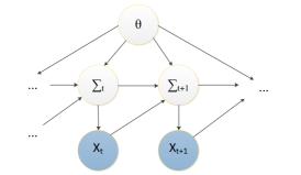
Figure 1: Left, graphical model for BEKK. The parameters $\theta=(\mathbf{A},\mathbf{B},\mathbf{C})$ are in this case static. Right, graphical model for BMDC with time-varying parameters $\mathbf{\theta}_{t}=(\mathbf{A}_{t},\mathbf{B}_{t},\mathbf{C}_{t})$. BMDC naturally captures changes in market conditions.

3 Bayesian Multivariate Dynamic Covariance Models

A major limitation of BEKK is that the parameter matrices $\mathbf{A}$, $\mathbf{B}$ and $\mathbf{C}$ are assumed to be constant. This is unrealistic for financial data, where market fundamentals are expected to change with time. A heuristic solution is to run BEKK over different windows of historical data. The problem is then how to choose the window size, with trade-offs between noisy but reactive estimates of the model parameters for small windows and more stable but constant parameter estimates for large windows.

As a more principled approach to capture changes in market dynamics, we introduce a novel Bayesian Multivariate Dynamic Covariance model (BMDC) with time-varying parameters. For this, we replace (5) by

$$\bm{\Sigma}_{t} =\mathbf{C}_{t}^{\top}\mathbf{C}_{t}+\mathbf{B}_{t}\mathbf{x}_{t-1}\mathbf{x}_{t-1}^{\top}\mathbf{B}_{t}+\mathbf{A}_{t}\Sigma_{t-1}\mathbf{A}_{t}\,.$$ (9)

where $\mathbf{C}_{t}$, $\mathbf{B}_{t}$ and $\mathbf{A}_{t}$ are time-dependent matrices. Let $\mathbf{\theta}=\{\mathbf{A},\mathbf{B},\mathbf{C}\}$ and $\mathbf{\theta}_{t}=\{\mathbf{A}_{t},\mathbf{B}_{t},\mathbf{C}_{t}\}$. Figure 1 shows the corresponding graphical models for BEKK and BMDC.

In BMDC, the dynamic parameters in $\theta_{t}$ follow a diffusion process in which $\theta_{t+1}$ is obtained by adding a small random perturbation to the parameters in $\theta_{t}$. Since $\mathbf{A}_{t}$ and $\mathbf{B}_{t}$ are diagonal, let $\mathbf{a}_{t}$ and $\mathbf{b}_{t}$ denote $d$-dimensional vectors with the diagonal elements of these matrices and let $\mathbf{c}_{t}$ be the vector with the upper triangular terms of $\mathbf{C}_{t}$. Then we specify the following diffusion process for $\mathbf{a}_{t}$, $\mathbf{b}_{t}$ and $\mathbf{c}_{t}$:

$$\mathbf{a}_{t} \sim\mathcal{N}(\mathbf{a}_{t-1},\alpha^{2}I)\,,$$ (10)

$$\mathbf{b}_{t} \sim\mathcal{N}(\mathbf{b}_{t-1},\beta^{2}I)\,,$$ (11)

$$\mathbf{c}_{t} \sim\mathcal{N}(\mathbf{c}_{t-1},\gamma^{2}I)\,,$$ (12)

$$\alpha \sim\mathcal{N}(\kappa,\tau)\,,\quad\beta\sim\mathcal{N}(\kappa,\tau)\,,\quad\gamma\sim\mathcal{N}(\kappa,\tau)\,.$$ (13)

where the hyper-parameters $\alpha$, $\beta$ and $\gamma$ control the amount of drift in the system. In practice, vague priors are chosen for the value of these hyper-parameter, with mean prior drift set to zero, $\kappa=0$. $\tau$ was set to $0.005^{2}$ so that $A$, $B$ and $C$ can move up to $0.005\sqrt{N}$, where $N$ is the number of observations. Other values of $\tau$ were tried with little difference in predictive performance. The prior for the initial state $\mathbf{a}_{0}$, $\mathbf{b}_{0}$ and $\mathbf{c}_{0}$ is also vague, taking into account the constraint $(|\mathbf{A}_{0}\mathbf{A}_{0}|+|\mathbf{B}_{0}\mathbf{B}_{0}|)\leq 1$ so that $\bm{\Sigma}_{t}$ does not diverge, where $|\cdot|$ calculates the determinant of a matrix.

An important property of BMDC is that its predictive distribution is heavy-tailed. This is desirable as financial time series have fat tails (Cont, 2001). The heavy-tails in the predictions of BMDC arise because

$$p(\mathbf{x}_{t}^{\star}|\bm{\Sigma}_{t-1},\mathbf{x}_{t-1})=\int p(\mathbf{x}_{t}^{\star}|\bm{\Sigma}_{t})p(\bm{\Sigma}_{t}|\bm{\Sigma}_{t-1},\mathbf{x}_{t-1})d\bm{\Sigma}_{t}\,.$$ (14)

where the distribution of $\bm{\Sigma}_{t}|\bm{\Sigma}_{t-1},\mathbf{x}_{t-1}$ is obtained by integrating (9) with respect to the posterior for $\theta_{t}=(\mathbf{A}_{t},\mathbf{B}_{t},\mathbf{C}_{t})$. Since $p(\mathbf{x}_{t}^{\star}|\bm{\Sigma}_{t})$ is Gaussian, (14) is an infinite mixture of multivariate Gaussians and it will generally be heavy-tailed. This implies that the predictive density in the BMDC model will also have heavy tails.

In addition to BMDC, we propose a variant of this model with Student’s $t$ innovations, which we denote BMDC-T. In this case, a vague log-normal prior is placed on the parameter $\nu$ corresponding to the number of degrees of freedom of the Student’s $t$ innovations:

$$\log(\nu-2)\sim\mathcal{N}(0,\sigma_{\nu}^{2})\,.$$

4 Related Work

The GARCH and BEKK models described in Section 2 constitute the most popular family of volatility models. They are characterized by the latent covariance matrix $\bm{\Sigma}_{t}$ being dependent on both its most recent past value $\bm{\Sigma}_{t-1}$ and the previous time-series observation $\mathbf{x}_{t-1}$. Another class of models is the family of Stochastic Volatility models (Harvey et al., 1994; Chib et al., 2009; Gouriéroux et al., 2009; Philipov & Glickman, 2006). In this case, $\bm{\Sigma}_{t}$ is conditionally independent of $\mathbf{x}_{t-1}$ given its previous value $\bm{\Sigma}_{t-1}$. That is, graphically, in a stochastic volatility model there will be no arrow from node $\mathbf{x}_{t}$ to node $\bm{\Sigma}_{t+1}$ in the graphs shown in Figure 1. However, $\bm{\Sigma}_{t}$ will still be conditionally independent of $\bm{\Sigma}_{k}$ for $k<t-1$ and $k>t+1$ given $\bm{\Sigma}_{t+1}$ and $\bm{\Sigma}_{t-1}$. This latter condition does not hold in recent generalizations of these models based on generalized Wishart processes (GWP) (Fox & Dunson, 2011; Wilson & Ghahramani, 2011). In this case, there are dependencies between all the latent covariance matrices and the model can produce complex non-linear patterns in the evolution of covariance matrices. However, it is not clear that such flexibility is necessary for successfully modeling financial data. Our experiments show that BMDC outperforms GWP on this task, which confirms that this is not the case.

5 Inference with Particle Filters

Inference for the proposed Bayesian models is performed using particle filters (Doucet et al., 2001). Particle filters seem a natural choice to do online inference for these non-linear and non-Gaussian sequential models. BMDC has Gaussian likelihoods, but is non-linear in the model parameters $\mathbf{A}_{t}$, $\mathbf{B}_{t}$ and $\mathbf{C}_{t}$. Furthermore, particle filters can easily accommodate models with Student’s $t$ innovations, such as BMDC-T.

We analyzed several particle filtering methods, including Resample-Move (Gilks & Berzuini, 2001), Regularized Sequential Importance Sampling (Musso et al., 2001), Regularized Sequential Importance Resampling (Gordon et al., 1993), and Regularized Auxiliary Particle Filter (RAPF) (Liu & West, 1999) to perform inference in the proposed models. RAPF, a hybrid version of regularized (Musso et al., 2001) and auxiliary particle filters (Pitt & Shephard, 1999), exhibited the best performance in terms of predictiveness. This agrees with results given by Casarin & Marin (2009). An implementation of the RAPF for BMDC is shown in Algorithm 1. A detailed description of the algorithm is given in the following paragraph.

Liu & West (1999) introduced the RAPF, which combines the Regularized Particle Filter with the Auxiliary Particle Filter. The Regularized Particle Filter allows joint inference of the diffusion hyper-parameters, $\alpha$, $\beta$, $\gamma$, and the hidden states, $\mathbf{A}_{t}$, $\mathbf{B}_{t}$ and $\mathbf{C}_{t}$. This method explores the posterior distribution of the model parameters by taking kernelized steps sequentially, thereby avoiding particle death. The shrinkage kernel, (17) and (19), avoids over-dispersion problems in standard Regularized Particle Filters and improves prediction accuracy. The shrinkage kernel retains the previous mean, while the posterior variance does not diverge:

$$\mathbb{E}(\mathbf{\theta}_{t}) =\bar{\mathbf{\theta}}_{t-1}$$ (15)

$$\operatorname{Cov}(\mathbf{\theta}_{t}) =a^{2}V_{t}+(1-a^{2})V_{t}=V_{t}$$ (16)

The Auxiliary Particle Filter part of the algorithm can be viewed as interchanging the importance sampling and resampling steps in traditional particle filters such as Sequential Importance Resampling. The resampling, (18), is performed on $\mu_{t}^{i}$, which are predicted estimates of $\bm{\Sigma}_{t}$ given particles from the previous time step. Importance samples are then generated from the resampled point estimates. Particle diversity is maintained if the predicted estimates from the previous step are close to the true state. Auxiliary particle filtering is less sensitive to outliers and works well when the predicted estimates are good representations of the unknown states.

There are two algorithm parameters in Algorithm 1. The number of particles $N$ and the shrinkage parameter $a$. We followed Liu & West (1999) and fixed $a=0.95$. This leads to a little shrinkage and avoids parameter variance exploding. If shrinkage is large ($a=0$) then the particle filter would propose from a less heavy-tailed proposal distribution, with the parameters set to be their empirical means from the previous step. When the empirical means are inaccurate, then the proposed particles will not be representative of the hidden state. The number of particles, $N$, can affect the accuracy of the predictions, and is investigated in Section 6. The computational complexity of the algorithm is $O(Nd^{3})$ at each time step, where $d$ is the dimension of the data, since importance sampling at each step requires $N$ likelihood computations, each one with cost $O(d^{3})$.

6 Experiments for BMDC vs. BEKK

We evaluated the performance of BMDC, BEKK and their Student’s $t$ variants in several experiments with multivariate financial time series. The high computational cost of BEKK limited the maximum number of different financial assets in each of the analyzed series to five. We considered daily foreign exchange (FX) and daily equity returns, as well as intraday FX returns. The daily FX time series contain a total of 780 returns from January 2008 to January 2011. The daily equity time series contain 3000 returns from Jan 2000 to Dec 2011. The intraday FX time series consist of 5000 five-minute returns, which covered approximately the first six trading months of 2008. The price data were pre-processed to eliminate spurious prices. In particular, we eliminated prices corresponding to times when markets were closed or not liquid. All the time series were standardized to have zero mean and unit standard deviation.

To illustrate the usefulness of considering time-varying parameter values, we compared the predictive performance of BMDC and BMDC-T with BEKK and BEKK-T. In addition, we compared the execution times of i) the RAPF method used by the Bayesian models and ii) the maximum likelihood estimation method used by the BEKK models. Finally, we studied the sensitivity of RAPF to the number of particles used.

The performance of each method is measured in terms of the predictive log-likelihood on the first return out of the training set. During the experiments, each method receives an initial time-series of length 50. The different methods are trained on that data and then a one-step forward prediction is made. The predictive log-likelihood is evaluated on the next observation out of the training set. Then the training set is augmented with the new observation and the training and prediction steps are repeated again. The process is repeated sequentially until no further data is received.

Table 1: Avg. Predictive Likelihood on Daily FX Data

Dataset	BEKK	BEKK-T	BMDC	BMDC-T
EUR	$-1.47$	$-1.40$	$-1.36$	$\mathbf{-1.36}$
AUD	$-1.32$	$-1.29$	$-1.25$	$\mathbf{-1.25}$
BRL	$-1.18$	$-1.16$	$-1.15$	$\mathbf{-1.14}$
GBP	$-1.33$	$-1.33$	$\mathbf{-1.31}$	$\mathbf{-1.31}$
CHF	$-1.44$	$-1.45$	$-1.37$	$\mathbf{-1.37}$
AUD,JPY	$-2.62$	$\mathbf{-2.56}$	$-2.57$	$\mathbf{-2.56}$
EUR,CHF	$-2.15$	$\mathbf{-2.04}$	$-2.07$	$-2.05$
EUR,GBP	$-2.47$	$-2.44$	$\mathbf{-2.41}$	$\mathbf{-2.41}$
BRL,EUR	$-2.52$	$-2.46$	$\mathbf{-2.43}$	$\mathbf{-2.42}$
ZAR,AUD	$-2.34$	$-2.27$	$\mathbf{-2.27}$	$\mathbf{-2.26}$
CHF,EUR,JPY	$-3.75$	$-3.56$	$-3.27$	$\mathbf{-3.20}$
JPY,AUD,NZD	$-6.82$	$-3.77$	$-3.24$	$\mathbf{-3.20}$
BRL,AUD,ZAR	$-3.38$	$-3.31$	$-3.25$	$\mathbf{-3.23}$
TWD,JPY,KRW	$-7.43$	$-5.71$	$-3.61$	$\mathbf{-3.57}$
CAD,MXN,BRL	$-3.43$	$-3.33$	$-3.19$	$\mathbf{-3.17}$
JPY,AUD,EUR,CHF	$-4.71$	$-4.75$	$-4.21$	$\mathbf{-4.11}$
BRL,MXN,CAD,AUD	$-4.67$	$-4.30$	$-4.09$	$\mathbf{-4.01}$
BRL,ZAR,AUD,NOK	$-4.62$	$-4.46$	$-4.22$	$\mathbf{-4.19}$
JPY,AUD,GBP,EUR,CHF	$-8.94$	$-6.57$	$-5.31$	$\mathbf{-5.16}$
BRL,MXN,CAD,AUD,ZAR	$-5.51$	$-5.41$	$-5.14$	$\mathbf{-5.01}$
NZD,AUD,JPY,EUR,SEK	$-6.33$	$-5.58$	$-4.90$	$\mathbf{-4.80}$

Table 2: Avg. Predictive Likelihood on Intraday FX Data

Dataset	BEKK	BEKK-T	BMDC	BMDC-T
AUDJPY	$-1.16$	$\mathbf{-1.09}$	$\mathbf{-1.09}$	$\mathbf{-1.09}$
AUDUSD	$-1.19$	$\mathbf{-1.14}$	$\mathbf{-1.15}$	$\mathbf{-1.15}$
EURAUD	$-1.15$	$\mathbf{-1.10}$	$\mathbf{-1.10}$	$\mathbf{-1.10}$
EURCHF	$-1.25$	$\mathbf{-1.20}$	$-1.22$	$-1.22$
EURCZK	$-1.26$	$\mathbf{-1.11}$	$-1.16$	$-1.14$
EURGBP,EURUSD	$-2.57$	$\mathbf{-2.49}$	$-2.51$	$\mathbf{-2.50}$
EURHUF,GBPJPY	$-2.33$	$-2.20$	$-2.22$	$\mathbf{-2.17}$
EURJPY,GBPUSD	$-2.37$	$\mathbf{-2.27}$	$-2.29$	$\mathbf{-2.27}$
EURNOK,NZDUSD	$-2.88$	$\mathbf{-2.18}$	$-2.25$	$-2.20$
EURSEK,USDCAD	$-2.45$	$\mathbf{-2.32}$	$-2.35$	$\mathbf{-2.32}$
EURUSD,USDCHF,USDJPY	$-3.57$	$-3.28$	$-3.26$	$\mathbf{-3.18}$
GBPJPY,USDJPY,USDMXN	$-3.17$	$-2.56$	$-2.52$	$\mathbf{-2.41}$
GBPUSD,USDMXN,USDNOK	$-3.14$	$-2.84$	$-2.79$	$\mathbf{-2.65}$
NZDUSD,USDNOK,USDSEK	$-3.63$	$-3.41$	$-3.15$	$\mathbf{-3.07}$
USDCAD,USDSEK,USDSGD	$-3.78$	$-3.67$	$-3.69$	$\mathbf{-3.61}$

6.1 Results for BMDC vs. BEKK

Table 1 shows the average predictive log-likelihood for BEKK, BEKK-T, BMDC and BMDC-T on twenty-one daily FX time series sorted by the dimensionality of the data. The method with the best predictive performance on each time series is highlighted in bold. Corresponding results are shown in tables 2 and 4 for fifteen intraday FX and thirty daily equity time series respectively. Overall, the best performing method is BMDC-T followed by BEKK-T and BMDC. The worst performing method is BEKK.

We perform a statistical test to determine whether differences among BEKK, BEKK-T, BMDC and BMDC-T are significant. These methods are compared to each other using the multiple comparison approach described by Demšar (2006). In this comparison framework, all the methods are ranked according to their performance on different tasks. Statistical tests are then applied to determine whether the differences among the average ranks of the methods are significant. In our case, each of the $66=21+15+30$ datasets analyzed represents a different task. A Friedman rank sum test rejects the hypothesis that all methods have equivalent performance at $\alpha=0.05$. Pairwise comparisons between all the methods with a Nemenyi test at a 95% confidence level are summarized in Figure 3. The methods whose average ranks across datasets differ more than a critical distance (segment labeled CD in the figure) show significant differences in performance at this confidence level. The Nemenyi test confirms that BMDC-T is superior to all the other methods. Additionally, the dynamic methods are superior to their static counterparts with BMDC outperforming BEKK and BMDC-T beating BEKK-T. Finally, BMDC is not statistically different from BEKK-T.

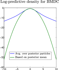
Figure 2: The log predictive density using the full posterior is much flatter and thereby heavy-tailed than the one using only the posterior mean for BMDC

The plot in Figure 3 shows that the heavy-tailed models BMDC-T and BEKK-T perform better than the non-heavy-tailed BEKK. Although BMDC assumes a Gaussian likelihood its posterior predictive distribution is heavy-tailed, as discussed in Section 3. Figure 2 confirms this by showing the logarithm of the posterior predictive density produced by BMDC on a particular instance of the analyzed time series. To produce this plot, we evaluated $p(\mathbf{x}_{t}|\theta_{t},\bm{\Sigma}_{t-1},\mathbf{x}_{t-1})$ on a grid of values for one dimension of $\mathbf{x}_{t}$, averaging over the available particles which approximate the posterior distribution of $\theta_{t}$ and $\bm{\Sigma}_{t-1}$. This is compared to the plot obtained by evaluating $p(\mathbf{x}_{t}|\theta_{t},\bm{\Sigma}_{t-1},\mathbf{x}_{t-1})$ on the posterior mean estimate of $\theta_{t}$ and $\bm{\Sigma}_{t-1}$, which is approximated by the empirical mean computed across all the particles.

Figure 3: All to all comparison between BMDC-T, BMDC, BEKK-T and BEKK via a Nemenyi test. The horizontal axis indicates the average rank of each method on the 66 analyzed time series. If the differences in average ranks are larger than the critical distance (length of the segment labeled CD) then differences in performance are statistically significant at $\alpha=0.05$. In this case, the differences in rank between BMDC-T and all the other methods are significant.

To understand the superior performance of BMDC relative to BEKK, we plot the average predictive log-likelihood of each method against the number of observations in Figure 4. The plot shows typical average predictive log-likelihood for a $3D$ Daily FX time series. BMDC-T is clearly the most predictive method for any number of observations. BEKK and BEKK-T underperform BMDC and BMDC-T early on, when relatively few observations are available to fit the models. These two methods are susceptible to overfitting at early stages (especially BEKK-T in this case). With more data, BEKK-T is less susceptible to overfitting and outperforms BEKK. However, BEKK and BEKK-T still perform worse than BMDC and BMDC-T when the amount of training data increases. This confirms that BMDC and BMDC-T are better models for dynamic covariances in financial data, not only because BEKK and BEKK-T suffer from initial overfitting problems. As a note of financial interest, the average predictive log-likelihood dips after 150 observations. This corresponds to the highly turbulent period near the end of 2008 with large swings in financial asset prices resulting in lower predictive log-likelihood.

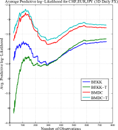
Figure 4: Avg. predictive log-Likelihood for each method over number of observations.

Table 3: Sensitivity in the average predictive log-likelihood of BMDC-T to the number of Particles used on Daily FX data. Execution times in minutes are shown in parentheses. Results of BEKK-T are shown for comparison.

Dataset	BEKK-T	N=1000	N=4000	N=9000	N=25000
1D	$-1.33$ $(71)$	$-1.32$ $(8)$	$-1.32$ $(20)$	$-1.32$ $(52)$	$\mathbf{-1.32}$ $(173)$
2D	$-2.56$ $(339)$	$-2.58$ $(8)$	$-2.56$ $(25)$	$\mathbf{-2.55}$ $(55)$	$-2.56$ $(176)$
3D	$-3.66$ $(478)$	$-3.24$ $(9)$	$-3.21$ $(29)$	$-3.20$ $(57)$	$\mathbf{-3.18}$ $(180)$
4D	$-4.52$ $(1003)$	$-4.25$ $(9)$	$-4.28$ $(30)$	$-4.20$ $(64)$	$\mathbf{-4.16}$ $(183)$
5D	$-5.95$ $(2971)$	$-5.60$ $(9)$	$-5.55$ $(32)$	$-5.53$ $(68)$	$\mathbf{-5.50}$ $(202)$
10D	$-$ $(-)$	$-9.01$ $(9)$	$-8.93$ $(45)$	$-7.96$ $(75)$	$\mathbf{-7.84}$ $(252)$
20D	$-$ $(-)$	$-20.04$ $(20)$	$-18.10$ $(37)$	$-17.27$ $(83)$	$\mathbf{-16.11}$ $(359)$

A major advantage of BMDC and BMDC-T with the RAPF method for Bayesian inference is scalability. Table 3 shows prediction sensitivity of the regularized particle filter to different number of particles and total execution times in minutes in parentheses for the BMDC-T model on the daily FX dataset with 780 observations, ordered by data dimension. BEKK-T predictions and execution times are also provided for comparison, except for datasets of ten or higher dimensions where BEKK-T failed to finish in a reasonable amount of time. BEKK-T was implemented using numerical optimization routines provided by Kevin Sheppard .

Clearly particle filtering is much faster than the numerical optimization of the log-likelihood function used by BEKK. In fact, particle filtering can be used for intraday trading and hedging since each sequential update is on the order of $68*60/780\approx 5$ seconds for five dimensional time series with $N=9000$ particles. The computational cost of the particle filter is $O(Nd^{3})$ at each step, as described in Section 5. The computational cost for BEKK is $O(Ltd^{5})$ at each step, where $L$ denotes the average number of numerical iterations needed per cycle and $t$ is the length of the training data currently seen. The power $d^{5}$ in this cost originates because, at each iteration of the optimization process, BEKK has to compute the gradient of $\mathcal{O}(d^{2})$ parameters, where each gradient computation requires $\mathcal{O}(d^{3}t)$ operations. This cost makes BEKK infeasible for large datasets. In contrast, the cost of the RAPF at each step does not depend on $t$ and only scales as $\mathcal{O}(d^{3})$. This allows the RAPF to analyze long high-dimensional time series.

Table 3 also shows the sensitivity of the predictions of BMDC-T to the number of particles $N$. Increasing $N$ improves performance, but has relatively small effect for low dimensional datasets. For higher dimensions, that is, $d\geq 10$, improvements are more substantial, but do not scale linearly with $N$. Since run times are linear in $N$, but improvements in predictive performance are not, we can choose $N$ such that inference and prediction are done in a desired amount of time for high dimensional datasets.

Table 4: Avg. Predictive Likelihood on Daily Equity Data

Dataset	BEKK	BEKK-T	BMDC	BMDC-T
A	$-1.24$	$\mathbf{-1.16}$	$-1.19$	$-1.18$
AA	$-1.25$	$\mathbf{-1.23}$	$\mathbf{-1.24}$	$\mathbf{-1.23}$
AAPL	$-1.36$	$-1.24$	$\mathbf{-1.23}$	$\mathbf{-1.23}$
ABC	$-1.31$	$\mathbf{-1.23}$	$-1.26$	$-1.25$
ABT	$-1.30$	$\mathbf{-1.26}$	$-1.28$	$-1.27$
AFL	$-1.08$	$\mathbf{-0.98}$	$-1.01$	$-1.01$
AGN	$-1.31$	$\mathbf{-1.26}$	$-1.28$	$-1.27$
AIG	$-0.75$	$\mathbf{-0.65}$	$-0.68$	$-0.68$
AIV	$-3.00$	$\mathbf{-0.91}$	$-0.92$	$\mathbf{-0.92}$
AKAM	$-1.27$	$\mathbf{-1.15}$	$-1.20$	$-1.20$
ACE,ADSK	$-2.58$	$\mathbf{-2.38}$	$-2.44$	$-2.40$
ADBE,AEE	$-2.51$	$\mathbf{-2.31}$	$-2.37$	$-2.36$
ADI,AEP	$-2.38$	$\mathbf{-2.29}$	$-2.31$	$-2.31$
ADM,AES	$-2.55$	$\mathbf{-2.21}$	$-2.28$	$-2.25$
ADP,AET	$-2.65$	$\mathbf{-2.37}$	$-2.44$	$\mathbf{-2.38}$
AKS,AMGN	$-2.56$	$\mathbf{-2.44}$	$-2.51$	$-2.48$
ALL,AMT	$-2.11$	$\mathbf{-1.98}$	$-2.01$	$-2.01$
ALTR,AMZN	$-2.47$	$\mathbf{-2.26}$	$-2.36$	$-2.32$
AMAT,AN	$-2.37$	$\mathbf{-2.31}$	$-2.34$	$\mathbf{-2.32}$
AMD,ANF	$-2.61$	$\mathbf{-2.45}$	$-2.53$	$-2.51$
ADSK,AFL,AKS	$-5.54$	$-3.98$	$-3.53$	$\mathbf{-3.43}$
AEE,AGN,ALL	$-4.50$	$-3.85$	$-3.42$	$\mathbf{-3.34}$
AEP,AIG,ALTR	$-3.57$	$-3.26$	$-2.97$	$\mathbf{-2.94}$
AES,AIV,AMAT	$-4.56$	$-3.25$	$-3.06$	$\mathbf{-3.03}$
AET,AKAM,AMD	$-3.93$	$-3.82$	$-3.72$	$\mathbf{-3.57}$
AMGN,AON,APOL	$-4.06$	$-3.60$	$-3.71$	$\mathbf{-3.43}$
AMT,APA,ARG	$-6.07$	$-3.49$	$-3.35$	$\mathbf{-3.29}$
AMZN,APC,ATI	$-4.51$	$-3.91$	$-3.66$	$\mathbf{-3.60}$
AN,APD,AVB	$-3.42$	$-3.41$	$-3.25$	$\mathbf{-3.22}$
ANF,APH,AVP	$-6.04$	$-3.70$	$-3.68$	$\mathbf{-3.54}$

Table 5: Cumulative predictive log-likelihood for BEKK-Full, BEKK, GWP and BMDC.

Dataset	BEKK-Full	BEKK	GWP	BMDC
FX (3D)	$2025$	$2050$	$2020$	$\mathbf{2130}$
Equity (5D)	$2785$	$2800$	$2930$	$\mathbf{3090}$

7 Experiments for BMDC vs. GWP

We performed another series of experiments comparing BMDC, BEKK with full parameter matrices (BEKK-Full) and the diagonal version of BEKK with the generalized Wishart process (GWP) proposed by Wilson & Ghahramani (2011). For these experiments, we used the two financial datasets analyzed previously by these authors. The first one corresponds to the daily returns of three currencies with respect to the US dollar: the Canadian dollar, the Euro and the British pound. This three-dimensional time series contains 400 observations from 15/7/2008 to 15/2/2010. This datasets is refered to as FX. The second dataset was generated from the daily returns on five equity indexes: NASDAQ, FTSE, TSE, NIKKEI, and the Dow Jones Composite over the period from 15/2/1990 to 15/2/2010. A sequence of time-varying empirical covariance matrices $\tilde{\bm{\Sigma}_{t}}$ was obtained from the returns of these indexes and then used to produce a return series by sampling from $\mathcal{N}(\mathbf{0},\tilde{\bm{\Sigma}_{t}})$ at each time step for a total of 400 steps. This dataset is refered to as EQUITY. In this case, the time series were not standardized to have zero mean and unit standard deviation to be consistent with (Wilson & Ghahramani, 2011).

We followed the same experimental protocol as in the previous section. During the experiments, each method receives an initial time-series of length 200. We then make predictions one step forward for 200 iterations. In these experiments, the predictions for BMDC were generated in the same way as in (Wilson & Ghahramani, 2011), that is, instead of averaging $p(\mathbf{x}_{t}|\theta_{t},\bm{\Sigma}_{t-1},\mathbf{x}_{t-1})$ over the available particles, we just evaluate $p(\mathbf{x}_{t}|\theta_{t},\bm{\Sigma}_{t-1},\mathbf{x}_{t-1})$ on the posterior mean estimate of $\theta_{t}$ and $\bm{\Sigma}_{t-1}$, which is approximated by the empirical mean computed across all the particles. The predictions for GWP were done similarly, by evaluating a Gaussian likelihood on the posterior mean of $\bm{\Sigma}_{t}$, as approximated by averaging over the samples produced by a Markov chain Monte Carlo method.

In this section we do not evaluate the performance of BMDC-T. The reason for this is that GWP assumes a Gaussian likelihood for the data and the Student’s $t$ likelihood used by BMDC-T would give an advantage to this method with respect to GWP.

7.1 Results for BMDC vs. GWP

Table 5 shows the cumulative predictive log-likelihood obtained by each method on the FX and EQUITY datasets. The method with the best predictive performance is highlighted in bold. In both datasets, BMDC is the best performer. BEKK-Full underperforms diagonal BEKK, which was used as a benchmark throughout this paper. This is likely due to worse overfitting problems in BEKK-Full, which is more highly parameterized. GWP and the different BEKK methods have mixed performance. GWP outperforms BEKK and BEKK-Full on the EQUITY dataset, which was generated from an empirical time-varying estimate of the return covariances. By contrast, BEKK outperforms GWP on the real-world FX dataset. Note the positive predictive log-likelihoods result from keeping the same experimental protocol as the GWP paper, where the return data were not rescaled to have zero mean and unit standard deviation.

8 Conclusion

We have introduced a novel Bayesian Multivariate Dynamic Covariance model (BMDC) with time-varying parameters that follow a diffusion process. The proposed model can adapt its parameters to changing dynamics in financial markets, which results in significant improvements in prediction performance over standard econometric models such as BEKK and other more recent methods such as the generalized Wishart process. In addition to this, we have presented an inference method based on particle filtering that yields substantial savings in computation time, enabling scalable inference to high-dimensional and high-frequency datasets.

Acknolewdgements

JMHL is supported by Infosys Labs, Infosys Limited.

References

- Bollerslev (1986) Bollerslev, T. Generalized autoregressive conditional heteroskedasticity. Journal of econometrics, 31(3):307–327, 1986.
- Casarin & Marin (2009) Casarin, R. and Marin, J.M. Online data processing: comparison of Bayesian regularized particle filters. Electronic Journal of Statistics, 3:239–258, 2009.
- Chib et al. (2009) Chib, S., Omori, Y., and Asai, M. Multivariate stochastic volatility. Handbook of Financial Time Series, pp. 365–400, 2009.
- Cont (2001) Cont, R. Empirical properties of asset returns: Stylized facts and statistical issues. Quantitative Finance, 1(2):223–236, 2001.
- Demšar (2006) Demšar, J. Statistical comparisons of classifiers over multiple data sets. The Journal of Machine Learning Research, 7:1–30, 2006.
- Doucet et al. (2001) Doucet, A., De Freitas, N., and Gordon, N. Sequential Monte Carlo methods in practice. Springer Verlag, 2001.
- Engle (1982) Engle, R.F. Autoregressive conditional heteroscedasticity with estimates of the variance of United Kingdom inflation. Econometrica: Journal of the Econometric Society, pp. 987–1007, 1982.
- Engle & Kroner (1995) Engle, R.F. and Kroner, K.F. Multivariate simultaneous generalized ARCH. Econometric theory, 11(01):122–150, 1995.
- Fiorentini et al. (2003) Fiorentini, G., Sentana, E., and Calzolari, G. Maximum likelihood estimation and inference in multivariate conditionally heteroscedastic dynamic regression models with Student t innovations. Journal of Business and Economic Statistics, 21(4):532–546, 2003.
- Fox & Dunson (2011) Fox, E. and Dunson, D. Bayesian nonparametric covariance regression. Arxiv preprint arXiv:1101.2017, 2011.
- Gilks & Berzuini (2001) Gilks, W.R. and Berzuini, C. Following a moving target Monte Carlo inference for dynamic Bayesian models. Journal of the Royal Statistical Society: Series B (Statistical Methodology), 63(1):127–146, 2001.
- Gordon et al. (1993) Gordon, N.J., Salmond, D.J., and Smith, A.F.M. Novel approach to nonlinear/non-Gaussian Bayesian state estimation. In Radar and Signal Processing, IEE Proceedings F, volume 140, pp. 107–113. IET, 1993.
- Gouriéroux et al. (2009) Gouriéroux, C., Jasiak, J., and Sufana, R. The wishart autoregressive process of multivariate stochastic volatility. Journal of Econometrics, 150(2):167–181, 2009.
- Harvey et al. (1992) Harvey, A., Ruiz, E., and Sentana, E. Unobserved component time series models with ARCH disturbances. Journal of Econometrics, 52(1-2):129–157, 1992.
- Harvey et al. (1994) Harvey, A., Ruiz, E., and Shephard, N. Multivariate stochastic variance models. The Review of Economic Studies, 61(2):247–264, 1994.
- Lázaro-Gredilla & Titsias (2011) Lázaro-Gredilla, Miguel and Titsias, Michalis K. Variational heteroscedastic gaussian process regression. In ICML, pp. 841–848, 2011.
- Liu & West (1999) Liu, J. and West, M. Combined parameter and state estimation in simulation-based filtering. Institute of Statistics and Decision Sciences, Duke University, 1999.
- Musso et al. (2001) Musso, C., Oudjane, N., and LeGland, F. Improving regularised particle filters, 2001.
- Patton (2006) Patton, A. J. Modelling asymmetric exchange rate dependence. International Economic Review, 47(2):527–556, 2006.
- Philipov & Glickman (2006) Philipov, A. and Glickman, M.E. Factor multivariate stochastic volatility via wishart processes. Econometric Reviews, 25(2-3):311–334, 2006.
- Pitt & Shephard (1999) Pitt, M.K. and Shephard, N. Filtering via simulation: Auxiliary particle filters. Journal of the American Statistical Association, pp. 590–599, 1999.
- Wilson & Ghahramani (2010) Wilson, Andrew and Ghahramani, Zoubin. Copula processes. In Lafferty, J., Williams, C. K. I., Shawe-Taylor, J., Zemel, R.S., and Culotta, A. (eds.), Advances in Neural Information Processing Systems 23, pp. 2460–2468. 2010.
- Wilson & Ghahramani (2011) Wilson, Andrew and Ghahramani, Zoubin. Generalised wishart processes. In UAI-11, pp. 736–744, 2011.