Abstract

In the framework of Poincaré covariant quark model the behavior of running coupling constant $\alpha_{s}\left(Q^{2}\right)$ is considered in $Q<1\leavevmode\nobreak\ \mbox{\leavevmode\nobreak\ GeV}$ region. An analysis was carried out for pseudoscalar and vector mesons with lepton decay constants, masses (obtained from model dependent) and nucleon spin rules required to match their experimental counterparts.

Possible behavior of $\alpha_{s}$ with $\alpha_{\mathrm{crit.}}=\alpha_{s}\left(Q^{2}=0\right)\sim 0.65-0.72$ in the case of a frozen regime, which follows from experimental values of lepton decay constant, masses and nucleon spin rules are discussed.

1 Introduction

A running strong coupling constant $\alpha_{s}\left(Q^{2}\right)$ is one of the fundamental parameters of quantum chromodynamics. It is of importance in many areas, such as non-relativistic QCD, description of quark-antiquark system, quark mass definitions and others. Therefore, its behavior in the nonperturbative region (small space-like momentum $Q<1\mbox{\leavevmode\nobreak\ GeV}$) is crucial for its thorough description. Within a QCD framework, the behavior of $\alpha_{s}\left(Q^{2}\right)$ is deduced from the solutions of renormalization group equations.

In complete 4-loop approximation the running coupling, obtained in the $\mathrm{\overline{MS}}$-scheme, is given by [1]:

$$\alpha_{\rm QCD}\left(Q^{2}\right) = \pi\left[\frac{1}{\beta_{0}\;L_{Q}}-\frac{b_{1}\ln L_{Q}}{(\beta_{0}L_{Q})^{2}}+\frac{1}{(\beta_{0}L_{Q})^{3}}\left[b_{1}^{2}(\ln^{2}L_{Q}-\ln L_{Q}-1)+b_{2}\right]+\right.$$ (1)

$$+\frac{1}{(\beta_{0}L_{Q})^{4}}\left[b_{1}^{3}\left(-\ln^{3}L_{Q}+\frac{5}{2}\ln^{2}L_{Q}+2\ln L_{Q}-\frac{1}{2}\right)-\right.$$

$$\left.\left.-3b_{1}b_{2}\ln L_{Q}+\frac{b_{3}}{2}\right]\right]\;,$$

where we have used a shorthand notations

$$L_{Q}\equiv\ln z_{Q}=\ln(Q^{2}/\Lambda^{2})\;,\;\;\;b_{i}=\frac{\beta_{i}}{\beta_{0}}\ \;.$$ (2)

The $\beta$–functions are given by the equations

$$\beta_{0}=\frac{1}{4}\left(11-\frac{2}{3}n_{f}\right)\;,\;\;\beta_{1}=\frac{1}{16}\left(102-\frac{38}{3}n_{f}\right)\;,$$

$$\beta_{2}=\frac{1}{64}\left(\frac{2857}{2}-\frac{5033}{18}n_{f}+\frac{325}{54}n_{f}^{2}\right)\;,$$

$$\beta_{3}=\frac{1}{256}\left(\frac{149753}{6}+3564\zeta_{3}+\left[-\frac{1078361}{162}-\frac{6508}{27}\zeta_{3}\right]n_{f}+\right.$$

$$\mbox{}+\left[\frac{50065}{162}+\frac{6472}{81}\zeta_{3}\right]n_{f}^{2}+\left.\frac{1093}{729}n_{f}^{3}\right)\;,$$ (3)

where $n_{f}$ is the number of active flavours and $\zeta_{n}$ is Riemann’s zeta function.

The world average perturbative parameter is

$$\Lambda^{\left(nf=5\right)}_{\overline{MS}}=\left(231\pm 8\right)\mbox{\leavevmode\nobreak\ MeV}\;,$$ (4)

which corresponds to [2]

$$\alpha_{\rm QCD}\left(M_{Z}^{2}\right)=0.1184\pm 0.0007\;.$$ (5)

The presence of the Landau pole in (1) leads $\alpha_{\rm QCD}$ to increase sharply at low $Q^{2}$. However, there are numerous approaches, in which the behavior of the coupling constant in the nonperturbative region differs substantially from the conventional one (1). A number of models have been proposed for including nonperturbative contributions at low $Q^{2}$:

1. Namely, instead of increasing indefinitely in the infrared, as perturbation QCD predicts, it freezes at a finite value $\neq 0$ [3, 4, 5, 6, 7, 8, 9, 10, 11, 12, 13, 14, 15]. Most simply frozen mode constants can be obtained by replacing (see, e.g.[12])

   $$Q^{2}\to Q^{2}+m_{g}^{2}\;,$$ (6)

   where “effective gluonic mass” $m_{g}$ is some free parameter.

2. Models with the maximum in the nonperturbative region, when $\alpha_{s}\to 0$ for $Q^{2}\to 0$. [16, 17, 18, 19, 20, 21]

3. Model, in which the growth constants is less than the QCD constant [22, 23, 24].

The freezing property of the strong coupling constant at small $Q^{2}$ is widely used in QCD-inspired hadron models [3, 5, 25, 26]. In the framework of the string model [27] the QCD coupling is modifed so that it depends on the combination $Q^{2}+m^{2}_{q}$ instead of $Q^{2}$ as it is in standard perturbative theory. In two-loop approximation the running background coupling is

$$\alpha_{\rm BPT}^{(2)}\left(Q^{2}\right)=\pi\left[\frac{1}{\beta_{0}\;L_{Q,m_{g}}}-\frac{b_{1}\ln L_{Q,m_{g}}}{(\beta_{0}L_{Q,m_{g}})^{2}}\right]\;,\;\;(L_{Q,m_{g}}=\ln\left[\frac{Q^{2}+m_{g}^{2}}{\Lambda^{2}_{V}}\right])\;,$$ (7)

where the mass $m_{g}\sim 1\mbox{\leavevmode\nobreak\ GeV}$ is a background mass. It was concluded [7], that the most optimal behavior of $\alpha_{s}$, is the one that leads to

$$\alpha_{\mathrm{crit.}}\equiv\alpha_{s}\left(Q^{2}=0\right)\sim 0.50-0.70\;.$$ (8)

Generalization of QCD coupling (7) can be obtained in the framework of a “massive” perturbative renormalization group (see, [10, 12] and references therein).

An approximate two-loop 1-parameter model is of the form [10, 12]:

$$\alpha_{\rm MPT}^{(2)}\left(Q^{2}\right)=\frac{\pi\alpha_{\mathrm{crit.}}}{\pi+\alpha_{\mathrm{crit.}}\beta_{0}\ln\left(1+z_{Q}/\xi\right)+b_{1}\ln\left(1+\alpha_{\mathrm{crit.}}\beta_{0}\ln\left(1+z_{Q}/\xi\right)/\pi\right)}\;,$$ (9)

where parameter $\xi$ is expressed via the constant $\alpha_{\mathrm{crit.}}$ by the relation

$$\xi=e^{\pi/\left(\alpha_{\mathrm{crit.}}\beta_{0}\right)}\;.$$ (10)

It corresponds to the “effective gluonic mass” $m_{g}$

$$m_{g}=\sqrt{\xi}\Lambda\;.$$ (11)

The analytic perturbation theory (APT) [8] (see also Refs. [9, 28, 29, 24]) eliminates Landau pole. APT theory allows the property of analyticity (and other ones) to be restored, which the standard approach lacks. In the framework of the analytic approach instead of (1), taken in the one-loop approximation, the following expression was proposed to be used:

$$\alpha_{\rm APT}^{(1)}(Q^{2})=\frac{\pi}{\beta_{0}}\left(\frac{1}{L_{Q}}+\frac{1}{1-z_{Q}}\right)\;.$$ (12)

A crucial feature of the constant (12) is that for $Q^{2}\to 0$ it takes a finite value, $\alpha_{{\mathrm{crit.}}}=\nobreak\alpha_{\rm s}(0)=\pi/\beta_{0}\approx 1.4\div 1.5$, and is independent of the renormalization scheme used, unlike (1).

Based on analytic perturbation theory, the global fractional APT was developed in [11], in which the dependence that has $Q^{2}$ is different from that seen in (1).

Numerical solution of the nonperturbative effective coupling obtained in [4] is given by

$$\alpha_{\rm Con}^{(1)}(Q^{2})=\frac{\pi}{\beta_{0}}\left[\frac{1}{\ln(z_{Q}+4M_{g}^{2}\left(Q^{2}\right)/\Lambda^{2})}\;\right]\;,$$ (13)

where $M_{g}^{2}\left(Q^{2}\right)$ is dynamical gluon mass, determined by the gluon mass $m_{g}$:

$$M_{g}^{2}\left(Q^{2}\right)=m_{g}^{2}\left[\frac{\ln\left(z_{Q}+4m_{g}^{2}/\Lambda^{2}\right)}{\ln(4m_{g}^{2}/\Lambda^{2})}\right]^{-12/11}\;.$$ (14)

In [6], the coupling constant

$$\alpha_{\rm W}^{(1)}(Q^{2})=\frac{\pi}{\beta_{0}}\left[\frac{1}{L_{Q}}+\frac{1}{1-z_{Q}}\left(\frac{z_{Q}+d}{1+d}\right)\left(\frac{1+c}{z_{Q}+c}\right)^{p}\;\right]\;$$ (15)

with parameters $d=1/4$ and $p=c=4$ is proposed for the estimation of non-perturbative QCD power corrections.

The freezing non-perturbative behavior of the QCD effective charge $\alpha_{s}$, one obtained from the pinch technique gluon self-energy, and one from the ghost-gluon vertex, is calculated in [14, 15]. A fit for running constant is provided by the following functional form

$$\alpha_{\rm T}\left(Q^{2}\right)=\left[4\pi b\ln\left(\frac{Q^{2}+h(Q^{2},m^{2}(Q^{2}))}{\Lambda^{2}}\right)\right]^{-1}\;,$$

$$h(Q^{2},m^{2}(Q^{2}))=\rho_{1}m^{2}(Q^{2})+\rho_{2}\frac{m^{4}(Q^{2})}{Q^{2}+m^{2}(Q^{2})}\;,$$

$$m^{2}(Q^{2})=\frac{m_{0}^{4}}{Q^{2}+m_{0}^{2}}\frac{\ln\left(\left(Q^{2}+2m_{0}^{2}\right)/\Lambda^{2}\right)}{\ln\left(2m_{0}^{2}/\Lambda^{2}\right)}\;,\;\;\;b=33/(48\pi^{2})\;,$$ (16)

where $\rho_{1,2}$ and $m_{0}$ are fit parameters.

In [5] the behavior of effective strong coupling constant is described by the phenomenological expression

$$\alpha_{\rm GI}(Q^{2})=\sum_{k=1}^{3}\alpha_{k}\exp\left[-Q^{2}/\left(4\gamma^{2}_{k}\right)\right]\;$$ (17)

with coefficients $\alpha_{1}=0.25,\;\alpha_{2}=0.15,\;\alpha_{3}=0.2$ $\gamma_{1}^{2}=1/4$, $\gamma_{2}^{2}=5/2$, $\gamma_{3}^{2}=250$.

In [16] a set of effective strong constants called $G_{p}$-models was offered to explain experimental data on the hadronic jets initiated by heavy quarks:

$$\alpha_{\rm D}^{(2)}\left(Q^{2}\right)=\pi\left(\frac{p\;Q^{2p}}{Q^{2p}+C_{p}\Lambda_{p}}\right)\left[\frac{1}{\beta_{0}L_{p}}-\frac{b_{1}\ln L_{p}}{\left(\beta_{0}L_{p}\right)^{2}}\right]\;,$$ (18)

where

$$L_{p}=\frac{1}{p}\ln\left[\frac{Q^{2p}}{\Lambda^{2}}+C_{p}\right]\;,C_{p}\geq 1\;,p=1,2,\ldots\;.$$ (19)

The effective coupling (18) has a maximum in the nonperturbative region and $\alpha_{\rm D}^{(2)}\left(0\right)=0$. A similar behavior has a running coupling constant calculated in the framework of lattice gauge theory [18, 19].

The expression

$$\alpha_{\rm N}^{(1)}(Q^{2})=\frac{\pi}{\beta_{0}}\left(\frac{z_{Q}-1}{z_{Q}L_{Q}}\right)\;,$$ (20)

obtained from the requirement that the coupling constant should have correct analytic properties (see, e.g., [24]), leads to different behavior of the constant (1) in the region of small $Q^{2}$.

The main difference between all strong constants mentioned above and the one quoted in (1) is that the effective constants increase slower at small $Q^{2}$, whereas for $Q>1\mbox{\leavevmode\nobreak\ GeV}$ all these constants behave in a way nearly identical to that of a standard QCD constant (Fig. 1).

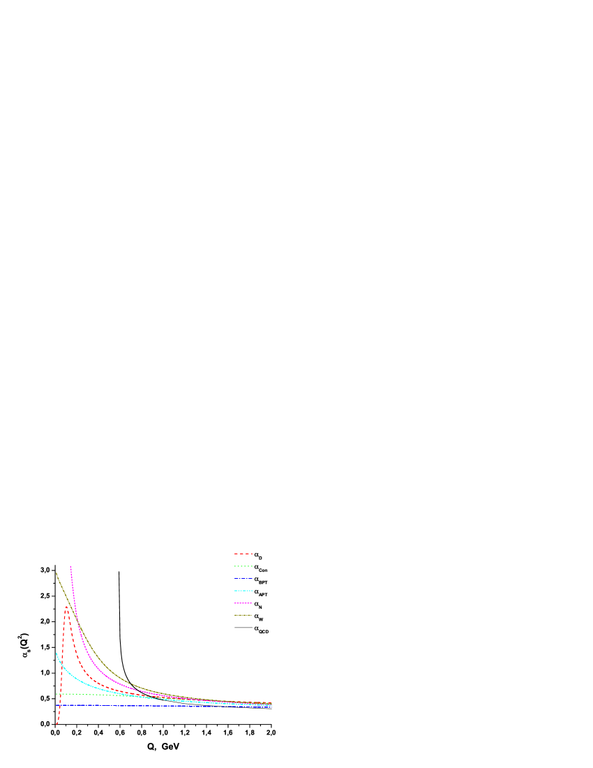
Figure 1: Various effective running strong coupling constants (see Eqs. (1), (7), (12), (18), (13) (15), (20))

Thus, there is a multitude of models for the running coupling constant as with a varying proportion between phenomenological and theoretical motivations. That is why one of the primary goals in this direction is to develop and improve methods that allow us to determine the QCD constant behavior.

Experimental determinations of $\alpha_{s}$ were regularly summarised and reviewed in [30, 31, 2]. These reviews provide information on modern methods of obtaining values of the constants from experimental data.

There are several techniques used to predict $\alpha_{s}$ at small $Q^{2}$, e.g. the bound state approach which reproduces hadronic characteristics and spectroscopy [5, 25, 32, 33], lattice QCD [34, 35], solving the Schwinger-Dyson equations [4, 36, 14, 17, 37], pich technique [38] and others. Matching the results of theoretical calculations with experimental data should lead to certain restrictions being put on the behavior of the running constant, which is one of the model parameters.

In this work we to study the IR behavior of the constant using combined approach, based on model calculations of meson characteristics (bound state approach) and current computing of pQCD corrections $\sim\nobreak\mathcal{O}\left(\alpha_{s}^{4}\right)$ to the sum rules of the nucleon [39, 40]. In this paper, we develop the approach of Ref. [41], which allows us to investigate the possible behavior of QCD constant in the infrared region.

To describe the properties of mesons we use Poincaré-covariant quark model based on the principles of relativistic Hamiltonian dynamics (RHD). The latter and their possible applications can be found in [42, 43, 44].

The basic requirement that restricts the possible behavior of $\alpha_{s}\left(Q^{2}\right)$ in this method is a matching condition between the model calculations and experimental values of the leptonic decay constants, masses of pseudoscalar and vector mesons and spin sum rules of nucleon.

The behavior of the modeling constant required to follow that of the standard one (1) for $Q>1\leavevmode\nobreak\ \mbox{\leavevmode\nobreak\ GeV}$ is considered an additional condition. Here, the behavior of the running constant is simulated using improved phenomenological parameterization (17) for different sets of $\alpha_{k},\gamma_{k}\;\left(k=1,\ldots,7\right)$. Using the phenomenological constant (17) significantly simplifies the solution of the two-particle equation (27). Instead of solving the equation (27) with different potentials, which differ in the behavior of QCD constants, we solve one equation with different sets of parameters $\alpha_{k}$ and $\gamma_{k}$ (see Eq.(28)).

The layout of the paper is as follows. Section 2 contains information on the modeling of QCD constant behavior with improved parameterization (17). A set of parameters that simulate the behavior of $\alpha_{s}(Q^{2})$ in the nonperturbative region is obtained.

In Sec. 3–4 Poincaré-covariant quark model of mesons and calculation of model leptonic meson decay constants are briefly described.

Sec. 5–6 is devoted to the strategy for extracting “optimal” behavior of $\alpha_{s}$ from the experimental data on leptonic constants and masses of mesons.

In Section 7–10 one can find an analysis of the experimental and theoretical information about the nucleon sum rules and the possible behavior of QCD constant in the infrared region, which follows from this data.

2 Modeling the effective coupling constant

To study infrared behavior of $\alpha_{s}$ one can try different shapes of the effective coupling or, equivalently, different ways to extrapolate the improved parameterization (17) for different sets of $\alpha_{k},\gamma_{k}\;\left(k=1,\ldots,7\right)$:

$$\alpha_{\mathrm{GI}}(Q^{2})=\sum_{k=1}^{n=7}\alpha_{k}\exp\left[-Q^{2}/\left(4\gamma^{2}_{k}\right)\right]\;$$ (21)

to the IR region of small $Q^{2}$. Further, to identify a specific set of parameters, we use the symbol $\texttt{N}_{\alpha}\;$.

This approach can be considered QCD constant model independent one, since we do not use any of the analytical expressions for the constants (1), (7), (12), (18), (13) (15), (20).

The behavior of the simulated constant required to follow that of the standard one (1) for $Q>1-2\mbox{\leavevmode\nobreak\ GeV}$ is considered a necessary condition (within errors).

The values of the QCD constant (1) and corresponding errors, which are used to calculate weighting coefficients, are obtained using RunDec program [45]. The number of points to fit is varied from 550 to 600 over the region of conformity (21) with the QCD constant. The region of $Q$ varies from $0.6$ to $200$ GeV.

Since the restriction put on the behavior of the running constant is based on the usage of a matching condition between experimental and simulated values of the characteristics of pseudoscalar and vector mesons, in which the constant is integrated out, this method will generally be “sensitive” to the square under the curve, which shows as behavior.

For this reason it is unnecessary to use a function of type (1); it is enough to get away with its approximation (21), which must reproduce the well studied $Q>1.0\mbox{\leavevmode\nobreak\ GeV}$ region.

We obtained sets of parameters differing in $\alpha_{\rm{crit.}}$ and the moment of the coupling (integral value):

$${A}\left(\mu\right)=\frac{1}{\mu}\int\limits^{\mu}_{0}\mathrm{d}\mathrm{k}\;\frac{\alpha_{s}\left(\mathrm{k}\right)}{\pi}\;$$ (22)

for $\mu=2\leavevmode\nobreak\ \mbox{\leavevmode\nobreak\ GeV}$,estimate of which was carried out in [16, 46] (Tables 1, 2).

Infrared behavior of the effective coupling constants can be divided into two types: a) constant freezing with a smooth and monotonic increase [4, 5, 8, 6, 25, 10] and b) modes with the maximum, when $\alpha_{s}\to 0$ for $Q^{2}\to 0$ [47, 18, 19, 14, 15].

Therefore, we simulated both types of behavior: the first one includes “freezing” the running coupling constant starting from some value $Q_{0}=0.6\div 1.0$ (see Table 1), while the second regime emulates the behavior with a peak in the nonperturbative region (see Table 2).

Table 1: Sets of constants (21) with various $\alpha_{\mathrm{crit.}}$ for “freezing” regimes (see left panel of Fig.  2) .

$\texttt{N}_{\alpha}$, (number of set)	$\alpha_{\rm crit.}$	${A}\left(2\leavevmode\nobreak\ \mbox{GeV}\right)$
1-a	$4.635\pm 0.006$	$0.391\pm 0.003$
2-a	$3.230\pm 0.007$	$0.318\pm 0.003$
3-a	$1.300\pm 0.003$	$0.202\pm 0.001$
4-a	$1.087\pm 0.003$	$0.186\pm 0.001$
5-a	$0.844\pm 0.003$	$0.168\pm 0.001$
6-a	$0.687\pm 0.006$	$0.155\pm 0.002$
7-a	$0.660\pm 0.007$	$0.151\pm 0.002$

Table 2: Sets of constants (21) with various $\alpha_{\mathrm{crit.}}$ for regimes with a peak in the nonperturbative region (see right panel of Fig.  2).

$\texttt{N}_{\alpha}$, (number of set)	$\bar{A}\left(2\leavevmode\nobreak\ \mbox{GeV}\right)$
1-b	$0.238\pm 0.014$
2-b	$0.192\pm 0.008$
3-b	$0.178\pm 0.016$
4-b	$0.165\pm 0.009$
5-b	$0.150\pm 0.005$
6-b	$0.134\pm 0.023$
7-b	$0.127\pm 0.015$

A comparative graph for the coupling constants fixed by Eq. (1) and various regimes of the effective constant behavior (21) is demonstrated in Fig. 2.

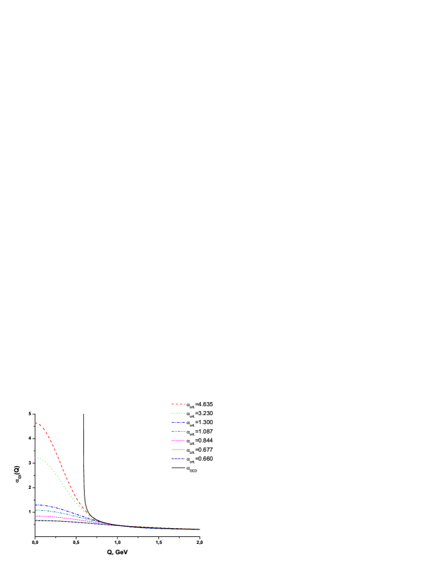
(a) Freezing regime.

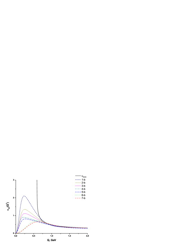
(b) Modes with a peak in the nonperturbative region.

Figure 2: Dependence of the running strong coupling constant for pQCD (1) and phenomenological parameterization (21).

3 Poincaré-covariant quark model of mesons

In our article we use the description of bound states with the help of relativistic Hamiltonian dynamics (RHD) that is the generalization of the ordinary quantum mechanics. [48, 43]. RHD is also dubbed Poincaré-invariant quantum mechanics (see, for instance, [44]).

The RHD differs from the ordinary non-relativistic quantum mechanics, as the main requirement for the operators of the complete set of states is the one that the generators that make up the operators should follow the algebra of Poincaré group.

In the framework of RHD, the interaction, which is determined by the generators of the Poincaré group $\hat{P}_{\mu}$ and $\hat{M}^{\mu\nu}$ is introduced as follows. The construction of generators for a system of interacting particles starts from the generators of an appropriate system composed out of noninteracting particles, and then interaction is added so that the obtained generators also satisfy the commutation relations of Poincaré group. We shall not focus ourselves on the details of RHD and it’s connection with quantum field theory and special relativity but we refer reader to the paper [43] and references therein.

Unlike the case of a usual non-relativistic quantum mechanics, in the relativistic case it is necessary to add interaction $\hat{V}$ in more than one generator to satisfy the algebra of the Poincaré group. Dirac [48] has shown that there is no unambiguous separation of generators into dynamic set (generators containing the interaction $\hat{V}$) and kinematic set. There are three versions of separation on dynamic and kinematic sets (so-called RHD forms): point form, instant form and dynamics on light front.

In all three forms the interaction contains mass operator $\hat{M}$ i.e. $\hat{M}\equiv M_{0}+\hat{V}$, where $M_{0}$ is an effective mass of a system of noninteracting particles with masses $m_{q}$ and $m_{Q}$:

$$M_{0}=\sqrt{m_{q}^{2}+{\bf k}^{2}}+\sqrt{m_{Q}^{2}+{\bf k}^{2}}\leavevmode\nobreak\ .$$ (23)

Here

$$\mathbf{k}\mathbf{=}\frac{1}{2}\left(\mathbf{p}_{1}-\mathbf{p}_{2}\right)+\frac{\mathbf{P}}{\widetilde{M}_{0}\left(\omega_{\widetilde{M}_{0}}\left(\mathrm{P}\right)+\widetilde{M}_{0}\right)}\times$$

$$\times\left(m_{Q}^{2}-m^{2}_{q}-\widetilde{M}_{0}\left[\omega_{m_{Q}}\left(\mathrm{p}_{2}\right)-\omega_{m_{q}}\left(\mathrm{p}_{1}\right)\right]\right)$$ (24)

is the relative momentum and $\mathbf{P}$ is the total momentum of the free-system

$$\mathbf{P}=\mathbf{p_{1}+p_{2}}\;,$$ (25)

$$\widetilde{M}_{0}=\sqrt{\left[\omega_{m_{Q}}\left(\mathrm{p}_{2}\right)+\omega_{m_{q}}\left(\mathrm{p}_{1}\right)\right]^{2}-\mathbf{P}^{2}}$$

and $\omega_{m}\left(\mathrm{p}\right)=\sqrt{m^{2}+{\bf p}^{2}}$, $\mathrm{k}=\left|\mathbf{k}\right|$.

In the framework of RHD the bound system with momentum $\mathbf{Q}$, eigenvalues $M$, spin $J$ and it’s projection $\mu$ is described by the wave function $\Phi^{J\mu}_{\mathbf{Q};\;\sigma_{1}\sigma_{2}}\left({\bf k}\right)$ of two-particle state, which satisfies the equation [43]

$$\sum_{\lambda_{1},\lambda_{2}}\int<{\bf k},\sigma_{1},\sigma_{2}\parallel\hat{V}\parallel\ {\bf k}^{\prime},\lambda_{1},\lambda_{2}>\times$$

$$\times\Phi^{J\mu}_{\mathbf{Q};\lambda_{1}\lambda_{2}}\left({\bf k}^{\prime}\right)\mathrm{d}{\bf k}^{\prime}=\left(M-M_{0}\right)\Phi^{J\mu}_{\mathbf{Q};\sigma_{1}\sigma_{2}}\left({\bf k}\right)\;.$$ (26)

The radial equation for two-particle bound state in the center-momentum system ($\mathbf{Q}=0$) has the following form

$$\sum_{\ell^{\prime},S^{\prime}}\int\limits_{0}^{\infty}V^{J}_{\ell,S\;;\ell^{\prime},S^{\prime}}\left(\mathrm{k},\mathrm{k^{\prime}}\right)\Phi^{J\mu}_{\ell^{\prime},S^{\prime}}\left(\mathrm{{k}^{\prime}}\right){\mathrm{{k}^{\prime}}}^{2}\mathrm{d}{\mathrm{k}}^{\prime}=\left(M-M_{0}\right)\Phi^{J\mu}_{\ell,S}\left(\mathrm{{k}}\right)\;.$$ (27)

To describe specific bound systems, it is necessary to determine the interaction potential between particles. It should be noted that different potentials can be used to describe a bound system of the same composition. Such a selection of potentials automatically distinguishes different Poincaré-covariant models.

In our case the interquark potential in coordinate representation from [5] is used, which is considered a sum of Coulomb, linear confinement, and spin-spin parts for pseudoscalar and vector mesons:

$$\hat{V}\left(\mathrm{r}\right)=\hat{V}_{Coulomb}(\mathrm{r})+\hat{V}_{linear}(\mathrm{r})+\hat{V}_{{S}{S}}(\mathrm{r})\;,$$ (28)

$$\hat{V}_{Coulomb}(\mathrm{r})=-\frac{4}{3}\;\frac{\alpha_{s}\left(\mathrm{r}\right)}{\mathrm{r}}=-\frac{4}{3\;\mathrm{r}}\;\sum_{k=1}^{7}\alpha_{k}\,\hbox{erf}(\tau_{k}\,\mathrm{r})\;,$$

$$\hat{V}_{linear}(\mathrm{r})=\sigma\;\mathrm{r}\left[\frac{\exp(-b^{2}\mathrm{r}^{2})}{\sqrt{\pi}\;b\;\mathrm{r}}+\left(1+\frac{1}{2\;b^{2}\mathrm{r}^{2}}\right)\;\hbox{erf}(b\;\mathrm{r})\right]+w_{0}\;,$$

$$\hat{V}_{{S}{S}}(\mathrm{r})=-\frac{32\;\left({\mathbf{S}}_{q}{\mathbf{S}}_{Q}\right)}{9\sqrt{\pi}\;m_{q}\;m_{Q}}\sum_{k=1}^{7}\alpha_{k}\;\tau_{k}^{3}\;\exp(-\tau_{k}^{2}\mathrm{r}^{2})\;,$$

where parameter $\tau_{k}$ is deduced from the relation ${1/\tau_{k}^{2}}={1/\gamma_{k}^{2}}+{1/\mathrm{b}^{2}}$, $\hbox{erf}(x)$) is an error function, and $\mathbf{S}_{q,\;Q}$ denote quark spin operators.

To derive the potential (28) given in, the procedure of “smearing” was applied according to the following rule [5]:

$$\tilde{f}\left(\mathbf{r}\right)=\int\mathrm{d}\mathbf{r}^{\prime}\rho\left(\mathbf{r}-\mathbf{r}^{\prime}\right)f\left(\mathbf{r}^{\prime}\right)\;,$$

where the “smearing” function with parameter $\mathrm{b}$ is chosen in the form

$$\rho\left(\mathbf{r}-\mathbf{r}^{\prime}\right)=\frac{\mathrm{b}^{3}}{\pi^{3/2}}\exp\left[-\mathrm{b}\left(\mathbf{r}-\mathbf{r}^{\prime}\right)^{2}\right]\;.$$

4 Leptonic meson decay constants in Poincaré-covariant model

Upon the removal of element $V_{Qq}$ of the Cabibbo-Kobayashi-Maskawa matrix, the constant $f_{P}$ of the leptonic decay $f_{P}$$P(Q\bar{q})\to\ell+\nu_{\ell}$ for a pseudoscalar meson $P(Q\bar{q})$ is defined by the relation:

$$j^{\mu}_{P}\equiv\left<0\left|\hat{J}^{\mu}_{A}\left(0\right)\right|{\bf P},M_{P}\right>_{in}=\mathrm{i}\left(1/2\pi\right)^{3/2}\frac{P^{\mu}f_{P}}{\sqrt{2\;\omega_{M_{P}}\left({\mathrm{P}}\right)}}\;,$$ (29)

where the electroweak axial current $\hat{J}^{\mu}_{A}(0)$ and the vector of a meson state with mass $M_{P}$ are taken in the Heisenberg representation. Vectors of states in this expression are normalized as follows: $\left<\mathbf{P},M_{P}\right.\left|\mathbf{P}^{\prime},M_{P}\right>$=$\delta(\mathbf{P}-\mathbf{P}^{\prime})$.

The decay width for $P(Q\bar{q})\to\ell+\nu_{\ell}$ is given by the expression

$$\Gamma_{P}=\frac{G_{F}^{2}\left|V_{Qq}\right|^{2}}{8\pi}m_{\ell}^{2}M_{P}f_{P}^{2}\left(1-\frac{m_{\ell}^{2}}{M_{P}^{2}}\right)^{2}\;,$$ (30)

where $m_{\ell}$ is lepton mass and $G_{F}$ is a Fermi constant.

In the case of leptonic decays of vector mesons $V(Q\bar{q})\to\ell+\bar{\ell}$ relations analogous to the expressions given in (29) and (30) will take the form

$$j^{\mu}_{V}\equiv\left<0\left|\hat{J}^{\mu}_{V}\left(0\right)\right|{\bf P},M_{V},\lambda\right>_{in}=\mathrm{i}\left(1/2\pi\right)^{3/2}\frac{\varepsilon^{\mu}_{\lambda}M_{V}f_{V}}{\sqrt{2\;\omega_{M_{V}}\left({\mathrm{P}}\right)}}$$

with $\varepsilon^{\mu}_{\lambda}$ being the polarization vector of a vector meson with mass $M_{V}$. Respectively, the decay width for $V(Q\bar{q})\to\ell+\bar{\ell}$ is given by the following expression:

$$\Gamma_{V}=\frac{4\pi\alpha^{2}}{3\;M_{V}}f_{V}^{2}\left(1+\frac{2\;m_{\ell}^{2}}{M_{V}^{2}}\right)\sqrt{1-\frac{4\;m_{\ell}^{2}}{M_{V}^{2}}}\;,$$ (31)

where $\alpha$ stands for the fine structure constant. In [49, 50] coinciding integral representations for the constants of leptonic pseudoscalar $f_{P}$ and vector $f_{V}$, meson decays are obtained within the framework of Poincaré-covariant models based on the point and instant forms of RHD:

$$f_{P}\left(m_{q},m_{Q}\right)=\frac{N_{c}}{\pi\sqrt{2}}\int\limits_{0}^{\infty}\mathrm{d}\mathrm{k}\hskip 2.0pt\mathrm{k}^{2}\psi^{P}\left(\mathrm{k}\right)\sqrt{\frac{M_{0}^{2}-(m_{q}-m_{Q})^{2}}{\omega_{m_{q}}\left(\mathrm{k}\right)\omega_{m_{Q}}\left(\mathrm{k}\right)}}\frac{\left(m_{q}+m_{Q}\right)}{M_{0}^{3/2}}\;,$$ (32)

$$f_{V}\left(m_{q},m_{Q}\right)=\frac{N_{c}}{\sqrt{2}\pi}\int\limits_{0}^{\infty}\mathrm{d}\mathrm{k}\hskip 2.0pt\mathrm{k}^{2}\psi^{V}\left(\mathrm{k}\right)\frac{\sqrt{\left(\omega_{m_{q}}\left(\mathrm{k}\right)+m_{q}\right)\left(\omega_{m_{Q}}\left(\mathrm{k}\right)+m_{Q}\right)}}{\sqrt{\omega_{m_{q}}\left(\mathrm{k}\right)+\omega_{m_{Q}}\left(\mathrm{k}\right)}\;\omega_{m_{q}}\left(\mathrm{k}\right)\omega_{m_{Q}}\left(\mathrm{k}\right)}\times$$

$$\times\left(1+\frac{\mathrm{k}^{2}}{3\left(\omega_{m_{q}}\left(\mathrm{k}\right)+m_{q}\right)\left(\omega_{m_{Q}}\left(\mathrm{k}\right)+m_{Q}\right)}\right)\;,$$ (33)

where $N_{c}$ is a number of quark colors.

Analogous integral representation for $f_{P}$ is derived in [51] in the context of the Poincaré-covariant model based on the light front dynamics. The representations in (32) and (33) in the nonrelativistic case become classical expressions in which constants are directly proportional to the meson wave function in the position representation at the origin $\mathrm{r}=0$.

5 Selection of model parameters

Let us solve the eigenvalue problem (27) with potential (28) by using variational method with oscillator and Coulomb (for $B$-mesons) wave functions. In this method it is required to minimize the functional

$$M\left(m_{q},m_{Q},\beta,w_{0},b,\sigma\right)=\langle\psi\left(\beta\right)|{\hat{M}}|\psi\left(\beta\right)\rangle=\langle\psi|\hat{M}_{0}|\psi\rangle+\langle\psi|\hat{V}|\psi\rangle\;,$$

where $\psi\left(\beta\right)$ is a trial wave function.

The potential of the model (28) has the following free parameters: gluon string tension $\sigma$, smearing factor $\mathrm{b}$, and $w_{0}$. Quark masses $m_{q,Q}$ and sets of constants $\alpha_{k},\gamma_{k}$, which characterize the behavior of the effective strong coupling constant, are also considered as parameters. Note that the values of parameters $\beta,w_{0},\sigma$ depend on the quark flavors.

Let’s consider a procedure for fixing the numeric values of the potential parameters. The parameter of the potential’s linear part lies within the range of $0.18$ to $0.20$ $\mbox{GeV}^{2}$ [5, 52, 53, 27] in a large number of models. Therefore, we assume in the calculations that

$$\sigma=\bar{\sigma}\pm\Delta\sigma\;=\;\left(0{.}19\pm 0.01\right)\;\;\mbox{GeV}^{2}\;.$$ (34)

Wave function parameter $\beta$ and all other potential parameters are determined by solving the following system of equations:

$$\frac{\partial M_{P,V}\left(\beta,\sigma\right)}{\partial\beta}\left.\right.\bigg{|}_{\beta_{min},\tilde{\sigma}}=0\leavevmode\nobreak\ \;,\;\;M_{P}\left(w_{0},\beta_{min},\tilde{\sigma}\right)=M_{P}\pm\Delta M_{P}\;,$$ (35)

$$M^{S=1}_{V}\left(\beta,\sigma\right)-M^{S=0}_{P}\left(\beta,\sigma\right)\left.\right|_{\beta_{min},\tilde{\sigma}}=M_{V}-M_{P}\pm\delta M_{\rm{vp}}\;,$$ (36)

$$f_{P}\left(m_{q},m_{Q},\beta_{min}\right)=f_{\rm{exp}}^{P}\pm\Delta f_{\rm{exp}}^{P}\;,$$ (37)

$$f_{V}\left(m_{q},m_{Q},\beta_{min}\right)=f_{\rm{exp}}^{V}\pm\Delta f_{\rm{exp}}^{V}\;,$$ (38)

where Eqs. (35) and (36) are minimum condition and requirement for simulated values of meson masses to match their experimental counterparts. Quantities $M_{P,V}$ are experimental values of pseudoscalar and vector meson masses and $\Delta M_{P,V}$ are their experimental measurement errors. The last two equations mean that the values of leptonic coupling constants for pseudoscalar and vector mesons, obtained using the Poincaré-covariant model coincide (see (32), (33)) with experimental values $f_{\rm{exp}}$ within the errors.

5.1 Masses of $u,d$ and $s$ quarks

Assuming that constituent masses of u and d quarks are approximately equal [5]:

$$m_{d}-m_{u}\equiv\Delta m_{ud}=\left(4\pm 1\right)\mbox{MeV}\;,$$ (39)

we obtain a system of equations from (35)–(38):

$$\left\{\begin{array}[]{l}f_{V}\left(m_{u},m_{d},\beta\right)=f_{\rm{exp}}^{\rho^{0}}\pm\Delta f_{\rm{exp}}^{\rho^{0}}\;,\\ f_{P}\left(m_{u},m_{d},\beta\right)=f_{\rm{exp}}^{\pi^{\pm}}\pm\Delta f_{\rm{exp}}^{\pi^{\pm}}\;.\\ \end{array}\right.$$

Using experimental data for $\pi^{\pm}$ and $\rho^{0}$ mesons [54]

$$f_{\pi^{\pm}}^{P}=\left(130.41\pm 0.03\pm 0.20\right)\leavevmode\nobreak\ \mbox{MeV}\;,\;\;f_{\rho^{0}}^{V}=\left(156.2\pm 1.2\right)\leavevmode\nobreak\ \mbox{MeV}\;,$$

where the last numerical value is obtained from (31) and the experimental data of width $\Gamma_{\rho^{0}}=7.02\pm 0.11\mbox{\leavevmode\nobreak\ \leavevmode\nobreak\ keV}$ for the decay $\rho^{0}\to e^{+}e^{-}$ [55], we obtain the values of $u$- and $d$-quark masses:

$$m_{u}=\left(239.8\pm 2.3\right)\mbox{MeV}\;\;,\;\;m_{d}=\left(243.8\pm 2.3\right)\mbox{MeV}\;.$$ (40)

Depending on the behavior of the running strong coupling constant $\alpha_{s}\left(Q^{2}\right)$, the solution of equations system

$$\left\{\begin{array}[]{l}\partial M_{V}\left(\beta,\ldots\right)/\partial\beta=0\leavevmode\nobreak\ \;,\;\;M_{K^{+}}\left(\beta,\ldots\right)=M_{K^{\pm}}\pm\Delta M_{K^{\pm}}\;,\\ M^{S=1}_{V}\left(\beta,\ldots\right)-M^{S=0}_{P}\left(\beta,\ldots\right)=M_{K^{*}}-M_{K^{\pm}}\pm\delta M_{K^{*}-K^{\pm}}\;,\\ f_{P}\left(m_{u},m_{s},\beta\right)=f_{\rm{exp}}^{K^{\pm}}\pm\Delta f_{\rm{exp}}^{K^{\pm}}\;.\\ \end{array}\right.$$ (41)

with account for the experimental data [55]

$$M_{K^{+}}=\left(493.677\pm 0.016\right)\leavevmode\nobreak\ \mbox{MeV}\;,\;\;f_{K^{\pm}}^{P}=\left(156.1\pm 0.2\pm 0.8\pm 0.2\right)\leavevmode\nobreak\ \mbox{MeV}\;,$$

$$\Delta M_{\mathrm{exp}}=M_{K^{*}}-M_{K^{\pm}}=\left(397.983\leavevmode\nobreak\ \pm 0.261\right)\mbox{\leavevmode\nobreak\ \leavevmode\nobreak\ MeV}\;$$

and the value of $u$-quark mass (40) gives the results presented in Table 3 with experimental and theoretical uncertainties indicated.

Table 3: Allowed values of $s$–quark mass for different regimes $\texttt{N}_{\alpha}$ of $\alpha_{s}$-behavior (with various $\alpha_{\mathrm{crit.}}$ and ${A}\left(\mu\right)$ (22)).

$\texttt{N}_{\alpha}$	$\alpha_{\rm crit.}$	$m_{s}\;,\mbox{\leavevmode\nobreak\ MeV}$	$\texttt{N}_{\alpha}$	$m_{s}\;,\mbox{\leavevmode\nobreak\ MeV}$
1-a	$4.635\pm 0.006$	$478.4\pm 23.1$	1-b	$467.2\pm 28.9$
2-a	$3.230\pm 0.007$	$469.1\pm 23.5$	2-b	$461.6\pm 28.7$
3-a	$1.300\pm 0.003$	$460.4\pm 25.0$	3-b	$461.5\pm 31.1$
4-a	$1.087\pm 0.003$	$461.0\pm 25.6$	4-b	$463.0\pm 30.6$
5-a	$0.844\pm 0.003$	$463.3\pm 26.7$	5-b	$460.9\pm 29.9$
6-a	$0.687\pm 0.006$	$466.5\pm 28.0$	6-b	$471.1\pm 29.9$
7-a	$0.660\pm 0.007$	$466.6\pm 28.0$	7-b	$473.2\pm 30.7$

5.2 Masses of $c$ and $b$ quarks

To calculate leptonic constants for heavy mesons we need to know the masses of $c$ and $b$ quarks. In order to compute the constraints on the values of quarks the data on $c\bar{c}$ ($\eta_{c}$ and $J/\psi$ mesons) and $b\bar{b}$ ($\eta_{b}$ and $\gamma\left(1S\right)$ mesons) systems are used:

$$M_{\eta}=\left(2981.0\pm 1.1\right)\leavevmode\nobreak\ \mbox{MeV}\;,\;\;M_{J/\psi}=\left(3096.916\pm 0.011\right)\leavevmode\nobreak\ \mbox{MeV}\;,$$

$$M_{\eta_{b}}=\left(9391.0\pm 2.8\right)\leavevmode\nobreak\ \mbox{MeV}\;,M_{\gamma\left(1S\right)}=\left(9460.30\pm 0.26\right)\leavevmode\nobreak\ \mbox{MeV}\;.$$ (42)

Since these systems consist of particles with equal masses, it is enough to use experimental data only for leptonic decays of vector states in order to fix the masses of the quarks:

$$f_{\gamma\left(1S\right)}^{V}=\left(238.4\pm 1.6\right)\leavevmode\nobreak\ \mbox{MeV}\;,\;\;f_{J/\psi}^{V}=\left(277.6\pm 4\right)\leavevmode\nobreak\ \mbox{MeV}\;.$$ (43)

A solution to the system of equations analogous to Eqs. (41) leads to constraints on the masses of $c$ and $b$ quarks that are presented in Table  4.

Table 4: Allowed values of $c$ and $b$ quarks masses for different regimes $\texttt{N}_{\alpha}$ of the $\alpha_{s}$-behavior (with various $\alpha_{\mathrm{crit.}}$ and ${A}\left(\mu\right)$ (22)).

$\texttt{N}_{\alpha}$	$m_{c}\;,\mbox{\leavevmode\nobreak\ GeV}$	$m_{b}\;,\mbox{\leavevmode\nobreak\ GeV}$	$\texttt{N}_{\alpha}$	$m_{c}\;,\mbox{\leavevmode\nobreak\ GeV}$	$m_{b}\;,\mbox{\leavevmode\nobreak\ GeV}$
1-a	$1.500\pm 0.068$	$3.668\pm 0.158$	1-b	$1.454\pm 0.080$	$3.814\pm 0.121$
2-a	$1.473\pm 0.069$	$3.748\pm 0.159$	2-b	$1.420\pm 0.077$	$3.919\pm 0.130$
3-a	$1.410\pm 0.068$	$3.965\pm 0.174$	3-b	$1.410\pm 0.091$	$3.746\pm 0.258$
4-a	$1.399\pm 0.069$	$3.995\pm 0.174$	4-b	$1.396\pm 0.082$	$3.965\pm 0.126$
5-a	$1.385\pm 0.069$	$4.029\pm 0.178$	5-b	$1.372\pm 0.074$	$4.281\pm 0.228$
6-a	$1.373\pm 0.071$	$4.057\pm 0.157$	6-b	$1.382\pm 0.100$	$4.034\pm 0.059$
7-a	$1.366\pm 0.070$	$4.092\pm 0.180$	7-b	$1.373\pm 0.091$	$4.066\pm 0.090$

6 Determination of the “optimal” $\texttt{N}_{\alpha}$

Optimal value for $\alpha_{\rm{crit.}}$ and, respectively, a possible regime of $\alpha_{s}\left(Q^{2}\right)$ behavior will be chosen by using the experimental data on the constants of leptonic decays of pseudoscalar heavy mesons ($D$ and $D_{s}$ mesons).

The quantity $\chi^{2}$ will be the main criterion used in this selection procedure. To this end, let us compute the $\chi^{2}$ quantity

$$\chi^{2}\left(\texttt{N}_{\alpha}\right)=\sum_{i=1}^{k}\frac{\left(f^{P}_{i,\;\mathrm{exp}}-f^{P}_{i}\left(m_{q},m_{Q},\beta\right)\right)^{2}}{\left(\delta f^{P}_{i,\;\mathrm{exp}}\right)^{2}+\left(\delta f^{P}_{i,\;\mathrm{teor}}\right)^{2}}$$ (44)

for various regimes of strong coupling constant behavior and find its minimum. The quantity $\delta f^{P}_{\mathrm{teor}}$ includes all uncertainties related with both theoretical (originating from calculations) and experimental errors for meson masses whose values served as benchmarks for finding model parameters. In the asymptotic limit, the quantity $\chi^{2}\left(\texttt{N}_{\alpha}\right)$ will be distributed like $\chi^{2}$ with $k$ degrees of freedom.

Using the following experimental values from [54]

$$f_{D,\mathrm{exp}}^{P}=(206.7\pm 8.9)\leavevmode\nobreak\ \mbox{MeV}\;,\;f_{D_{s},\mathrm{exp}}^{P}=(260.0\pm 5.4)\leavevmode\nobreak\ \mbox{MeV}$$

and calculations of the leptonic constants for pseudoscalar mesons within a framework of the Poincaré-covariant model, we find the dependence of $\chi^{2}\left(\texttt{N}_{\alpha}\right)$ has on the regimes of $\alpha_{s}$ behavior. These results we presented in Table 5, along with the acceptance probabilities $P$ (in $\%$).

Table 5: The values of $\chi^{2}\left(\texttt{N}_{\alpha}\right)$ (44) and acceptance probabilities $P$ of model for various regimes of $\alpha_{s}$ behavior.

$\texttt{N}_{\alpha}$	$\chi^{2}\left(\texttt{N}_{\alpha}\right)$	$P,\;\%$	$\texttt{N}_{\alpha}$	$\chi^{2}\left(\texttt{N}_{\alpha}\right)$	$P,\;\%$
1-a	$6.74$	$3.4$	1-b	$3.07$	$21.5$
2-a	$4.63$	$9.9$	2-b	$1.51$	$46.9$
3-a	$1.33$	$51.3$	3-b	$0.77$	$68.1$
4-a	$0.84$	$65.8$	4-b	$0.39$	$82.1$
5-a	$0.32$	$85.0$	5-b	$0.34$	$84.2$
6-a	$0.08$	$96.1$	6-b	$0.06$	$97.2$
7-a	$0.05$	$97.6$	7-b	$0.02$	$99.0$

As follows from the calculations (see, Table 5) models with freezing constant $\texttt{N}_{\alpha}=\nobreak\texttt{6-{a}},\texttt{7-{a}}$ have a minimum of $\chi^{2}$ and the maximum acceptance probability $P>95\;\%$ . The highest acceptance probability ($P>95\;\%$) for modes with a peak are constants for the sets $\texttt{N}_{\alpha}=\texttt{6-{b}}$ and $\texttt{N}_{\alpha}=\texttt{7-{b}}$.

Model leptonic constants of $D$ and $D_{s}$ mesons for $\texttt{N}_{\alpha}=\texttt{7-{a}}$ are

$$f_{D}^{P}=(204.6\pm 4.5)\leavevmode\nobreak\ \mbox{MeV}\;,\;f_{D_{s}}^{P}=(259.3\pm 10.4)\leavevmode\nobreak\ \mbox{MeV}\;.$$

Values (6) are in good agreement with the data (6).

However, it should be noted that models 5-a, 6-a, and 4-b, 5-b, as well as 6-b have relatively larger probabilities and cannot be definitely discarded since their $\chi^{2}/2\leq 1$. For further restrictions additional information is needed. The data on $B$-meson decays can provide such information.

At present, from our point of view, there is a considerable variation in determining the leptonic constant of a charged $B$ meson. An experimental value of the quantity (see [56, 57, 58, 59, 60])

$$f_{B}^{P}\left|V_{ub}\right|=\left(7.2\div 10.1\right)\times 10^{-1}\leavevmode\nobreak\ \mbox{MeV}\;,$$

with a modern constraint imposed on $\left|V_{ub}\right|=\left(4.15\pm 0.49\right)\times 10^{-3}$ [61] entails substantial variation in $f_{B}^{P}$:

$$f_{B}^{P}=\left(208.4\pm 42.7\right)\leavevmode\nobreak\ \mbox{MeV}\;.$$

There also is a considerable variation in theoretical predictions for the leptonic decay constants of ${B}^{\pm}$-mesons: from $f_{B}^{P}=\left(147^{+34}_{-38}\right)\leavevmode\nobreak\ \mbox{MeV}$ in [62] to $f_{B}^{P}=\nobreak\left(230\pm 23\right)\leavevmode\nobreak\ \mbox{MeV}$ in [63].

In our approach, for the optimal regime with freezing constant 7-a, the leptonic decay constant is found to be

$$f_{B}^{P}=\left(226.2\pm 3.9\right)\leavevmode\nobreak\ \mbox{MeV}\;,$$ (45)

while for the regime with a peak 7-b we have

$$f_{B}^{P}=\left(216.7\pm 5.8\right)\leavevmode\nobreak\ \mbox{MeV}\;,$$ (46)

The value in (46) is in good agreement with the data of theoretical SM prediction [64]:

$$f_{B}^{P}=\left(216.0\pm 22.0\right)\leavevmode\nobreak\ \mbox{MeV}\;,$$

but it is far enough from the data of BaBar and Belle collaborations [58, 60, 56], whose values lie within the range $f_{B,\mathrm{exp}}^{P}=\left(246.8\pm 45.6\right)\leavevmode\nobreak\ \mbox{MeV}$. Value (45) is closer to the BaBar and Belle data.

Thus, on the base of existing uncertainties and experimental data on the leptonic constants of heavy mesons, one can suppose that $\alpha_{s}$- constant behavior has to freezing modes with $\texttt{N}_{\alpha}=\texttt{5-{a}}-\texttt{7-{a}}$ and $\alpha_{\mathrm{crit.}}=(0.660\div 0.844)$ as well as those with 6-b, 7-b (can not definitely exclude the behavior $\texttt{N}_{\alpha}=\texttt{4-\rm{a}}$, where $\alpha_{\mathrm{crit.}}=1.087$ and modes 3-b–5-b).

Note that bound state approach does not allow for the unique identification of $\alpha_{s}$ behavior, since the parameter ${A}\left(\mu\right)$, which this method is sensitive to, is related with the latter indirectly through integration over the momentum transfer $Q$.

Indeed, as follows from Tables 1 and 2, the values of ${A}\left(\mu\right)$ for qualitatively different regimes with freezing and peak are close to each other and lie within the range of 0.13-0.19. These values of ${A}\left(\mu\right)=0.13-0.19$ are quite consistent with the experimental data from [46]: ${A}_{\mathrm{fit}}\left(\mu\right)=0.16\pm 0.01(\mathrm{exp})\pm 0.02(\mathrm{th})$.

To clarify the behavior of the effective coupling constant one needs to analyze the experimental results from SLAC [65, 66] and JLab [67, 68, 69, 70, 71] on the first moments of spin structure functions $g^{p,n}_{1}(x,Q^{2})$.

7 First moments of spin structure functions

The first moments of spin-dependent proton and neutron structure functions $g_{1}^{p,n}\left(x,Q^{2}\right)$ are defined as

$$\Gamma^{p,n}_{1}(Q^{2})=\int\limits_{0}^{1}g_{1}^{p,n}\left(x,Q^{2}\right)\mathrm{d}x\;.$$ (47)

The pQCD result (47) (in the $\overline{\mathrm{MS}}$-scheme) is

$$\Gamma^{p,n}_{1}(Q^{2})=\left\{\frac{1}{12}\left(\pm g_{A}+\frac{a_{8}}{3}\right)C_{NS}\left(Q^{2}\right)+\frac{{a}_{0}^{inv}}{9}C_{SI}^{inv}\left(Q^{2}\right)\right\}+\Delta_{\mathrm{HT}}^{p,n}(Q^{2})\;,$$ (48)

where $C_{NS}\left(Q^{2}\right)$ and $C_{SI}^{inv}\left(Q^{2}\right)$ are the first moments of the non-singlet and singlet Wilson coefficient functions, respectively. Here the $+(-)$ sign of the $g_{A}$ term holds for the proton (neutron).

The coefficients $C_{NS}$ and $C_{S}^{inv}$ have been calculated in perturbative QCD (in the $\overline{\mathrm{MS}}$ scheme) up to the third and fourth order in $\alpha_{s}$ (see [72, 73, 74, 39])

$$C_{NS}\left(Q^{2}\right)=1+\sum\limits_{k=1}^{4}d^{NS}_{k}a_{s}^{k}(Q^{2})\;,$$ (49)

$$C_{SI}^{inv}\left(Q^{2}\right)=1+\sum\limits_{k=1}^{3}d^{SI}_{k}a_{s}^{k}(Q^{2})\;,$$ (50)

where

$$a_{s}(Q^{2}) = \alpha_{s}(Q^{2})/\pi\;,$$

$$d_{1}^{NS} = -1\;,$$

$$d_{2}^{NS} = -4.583+0.333\,n_{f}\;,$$

$$d_{3}^{NS} = -41.44+7.607\,n_{f}-0.1775\,n_{f}^{2}\;,$$

$$d_{4}^{NS} = -479.4475+123.3914\,n_{f}-7.6975\,n_{f}^{2}+0.10374\,n_{f}^{3}\;,$$ (51)

and

$$d_{1}^{SI} = \frac{1}{4\beta_{0}}\left(-11+\frac{8}{3}\,n_{f}\right)\;,$$

$$d_{2}^{SI} = \frac{1}{4^{2}\beta_{0}^{2}}\left(-554.583+214.466\,n_{f}-16.4757\,n_{f}^{2}+0.5537\,n_{f}^{3}\right)\;,$$

$$d_{3}^{SI} = \frac{1}{4^{3}\beta_{0}^{3}}\left(-55156.5+29692.9\,n_{f}-5292.89\,n_{f}^{2}+434.2\,n_{f}^{3}-\right.$$ (52)

$$- \left.16.139\,n_{f}^{4}+0.229263\,n_{f}^{5}\right)\;.$$

Constants $g_{A}=1.2701\pm 0.0025$ [55] and $a_{8}=0.585\pm 0.025$ [75] are the isovector and $SU(3)$ octet axial charges, respectively. The ${a}_{0}^{inv}$ is the renormalization group invariant (i.e. $Q^{2}$ independent) [72, 74].

The $Q^{2}$ evolution of the axial singlet charge $a_{0}(Q^{2})$ [73, 74] for $n_{f}=3$ quarks flavors is

$$a_{0}(Q^{2}) = {a}_{0}^{inv}\exp\left(\int\limits^{a_{s}}\frac{\gamma SI(x)}{\beta(x)}\mathrm{d}x\right)\approx$$ (53)

$$\approx \left(1+\frac{2}{3}a_{s}(Q^{2})+\frac{131}{108}a_{s}^{2}(Q^{2})+\frac{41477}{11664}a_{s}^{3}(Q^{2})\right){a}_{0}^{inv}\;.$$

The product ${a}_{0}^{inv}C_{SI}^{inv}\left(Q^{2}\right)$ is often rewritten in the form

$${a}_{0}^{inv}C_{SI}^{inv}\left(Q^{2}\right)={a}_{0}(Q^{2}){C}_{SI}\left(Q^{2}\right)\;,$$ (54)

where ${C}_{SI}\left(Q^{2}\right)$ up to the second order $\alpha_{s}$ and $n_{f}=3$ is determined by

$${C}_{SI}\left(Q^{2}\right)=1-a_{s}(Q^{2})-1.096\;a_{s}^{2}(Q^{2})+\mathcal{O}\left(\alpha_{s}^{3}\right)\;.$$ (55)

Interesting to note that analytical expressions for $C_{NS}$ and ${C}_{SI}$ , defined in Eq. (48), are identical in all orders of perturbation theory in the conformal invariant limit of the massless $SU(N_{c})$ gauge model with fermions [76].

The second term $\Delta_{\mathrm{HT}}(Q^{2})$ in the Eq.(48) is a contribution of higher twists

$$\Delta_{\mathrm{HT}}^{p,n}(Q^{2})=\sum\limits_{i=2}^{\infty}\frac{\mu_{2i}^{p,n}\left(Q^{2}\right)}{Q^{2i-2}}\;.$$ (56)

If the expression (48) uses “frozen” constants, it is necessary to modify the argument of the $\mathrm{HT}$-function by replacement [77, 78, 12]

$$Q^{2}\to Q^{2}+m_{ht}^{2}\;.$$ (57)

Therefore, we have the following form for the function (56)

$$\Delta_{\mathrm{HT}}^{p,n}(Q^{2})\to\Delta_{\mathrm{HT}}^{p,n}(Q^{2},m_{ht})=\sum\limits_{i=2}^{\infty}\frac{\mu_{2i}^{p,n}\left(Q^{2}\right)}{\left(Q^{2}+m_{ht}^{2}\right)^{i-1}}\;.$$ (58)

As noted in [12] the value $m_{ht}$ is close to the $m_{g}$ one.

There are relations, describing the dependence of $Q^{2}$ for the $\mu_{4}$

$$\mu_{4}\left(Q^{2}\right)=\mu_{4}\left(Q_{0}^{2}\right)\left(\frac{\alpha_{s}\left(Q^{2}\right)}{\alpha_{s}\left(Q_{0}^{2}\right)}\right)^{8/(9\beta_{0})}\;,$$ (59)

while the $Q^{2}$-evolution of the higher twists $\mu_{6},\mu_{8}$ is theoretically unknown (see, [79, 80, 81]).

Difference functions (48) $\Gamma^{p,n}_{1}$ lead to the QCD-modified Bjorken sum rule (BSR) [82, 83]

$$\Gamma^{p-n}_{1}(Q^{2})\equiv\Gamma^{p}_{1}(Q^{2})-\Gamma^{n}_{1}(Q^{2})=\frac{g_{A}}{6}C_{NS}\left(Q^{2}\right)+\Delta_{\mathrm{HT}}^{p-n}\left(Q^{2}\right)\;.$$ (60)

8 Determination of the “optimal” $\texttt{N}_{\alpha}$ from BSR

At present we have an extensive experimental information about the first moments $\Gamma^{p,n}_{1}(Q^{2})$ [65, 66, 84, 85, 86, 67, 68, 69, 70, 71]. This data allow us to study the behavior of the effective coupling constants in the nonperturbative region and to clarify their possible behavior through Bjorken (60) and Ellis-Jaffe (48) sum rules. In Refs. [87, 88, 89, 80, 81, 12] this information is used to analyze the behavior of effective QCD constants at low $Q^{2}$.

First, let is consider function (60) as the best agreement with the experimental data $\Gamma^{p-n}_{1,\,\mathrm{exp}}(Q^{2})$ in terms of the behavior $\alpha_{s}$ constant. We assume that the contribution of higher twists to (60) equal to zero and the number of active flavours $n_{f}=3$. The optimal behavior of effective strong constant is obtained by finding the minimum function

$$\chi^{2}\left(\texttt{N}_{\alpha}\right)=\sum_{i=1}^{k}\frac{\left(\Gamma^{p-n}_{1,\,\mathrm{exp}}(Q^{2}_{i})-\Gamma^{p-n}_{1}(Q^{2}_{i}\right)^{2}}{\left(\delta\Gamma^{p-n}_{1,\,\mathrm{exp}}(Q^{2}_{i})\right)^{2}}\;.$$ (61)

Here the errors $\delta\Gamma^{p-n}_{1,\,\mathrm{exp}}(Q^{2}_{i})$ are ones for JLab [67, 68, 69, 70, 71] and SLAC [65, 66] data sets except for the data of HERMES [85, 86].

The results of calculations with experimental errors are presented in Table 6 and Figs. 3,4.

Table 6: The values of $\chi^{2}\left(\texttt{N}_{\alpha}\right)$/D.o.f. for various regimes of $\alpha_{s}$ behavior.

$\texttt{N}_{\alpha}$	$\chi^{2}\left(\texttt{N}_{\alpha}\right)$/D.o.f.	$\texttt{N}_{\alpha}$	$\chi^{2}\left(\texttt{N}_{\alpha}\right)$/D.o.f
4-a	$515.1$	4-b	$170.9$
5-a	$47.4$	5-b	$61.5$
6-a	$0.7$	6-b	$84.8$
7-a	$3.3$	7-b	$59.7$

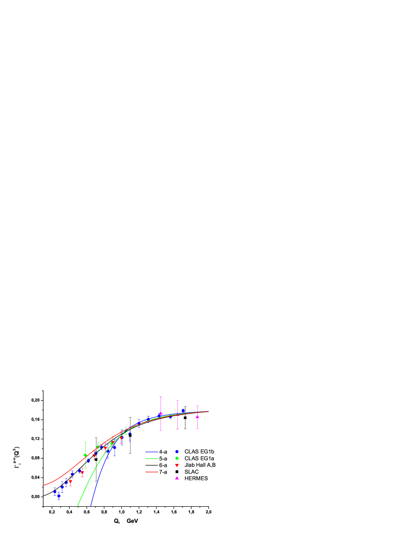
Figure 3: Jlab, SLAC and HERMES experimental data for BSR. The curves represent model predictions obtained for modes with freezing constant $\texttt{N}_{\alpha}=\texttt{4-a}-\texttt{7-a}$ without higher twists (58).

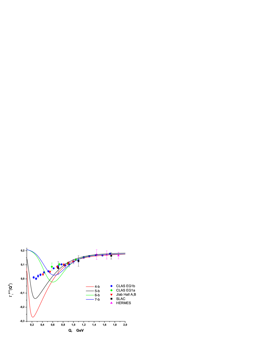
Figure 4: Same as Fig.3, but for constants $\texttt{N}_{\alpha}=\texttt{4-b}-\texttt{7-b}$ with a maximum in the nonperturbative region.

The first conclusion that follows from the calculations is the following: the behavior, in which constants $\alpha\to 0$ when $Q^{2}\to 0$ does not properly describe the experimental data. The highest acceptance probability (minimum $\chi^{2}$) are constants for sets $\texttt{N}_{\alpha}=\texttt{5-{b}}$ and $\texttt{N}_{\alpha}=\texttt{7-{b}}$. Accounting for higher twists does not change this conclusion as well.

As follows from the calculations (see Table 6), models with freezing constant $\texttt{N}_{\alpha}=\nobreak\texttt{6-{a}},\texttt{7-{a}}$ have a minimum of $\chi^{2}$. From Figure 3 one can see that mode $\texttt{N}_{\alpha}=\nobreak\texttt{6-{a}}$ allows us to describe the Bjorken sum rule data.

Let’s briefly consider the contributions of higher-twist to the above conclusions. The results of calculations are given in Table 7 and Figs. 5, 6.

Table 7: Dependence of the $\chi^{2}\left(\texttt{N}_{\alpha}\right)$/D.o.f. on the $3$-parametrers fit results of BSR data with $m_{ht}=0.6\mbox{\leavevmode\nobreak\ GeV}$. The corresponding fit curves are shown in Figs. 5 and 6.

$\texttt{N}_{\alpha}$	$\chi^{2}\left(\texttt{N}_{\alpha}\right)$/D.o.f.	$\texttt{N}_{\alpha}$	$\chi^{2}\left(\texttt{N}_{\alpha}\right)$/D.o.f
4-a	$2.1$	4-b	$1.3$
5-a	$0.7$	5-b	$0.9$
6-a	$0.5$	6-b	$8.4$
7-a	$0.5$	7-b	$5.4$

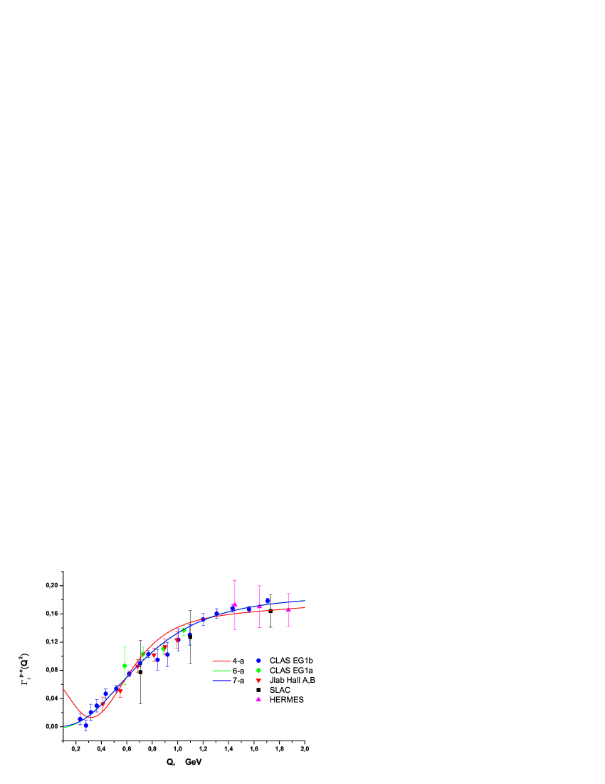
Figure 5: The curves represent model predictions obtained for modes with freezing constant $\texttt{N}_{\alpha}=\texttt{4-a},\texttt{6-a}-\texttt{7-a}$, including higher twists (58) and $m_{ht}=0.6\mbox{\leavevmode\nobreak\ GeV}$

.

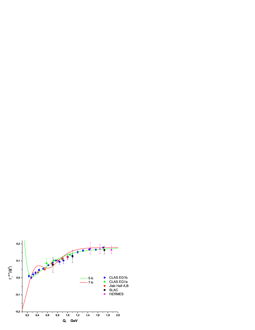
Figure 6: Same as Fig.5, but for constants $\texttt{N}_{\alpha}=\texttt{5-b}$ and $\texttt{N}_{\alpha}=\texttt{7-b}$ with a maximum in the nonperturbative region.

As follows from the calculations, higher twists can improve the agreement between the experimental data and model calculations. However, the smallest $\chi^{2}$ are again constants for $\texttt{N}_{\alpha}=\texttt{6-a}-\texttt{7-a}$.

With the help of (60), (49) and (51) it is easy to estimate the critical value of the strong coupling constant $\alpha_{\mathrm{crit.}}$. If we assume that the value $\Gamma_{1,\mathrm{exp}}^{p-n}(Q^{2})\to 0$ when $Q^{2}\to 0$, and the contribution of higher twists $\Delta_{\mathrm{HT}}^{p-n}\left(Q^{2}=0\right)$ is less than $\sim 0.1$, then, after solving equation

$$C_{NS}\left(Q^{2}=0\right)=0\pm\Delta_{\mathrm{HT}}^{p-n}\left(Q^{2}=0\right)$$ (62)

we find the following numerical estimates

$$\alpha_{\mathrm{crit.}}=0.6861\pm 0.0257\;.$$ (63)

This value is in excellent agreement with constants with $\texttt{N}_{\alpha}=\texttt{6-a}$ and $\texttt{N}_{\alpha}=\texttt{7-a}$ modes.

In this paper, we do not plan to perform detailed calculation of the contributions of higher twists. Note that the fitting procedure shows a strong correlation between the coefficients $\mu_{4},\mu_{6}$ and $\mu_{8}$. Therefore, it is difficultly to reach a clear estimation of the contributions of each of the terms in (58). The solution of this problem is to either reduce the number of parameters to one in $\Delta_{\mathrm{HT}}^{p-n}\left(Q^{2}\right)$ (only $\mu_{4}$) or to search for additional conditions, which limit the values of coefficients $\mu_{4},\mu_{6}$ and $\mu_{8}$.

9 Determination of the “optimal” $\texttt{N}_{\alpha}$ from $\Gamma_{1}^{p,n}$

In this section, we perform a similar procedure for computing estimates of section 8 using the experimental data for the first moment $\Gamma_{1}^{p,n}$.

In order to find the optimal behavior of the simulated mode, we use the combined $\chi^{2}_{\mathrm{com}}\left(\texttt{N}_{\alpha}\right)$:

$$\chi^{2}_{\mathrm{com}}\left(\texttt{N}_{\alpha}\right)=\chi^{2}_{p}\left(\texttt{N}_{\alpha}\right)/D.o.f+\chi^{2}_{n}\left(\texttt{N}_{\alpha}\right)/D.o.f\;,$$ (64)

where

$$\chi^{2}_{p,n}\left(\texttt{N}_{\alpha}\right)=\sum_{i=1}^{k}\frac{\left(\Gamma^{p,n}_{1,\,\mathrm{exp}}(Q^{2}_{i})-\Gamma^{p,n}_{1}(Q^{2}_{i}\right)^{2}}{\left(\delta\Gamma^{p,n}_{1,\,\mathrm{exp}}(Q^{2}_{i})\right)^{2}}\;.$$ (65)

As follows from the calculations (see Figs. 7, 8), to describe the behavior of $\Gamma^{p,n}_{1,\,\mathrm{exp}}(Q^{2})$ one must take into account higher twists, while the contribution $\Delta^{p-n}$ of BSR can be almost neglected (mode $\texttt{N}_{\alpha}=\texttt{6-a}$).

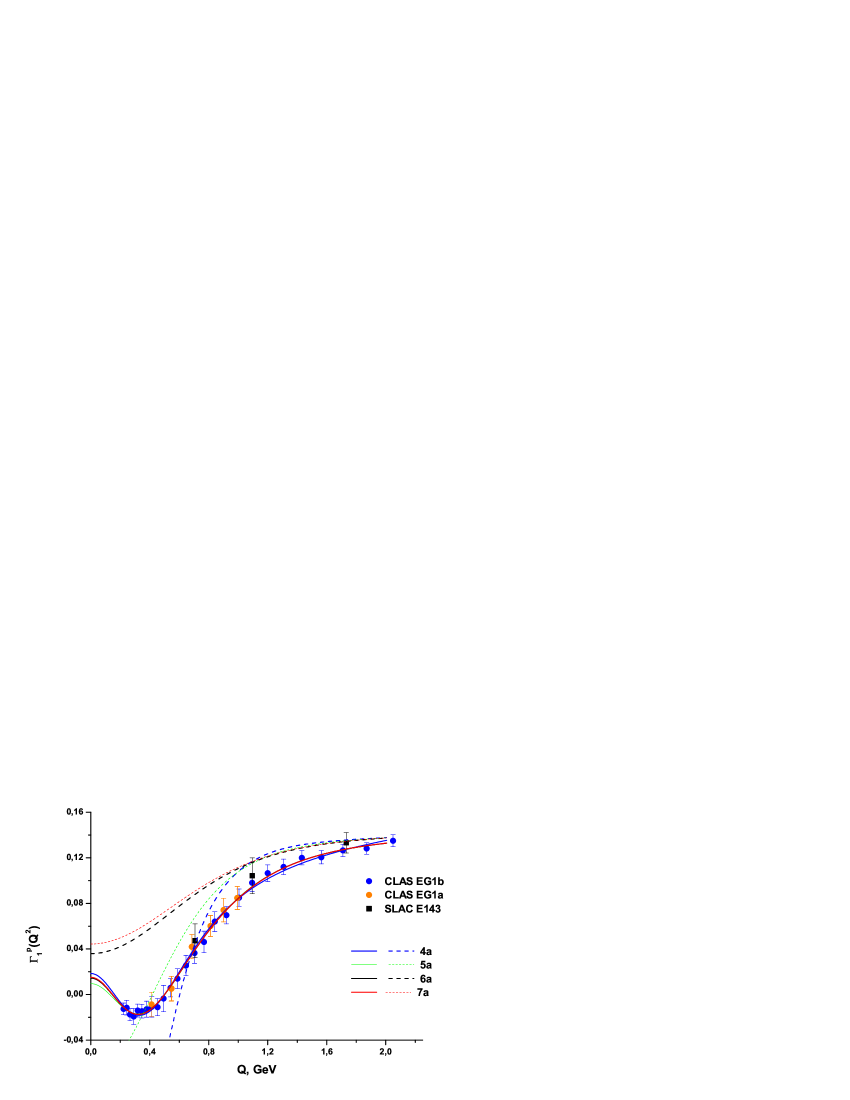
Figure 7: The curves represent model predictions obtained for modes with freezing constant $\texttt{N}_{\alpha}=\texttt{4-a}-\texttt{7-a}$ with (solid lines) and without (dashed lines) higher twists (58) for $m_{ht}=0.6\mbox{\leavevmode\nobreak\ GeV}$.

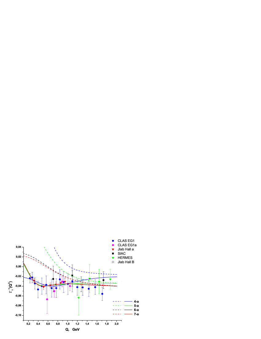
Figure 8: Same as Fig.7, but for $\Gamma_{1}^{n}(Q^{2})$.

The corresponding results for $\chi^{2}_{\mathrm{com}}\left(\texttt{N}_{\alpha}\right)$ with higher twists and without them are listed in Table 8.

Table 8: Dependence of the $\chi^{2}_{com}\left(\texttt{N}_{\alpha}\right)$/D.o.f. on the $4$-parameters fit results of $\Gamma_{1}^{p,n}(Q^{2})$ data with $m_{ht}=0.6\mbox{\leavevmode\nobreak\ GeV}$. The corresponding fit curves are shown in Figs. 7 and 8.

$\texttt{N}_{\alpha}$	$\chi^{2}_{com}\left(\texttt{N}_{\alpha}\right)$/D.o.f.	$\chi^{2}_{com}\left(\texttt{N}_{\alpha}\right)$/D.o.f
	without HT terms	with HT terms
4-a	$482.8$	$0.78$
5-a	$65.1$	$0.43$
6-a	$52.9$	$0.39$
7-a	$63.8$	$0.40$

The parameter $m_{ht}=0.6\mbox{\leavevmode\nobreak\ GeV}$ is chosen so that the result of fitting to the proton $\Gamma_{1}^{p}(Q^{2})$ data for axial charge

$$a_{0}^{inv}=0.325\pm 0.063\;,$$ (66)

is in good agreement with the analysis of COMPASS group [90]

$$a_{0}^{inv}=0.33\pm 0.03(\mbox{stat.})\pm 0.05(\mbox{syst.}).$$

The $Q^{2}$ evolution of the axial singlet charge $a_{0}(Q^{2})$ can now be obtained from Eq.(53) using Eq.(66)

$${a}_{0}(Q^{2}=3\mbox{\leavevmode\nobreak\ GeV}^{2})=0.353\pm 0.069\;,$$

$$a_{0}(Q^{2}=5\mbox{\leavevmode\nobreak\ GeV}^{2})=0.349\pm 0.067\;\;.$$ (67)

Also, the results (67) and experimental values of COMPASS [90]

$${a}_{0}(Q^{2}=3\mbox{\leavevmode\nobreak\ GeV}^{2})=0.35\pm 0.03(\mbox{stat.})\pm 0.05(\mbox{syst.})$$

and HERMES [85] groups

$${a}_{0}(Q^{2}=5\mbox{\leavevmode\nobreak\ GeV}^{2})=0.330\pm\nobreak 0.011(\mathrm{theo.})\pm 0.025(\mathrm{exp.})\pm 0.028(\mathrm{evol.})$$

are consistent with each other.

It is interesting to note that the assumption of conformal invariance [76] improves the agreement between model predictions and experimental data (see Fig. 9). It can serve as an indirect argument for existence of conformal invariant limit of the massless $SU(N_{c})$ gauge model.

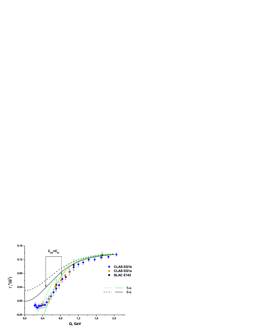
Figure 9: The curves represent the model predictions (without higher twists) $\Gamma_{1}^{p}$ obtained for modes with freezing constant $\texttt{N}_{\alpha}=\texttt{5-a}-\texttt{6-a}$, when $C_{NS}=C_{SI}$ (solid lines) and (dashed lines) when $C_{NS}$, $C_{SI}^{inv}$ are determined by (49), (51) and (50), (52).

10 “Optimal” $\texttt{N}_{\alpha}$ from GLS

The Gross-Llewellyn Smith (GLS) sum rule [91] predicts the integral

$${K}_{GLS}\left(Q^{2}\right)=\frac{1}{2}\int\limits_{0}^{1}F_{3}\left(x,Q^{2}\right)\mathrm{d}x=3\;{C}_{GLS}\left(Q^{2}\right)\;,$$ (68)

where $xF_{3}(x,Q^{2})$ is the nonsinglet structure function measured in $\nu N$-scattering (see [92, 93] and references therein).

The calculation of the $\mathcal{O}\sim\alpha_{s}^{4}$ contribution to $C_{GLS}$ has been published in [94, 40] and the function $C_{GLS}$ can be written in the form

$${C}_{GLS}\left(Q^{2}\right)=C_{NS}\left(Q^{2}\right)+C_{SI}^{GLS}\left(Q^{2}\right)\;,$$ (69)

where the function $C_{NS}\left(Q^{2}\right)$ is determined by Eq.(50) and (52). Singlet contribution is defined by

$$C_{SI}^{GLS}\left(Q^{2}\right)=0.4132\;n_{f}\;a_{s}^{3}(Q^{2})+n_{f}\;(5.802-0.2332\;n_{f})a_{s}^{4}(Q^{2})\;.$$ (70)

Let us compare pQCD results of $K_{GLS}$ with relevant experimental data [93]. We plot the data in Fig. 10 along with model predictions for different variants of $\alpha_{GI}$.

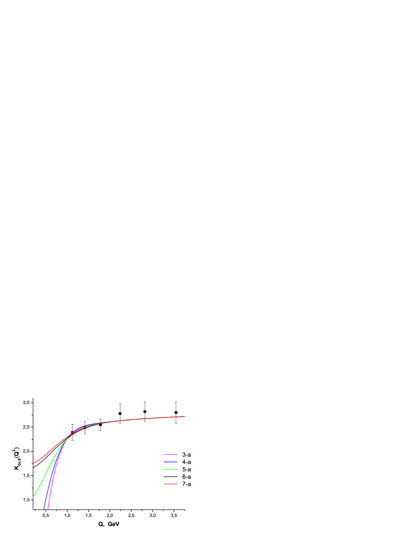
Figure 10: pQCD results of $K_{GLS}$ for different freezing variants of $\alpha_{GI}$.

Within the considerable error bars we see that different versions of $\alpha_{s}$ (21) and experimental data are well compatible with each other in order. To distinguish the behaviour of constants experimental data at lower $Q^{2}<1\mbox{\leavevmode\nobreak\ GeV}$ is needed.

Thus, modern experimental data on the GLS sum rule does not allow to determine the mode of QCD constants behavior.

11 Conclusion

In this paper a method that allows the behavior of the QCD running coupling constant to be assessed in the nonperturbative region is proposed. To study the probable behavior of the QCD constant, 14 regimes were simulated with different $\alpha_{\mathrm{crit.}}=\alpha_{s}\left(0\right)$ and $Q^{2}$ behavior in the nonperturbative region (Tables 1 and 2).

The requirements that underline this method are the matching condition between calculations, which are done within the framework of relativistic quark model (the Poincaré-covariant model) with interquark potential (28), and experimental data on the masses and constants of leptonic decays of pseudoscalar and vector mesons.

Based on the analysis, the compliance with model calculations of the experimental information on the leptonic constants of heavy ($B,D,$ and $D_{s}$) mesons and sum rules of the nucleon can be confirmed. Most appropriate mode is freezing constant with the critical value $\alpha_{\mathrm{crit.}}$ is between $0.65-0.72$ (regimes $\texttt{N}_{\alpha}=\texttt{6-a}$ and $\texttt{N}_{\alpha}=\texttt{7-a}$).

Let us consider what model of freezing strong constant has a similar behavior at small $Q$. These models are:

• MPT coupling constant (9) with $m_{g}=1.0\mbox{\leavevmode\nobreak\ GeV}$, $\alpha_{\mathrm{crit.}}=0.72$ and $\Lambda^{\left(n_{f}=3\right)}=\nobreak 380\mbox{\leavevmode\nobreak\ MeV}$ [10, 12].

• BPT coupling constant (7) with $m_{g}=1.08\mbox{\leavevmode\nobreak\ GeV}$, $\alpha_{\mathrm{crit.}}=0.72$ and $\Lambda^{\left(n_{f}=3\right)}=\nobreak 507\mbox{\leavevmode\nobreak\ MeV}$ [7].

• The nonperturbative effective coupling (13) with $m_{g}=0.34\mbox{\leavevmode\nobreak\ GeV}$, $\alpha_{\mathrm{crit.}}=\nobreak 0.71$ and $\Lambda^{\left(n_{f}=3\right)}=\nobreak 256\mbox{\leavevmode\nobreak\ MeV}$ [4].

• The coupling constant $\alpha_{\rm W}^{(1)}(Q^{2})$ (15) [6] with parameters $c=p=1.71$, $d=0.54$ and $\Lambda^{\left(n_{f}=3\right)}=250\mbox{\leavevmode\nobreak\ MeV}$.

For comparison, the behavior of the effective constants in the nonperturbative region for various approaches and the improved parameterization of mode 6-a are presented in Fig. 11-(b) (right panel). Figure 11-(a) shows model calculations of the Bjorken sum rule without higher twists. As we can see, all these models have is identical behavior in the nonperturbative region, except for the constant (15).

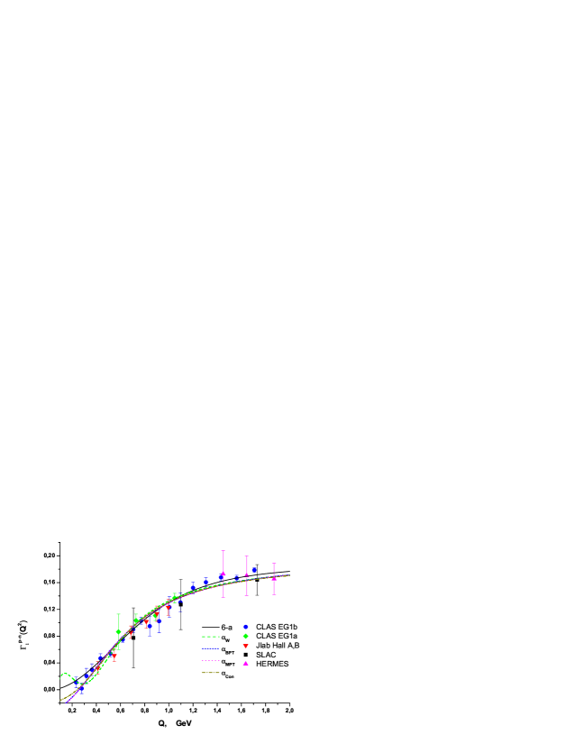
(a) Model predictions of $\Gamma^{p-n}_{1}(Q^{2})$ obtained for modes with freezing constants: $\alpha_{\rm MPT}$ (9), $\alpha_{\rm BPT}$ (7), $\alpha_{\rm Con}$ (13), $\alpha_{\rm Web}$ (15) and mode $\texttt{N}_{\alpha}=\texttt{6-a}$

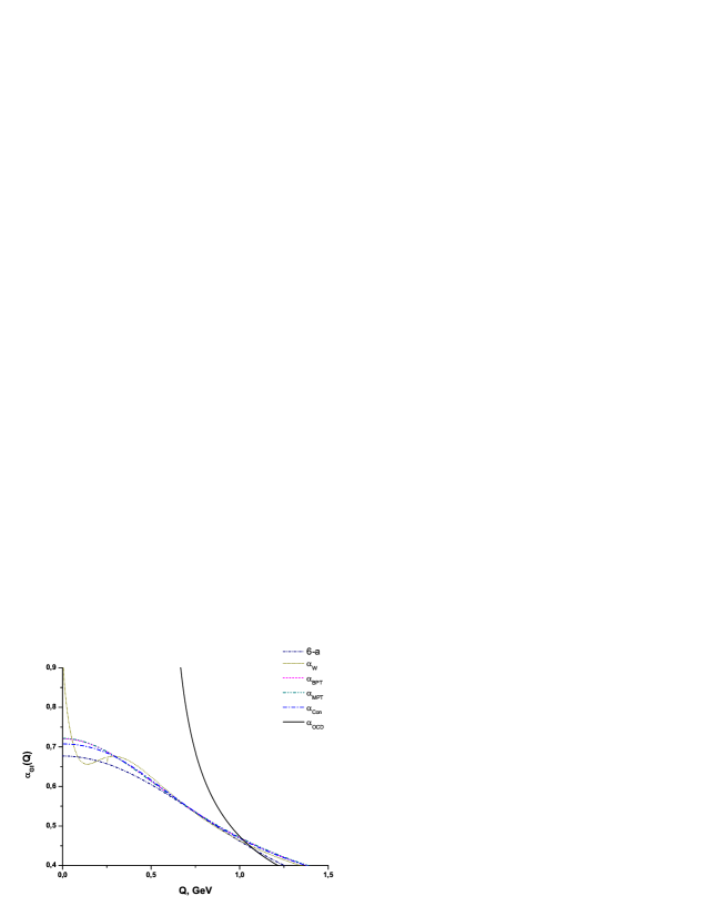
(b) Effective running strong coupling constants: $\alpha_{\rm MPT}$ (9), $\alpha_{\rm BPT}$ (7), $\alpha_{\rm Con}$ (13), $\alpha_{\rm Web}$ (15) and mode $\texttt{N}_{\alpha}=\texttt{6-a}$

Figure 11: Model calculations of the Bjorken sum rule without higher twist and nonperturbative behavior of the various models of effective QCD constants.

I would like to thank O.P. Solovtsova, A.E. Dorokhov, and the attendees of the seminar held at the Laboratory of Theoretical Physics (JINR) for stimulating discussions and advisory comments.

References

- [1] K. Chetyrkin, B. A. Kniehl, and M. Steinhauser, Phys.Rev.Lett. 79, 2184 (1997).
- [2] S. Bethke, Nuclear Physics B Proceedings Supplements 222, 94 (2012).
- [3] J. L. Richardson, Physics Letters 82B, 272 (1979).
- [4] J. M. Cornwall, Phys.Rev. D26, 1453 (1982).
- [5] S. Godfrey and N. Isgur, Phys. Rev. D32, 189 (1985).
- [6] B. R. Webber, JHEP 10, 012 (1998).
- [7] A. M. Badalian and D. S. Kuzmenko, Phys. Rev. D65, 016004 (2002).
- [8] D. V. Shirkov and I. L. Solovtsov, Phys. Rev. Lett. 79, 1209 (1997).
- [9] K. A. Milton, I. L. Solovtsov, and O. P. Solovtsova, Mod. Phys. Lett. A21, 1355 (2006).
- [10] D. Shirkov, Phys.Atom.Nucl. 62, 1928 (1999).
- [11] A. P. Bakulev, S. V. Mikhailov, and N. G. Stefanis, Phys. Rev. D75, 056005 (2007).
- [12] D. V. Shirkov, hep-th/1208.2103 (2012).
- [13] G. Ganbold, Phys. Rev. D 81, 094008 (2010).
- [14] A. Aguilar, D. Binosi, J. Papavassiliou, and J. Rodriguez-Quintero, Phys.Rev. D80, 085018 (2009).
- [15] A. C. Aguilar and J. Papavassiliou, Nucl.Phys.Proc.Suppl. 199, 172 (2010).
- [16] Y. L. Dokshitzer, V. A. Khoze, and S. I. Troian, Phys. Rev. D53, 89 (1996).
- [17] C. S. Fischer, A. Maas, and J. M. Pawlowski, Annals Phys. 324, 2408 (2009).
- [18] V. Bornyakov, E. M. Ilgenfritz, C. Litwinski, V. Mitrjushkin, and M. Muller-Preussker, hep-lat/1302.5943 (2013).
- [19] B. Blossier et al., Phys.Rev. D85, 034503 (2012).
- [20] B. A. Arbuzov, Phys. Lett. B656, 67 (2007).
- [21] B. A. Arbuzov and I. V. Zaitsev, hep-th/1303.0622 (2013).
- [22] A. I. Alekseev and B. A. Arbuzov, Mod. Phys. Lett. A13, 1747 (1998).
- [23] A. I. Alekseev and B. A. Arbuzov, Mod. Phys. Lett. A20, 103 (2005).
- [24] A. V. Nesterenko, Int. J. Mod. Phys. A18, 5475 (2003).
- [25] A. M. Badalian and V. L. Morgunov, Phys. Rev. D60, 116008 (1999).
- [26] M. Peter, Nucl.Phys. B501, 471 (1997).
- [27] Y. S. Kalashnikova, A. V. Nefediev, and Y. A. Simonov, Phys. Rev. D64, 014037 (2001).
- [28] K. A. Milton, I. L. Solovtsov, and O. P. Solovtsova, Phys. Rev. D65, 076009 (2002).
- [29] D. V. Shirkov and I. L. Solovtsov, Theor. Math. Phys. 150, 132 (2007).
- [30] S. Bethke, Eur.Phys.J. C64, 689 (2009).
- [31] S. Bethke, Prog. Part. Nucl. Phys. 58, 351 (2007).
- [32] M. Baldicchi, A. Nesterenko, G. Prosperi, and C. Simolo, Phys.Rev. D77, 034013 (2008).
- [33] M. Baldicchi, A. V. Nesterenko, G. M. Prosperi, D. V. Shirkov, and C. Simolo, Phys. Rev. Lett. 99, 242001 (2007).
- [34] V. Bornyakov, V. Mitrjushkin, and M. Muller-Preussker, Phys.Rev. D81, 054503 (2010).
- [35] P. Boucaud et al., JHEP 04, 006 (2000).
- [36] P. Maris and P. C. Tandy, Phys. Rev. C60, 055214 (1999).
- [37] R. Alkofer, M. Q. Huber, and K. Schwenzer, Eur.Phys.J. C62, 761 (2009).
- [38] D. Binosi and J. Papavassiliou, Phys.Rept. 479, 1 (2009).
- [39] P. Baikov, K. Chetyrkin, and J. Kuhn, Phys.Rev.Lett. 104, 132004 (2010).
- [40] P. Baikov, K. Chetyrkin, J. Kuhn, and J. Rittinger, Phys.Lett. B714, 62 (2012).
- [41] V. V. Andreev, Physics of Particles and Nuclei Letters 8, 347 (2011).
- [42] F. Coester and W. N. Polyzou, Phys. Rev. D26, 1348 (1982).
- [43] B. D. Keister and W. N. Polyzou, Adv. Nucl. Phys. 20, 225 (1991).
- [44] A. Krutov and V. Troitsky, Physics of Particles and Nuclei 40, 136 (2009).
- [45] K. G. Chetyrkin, J. H. Kuhn, and M. Steinhauser, Comput. Phys. Commun. 133, 43 (2000).
- [46] Y. L. Dokshitzer, G. Marchesini, and B. R. Webber, JHEP 07, 012 (1999).
- [47] Y. L. Dokshitzer and B. R. Webber, Phys. Lett. B404, 321 (1997).
- [48] P. A. M. Dirac, Rev. of Modern Phys. 21, 392 (1949).
- [49] V. V. Andreev, Vestsi NAN Belarus, Ser. Fiz. Mat. Nauk , 93 (2000), (in russian.
- [50] A. Krutov, Phys.Atom.Nucl. 60, 1305 (1997).
- [51] W. Jaus, Phys. Rev. D44, 2851 (1991).
- [52] D. Ebert, R. N. Faustov, and V. O. Galkin, Phys. Rev. D62, 034014 (2000).
- [53] E. Balandina, V. Troitsky, A. Krutov, and O. Shro, Phys.Atom.Nucl. 63, 244 (2000).
- [54] J. L. Rosner and S. Stone, hep-ex/0802.1043 (2008).
- [55] J. Beringer and et al., Phys. Rev. D86, 010001 (2012).
- [56] B. Aubert et al., Phys. Rev. D77, 011107 (2008).
- [57] B. Aubert et al., Phys. Rev. D76, 052002 (2007).
- [58] I. Adachi et al., hep-ex/0809.3834 (2008).
- [59] A. J. Schwartz, AIP Conf. Proc. 1182, 299 (2009).
- [60] B. Aubert et al., Phys. Rev. D79, 091101 (2009).
- [61] R. Kowalewski and T. Mannel, (2012), Beringer, J. et al. (Particle Data Group), Phys. Rev. D86, 010001 (2012).
- [62] A. Ali Khan et al., Phys. Lett. B427, 132 (1998).
- [63] A. A. Penin and M. Steinhauser, Phys. Rev. D65, 054006 (2002).
- [64] A. Gray et al., Phys. Rev. Lett. 95, 212001 (2005).
- [65] K. Abe et al., Phys.Rev.Lett. 79, 26 (1997).
- [66] K. Abe et al., Phys.Rev. D58, 112003 (1998).
- [67] M. Amarian et al., Phys.Rev.Lett. 89, 242301 (2002).
- [68] R. Fatemi et al., Phys. Rev. Lett. 91, 222002 (2003).
- [69] A. Deur et al., Phys.Rev.Lett. 93, 212001 (2004).
- [70] K. Dharmawardane et al., Phys.Lett. B641, 11 (2006).
- [71] Y. Prok et al., Phys.Lett. B672, 12 (2009).
- [72] S. Larin, Phys.Lett. B334, 192 (1994).
- [73] A. Kataev, Phys.Rev. D50, 5469 (1994).
- [74] S. Larin, T. van Ritbergen, and J. Vermaseren, Phys.Lett. B404, 153 (1997).
- [75] E. Leader and D. B. Stamenov, Phys.Rev. D67, 037503 (2003).
- [76] A. Kataev, hep-ph/1207.1808 (2012).
- [77] B. Badelek, J. Kwiecinski, and A. Stasto, Z.Phys. 297-306 74, 297 (1997).
- [78] A. V. Kotikov, A. V. Lipatov, and N. P. Zotov, Soviet Journal of Experimental and Theoretical Physics 101, 811 (2005).
- [79] A. Deur, nucl-ex/0508022 (2005).
- [80] R. S. Pasechnik, D. V. Shirkov, O. V. Teryaev, O. P. Solovtsova, and V. L. Khandramai, Phys.Rev. D81, 016010 (2010).
- [81] R. S. Pasechnik, J. Soffer, and O. V. Teryaev, Phys.Rev. D82, 076007 (2010).
- [82] J. Bjorken, Phys.Rev. 148, 1467 (1966).
- [83] J. Bjorken, Phys.Rev. D1, 1376 (1970).
- [84] B. Adeva et al., Phys.Rev. D58, 112002 (1998).
- [85] A. Airapetian et al., Phys.Rev. D75, 012007 (2007).
- [86] A. Airapetian et al., Eur.Phys.J. C26, 527 (2003).
- [87] A. Deur, Chin.Phys. C33, 1261 (2009).
- [88] V. Khandramai, O. Solovtsova, and O. Teryaev, hep-ph/1302.3952 (2013).
- [89] A. V. Kotikov and B. G. Shaikhatdenov, hep-ph/1212.6834 (2013).
- [90] V. Y. Alexakhin et al., Phys.Lett. B647, 8 (2007).
- [91] D. J. Gross and C. H. Llewellyn Smith, Nucl.Phys. B14, 337 (1969).
- [92] I. Hinchliffe and A. Kwiatkowski, Ann.Rev.Nucl.Part.Sci. 46, 609 (1996).
- [93] J. Kim et al., Phys.Rev.Lett. 81, 3595 (1998).
- [94] P. Baikov, K. Chetyrkin, and J. Kuhn, Nucl.Phys.Proc.Suppl. 205-206, 237 (2010).