Statistics of Superior Records

Abstract

We study statistics of records in a sequence of random variables. These identical and independently distributed variables are drawn from the parent distribution $\rho$. The running record equals the maximum of all elements in the sequence up to a given point. We define a superior sequence as one where all running records are above the average record, expected for the parent distribution $\rho$. We find that the fraction of superior sequences $S_{N}$ decays algebraically with sequence length $N$, $S_{N}\sim N^{-\beta}$ in the limit $N\to\infty$. Interestingly, the decay exponent $\beta$ is nontrivial, being the root of an integral equation. For example, when $\rho$ is a uniform distribution with compact support, we find $\beta=0.450265$. In general, the tail of the parent distribution governs the exponent $\beta$. We also consider the dual problem of inferior sequences, where all records are below average, and find that the fraction of inferior sequences $I_{N}$ decays algebraically, albeit with a different decay exponent, $I_{N}\sim N^{-\alpha}$. We use the above statistical measures to analyze earthquake data.

I Introduction

Extreme values are an important feature of data sets, and they are widely used to analyze data in fields ranging from engineering engineer to finance finance1 ; finance2 . For example, the largest and the smallest data points specify the span of the set. Statistical properties of extreme values play a central role in probability theory and in statistical physics wf ; rse ; eig ; book . Studies of extreme value statistics typically focus on average and extremal properties of the distribution of extreme values ft ; eig1 . Yet so far, first passage and persistence properties (see sr ; bms and references therein) have not received significant attention in the context of extreme values.

In this study, we investigate first-passage characteristics of extreme values. Specifically, we compare extreme values with their expected average as a measure of “performance”. We track the record, defined as the largest variable in a sequence of uncorrelated random variables, and ask: what is the probability that all records are “superior”, always outperforming the average. Here, the average refers to the average record that is expected for the particular distribution from which the random variables are drawn. We find that this probability $S_{N}$ decays algebraically with sequence length $N$ (Fig. 1)

$$S_{N}\sim N^{-\beta},$$ (1)

in the large $N$ limit. Interestingly, the decay exponent $\beta$ is nontrivial, being the root of a transcendental equation. When the random variables are drawn from a uniform distribution with compact support in the unit interval, for which the average record equals $N/(N+1)$, we find

$$\beta=0.450265.$$ (2)

In general, the exponent $\beta$ depends on the tail of the probability distribution function from which the random variables are drawn.

Our investigation is motivated by earthquake statistics where extreme values have been recently used to test for correlations among the most powerful earthquake events bp1 ; st ; bdj . We present an empirical analysis of earthquake data that demonstrates how record statistics can be used to analyze the sequence of waiting times between consecutive earthquake events. We also mention that performance statistics have been used to analyze streaks in temperature records ekbhs ; rp ; nmt , and to identify companies that are consistently outperforming the average stock index bp ; lgcmps .

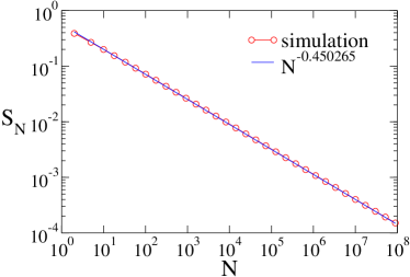
Figure 1: (Color online) The fraction $S_{N}$ of sequences with superior records versus the number of random variables $N$. The random variables are drawn from the uniform distribution (5). The results represent an average over $10^{8}$ independent Monte Carlo realizations.

The rest of this paper is organized as follows. In section II, we analyze statistics of superior records for the basic case of a uniform distribution. We first discuss basic characteristics of records such as the average and the distribution of extreme values, and then derive the exponent (2) using analytic methods. The theoretical description is generalized to arbitrary parent distributions in section III. We discuss in detail the exponential distribution which is later used to analyze earthquake inter-event times and algebraic distributions. The complementary problem of inferior records is discussed in section IV. We use record statistics to analyze earthquake data in section V, and conclude in section VI.

II Uniform Parent Distribution

Consider a set of $N$ independent and identically distributed variables,

$$\{x_{1},x_{2},\ldots,x_{N}\}.$$ (3)

The random variables $x_{i}>0$ are drawn from the probability distribution function $\rho(x)$, and this “parent” distribution is normalized $\int dx\rho(x)=1$. For each sequence of variables, we construct a sequence of running records as follows

$$\{X_{1},X_{2},\ldots,X_{N}\},\qquad X_{n}=\text{max}(x_{1},x_{2},\ldots,x_{n}).$$ (4)

That is, for each $1\leq n\leq N$, the running record $X_{n}$ equals the maximal variable in the sub-sequence $\{x_{1},x_{2},\ldots,x_{n}\}$. Clearly, the sequence of running records is monotonically increasing, $X_{n+1}\geq X_{n}$.

We start by analyzing the simplest possible case of a uniform distribution with compact support in a finite interval. Without loss of generality, we choose the unit interval,

$$\rho(x)=\begin{cases}1&0\leq x\leq 1,\\ 0&x>1.\end{cases}$$ (5)

We define the average running record $A_{N}$ as the expected value of the variable $X_{N}$ over infinitely many realizations, that is, sequences of the type (3) where each variable is drawn from the parent distribution (5). For the uniform distribution, it is easy to see that $A_{1}=1/2$, and similarly, that $A_{2}=2/3$. In general, the average record is

$$A_{N}=\frac{N}{N+1}.$$ (6)

To derive this well-known result, we note that the cumulative probability distribution $R_{N}(x)$ that the running record $X_{N}$ is larger than $x$, is given by

$$R_{N}(x)=1-x^{N}.$$ (7)

Since the probability that one variable is smaller than $x$ equals $x$, then the probability that $N$ variables are smaller than $x$ equals $x^{N}$. This latter probability is complementary to $R_{N}(x)$. The average (6) is obtained from the cumulative distribution (7) by using $A_{N}=-\int_{0}^{1}dx(dR_{N}/dx)\,x$.

In this study, we are primarily interested in the asymptotic behavior when $N\to\infty$. In this limit, $A_{N}\to 1$ and the cumulative distribution $R_{N}(x)$ is appreciable only when $x\to 1$. By rewriting (7) as $R_{N}(x)=1-[1-(1-x)]^{N}$, we see that $R_{N}(x)$ adheres to the scaling form

$$R_{N}(x)\simeq\Psi(s),\quad{\rm with}\quad s=(1-x)\,N.$$ (8)

This form applies when $N\to\infty$ and $1-x\to 0$ such that the product $(1-x)\,N$ is finite, and the scaling function is $\Psi(s)=1-e^{-s}$ ft ; eig1 .

We term a record sequence $(X_{1},X_{2},\ldots,X_{N})$ superior when all records are above average, that is,

$$X_{n}>A_{n}\quad\text{for all}\quad n=1,2,\ldots,N.$$ (9)

For example, for the uniform distribution, a record sequence is superior if all of the following $N$ conditions are met: $x_{1}>1/2$, ${\rm max}(x_{1},x_{2})>2/3$, $\ldots$, ${\rm max}(x_{1},x_{2},\ldots,x_{N})>N/(N+1)$. We are interested in the probability $S_{N}$ that a record sequence of length $N$ is superior. This quantity is reminiscent of a survival probability sr since we require that a certain threshold, defined by the average, is never crossed.

To find $S_{N}$, we have to incorporate the value of the record into our theoretical description. We define $F_{N}(x)$ as the fraction of record sequences of length $N$ that are: (i) superior, that is, $X_{n}>A_{n}$ for all $n\leq N$ and (ii) have extreme value larger than $x$, namely, $X_{N}>x$. The cumulative distribution $F_{N}(x)$ is applicable when $x>A_{N}$, and moreover $F_{N}(\tfrac{N}{N+1})=S_{N}$ and $F_{N}(1)=0$.

The cumulative distribution obeys the recursion

$$F_{N+1}(x)=x\,F_{N}(x)+(1-x)\,S_{N}$$ (10)

for all $x>A_{N+1}$. This recursion equation reflects that there are two possibilities: The $(N+1)$st element in the sequence may set a new record, or alternatively, the old record may hold. The second term corresponds to the former scenario, and the first term to the latter. Of course, for the uniform distribution, the probability that the record holds is equal to the value of the record.

Since the first variable necessarily sets a record, $X_{1}=x_{1}$, we have $F_{1}(x)=1-x$. Using the recursion relation (10) we obtain

$$F_{1}(x) = 1-x$$

$$F_{2}(x) = \frac{1}{2}\left(1+x-2x^{2}\right),$$

$$F_{3}(x) = \frac{1}{18}\left(7+2x+9x^{2}-18x^{3}\right),$$

$$F_{4}(x) = \frac{1}{576}\left(191+33x+64x^{2}+288x^{3}-576x^{4}\right).$$

In general, the distribution $F_{N}(x)$ is a polynomial of degree $N$. Using $S_{N}=F_{N}(\tfrac{N}{N+1})$ we obtain the probabilities

$$S_{1}=\frac{1}{2},\quad S_{2}=\frac{7}{18},\quad S_{3}=\frac{191}{576},\quad S_{4}=\frac{35393}{120000}.$$

The scaling behavior (8) suggests that the polynomials $F_{N}(x)$ approach a universal function of the scaling variable $s=N(1-x)$ when $N\to\infty$. As shown in figure 2, the first four polynomials support this assertion. We thus seek a scaling solution in the form

$$F_{N}(x)\simeq S_{N}\Phi(s),\quad s=(1-x)N.$$ (11)

By definition, $F_{N}(\tfrac{N}{N+1})=S_{N}$, and hence, $\Phi(1)=1$. The cumulative distribution vanishes when $x\to 1$, and hence $\Phi(0)=0$. The variable $s$ has the range $0\leq s\leq 1$ with the upper bound corresponding to near-average records and the lower bound, to extremely large records.

To determine the scaling function $\Phi(s)$, we treat $N$ as a continuous variable, and convert the difference equation (10) into an evolution equation. The cumulative distribution obeys the difference equation $F_{N+1}-F_{N}=(1-x)(S_{N}-F_{N})$, where $F_{N}\equiv F_{N}(x)$ and hence, when $N$ is large, can be replaced by the partial differential equation

$$\frac{\partial F_{N}}{\partial N}=(1-x)\,(S_{N}-F_{N}).$$ (12)

Essentially, this is as an evolution equation with the sequence length $N$ playing the role of time.

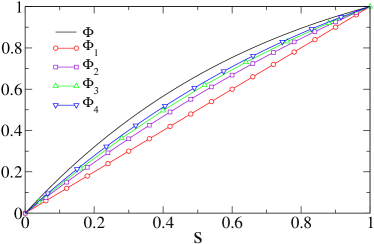
Figure 2: (Color online) The scaling behavior (11). Shown are the normalized polynomials $\Phi_{N}=F_{N}/S_{N}$ versus the variable $s$ for $N\leq 4$. Also shown for reference is the scaling function (14).

By substituting the scaling form (11) into the evolution equation (12) and by using the algebraic decay (1), we find that the scaling function $\Phi(s)$ obeys the differential equation

$$\Phi^{\prime}(s)+(1-\beta\,s^{-1})\Phi(s)=1.$$ (13)

We integrate this equation by multiplying both sides by the integrating factor $s^{-\beta}e^{s}$. Given the boundary condition $\Phi(0)=0$, we obtain $\Phi(s)=s^{\beta}e^{-s}\int_{0}^{s}du\,u^{-\beta}e^{u}$, and this expression can be further simplified to

$$\Phi(s)=s\,\int_{0}^{1}dz\,z^{-\beta}e^{s(z-1)}.$$ (14)

By invoking the boundary condition $\Phi(1)=1$, we find the exponent $\beta$ as the root of the transcendental equation

$$\int_{0}^{1}dz\,z^{-\beta}e^{(z-1)}=1.$$ (15)

This equation gives the exponent $\beta$ quoted in (2). The expressions (15) and (14) give the asymptotic fraction of superior sequences and the extreme value distribution for such sequences.

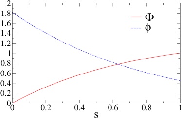
Figure 3: (Color online) The scaling functions $\Phi(s)$ and $\phi(s)=\Phi^{\prime}(s)$ versus the scaling variable $s$ for $\alpha=1$

The scaling function $\Phi(s)$ that underlies the cumulative distribution of extreme values is shown in figure 3. Also shown is the derivative $\phi(s)=\Phi^{\prime}(s)$ that characterizes the distribution $f_{N}=-dF_{N}/dx$. Equation (11) implies the scaling behavior

$$f_{N}(x)\simeq N\,S_{N}\,\phi(s)$$ (16)

with $s=(1-x)N$. From (13), we obtain $\phi(0)=1/(1-\beta)$ and $\phi(1)=\beta$. The distribution $\phi(s)$ decreases monotonically with $s$. One also finds that the average record for a superior sequence, $\langle x\rangle=\int_{0}^{1}dxf_{N}(x)\,x$, behaves as

$$1-\langle x\rangle\simeq a\,N^{-1},\qquad a=1-\int_{0}^{1}ds\,\Phi(s).$$ (17)

Since the scaled distribution function $\phi(s)$ is monotonically decreasing (see Fig. 3) we expect $a<1/2$, and indeed $a=0.388476$. Consequently, the average record is closer to unity than it is to the average ($1-A_{N}\simeq N^{-1}$).

III General Parent Distributions

Generalization of the above results to arbitrary distribution $\rho(x)$ is straightforward. Let us consider the general case when the random variables $0<x_{i}<\infty$ are drawn from the distribution $\rho(x)$, with the normalization $\int_{0}^{\infty}dx\rho(x)=1$. The cumulative distribution

$$R(x)=\int_{x}^{\infty}dy\rho(y)$$ (18)

gives the probability of drawing a value larger than $x$, with $R(0)=1$ and $R(\infty)=0$.

The probability $R_{N}(x)$ that the record is larger than $x$ follows immediately from the cumulative distribution,

$$R_{N}(x)=1-\left[1-R(x)\right]^{N}.$$ (19)

Indeed, the complementary probability that all variables are smaller than $x$, and hence the record is smaller than $x$, is $[1-R(x)]^{N}$ since the random variables are independent. In the limit $N\to\infty$, the quantity (19) adheres to the scaling form

$$R_{N}(x)\simeq\Psi(s),\quad{\rm with}\quad s=N\,R(x).$$ (20)

This form applies when $N\to\infty$ and $R\to 0$ with the product $R\,N$ finite. Importantly, the scaling function is the same, $\Psi(s)=1-e^{-s}$, for all parent distributions ft ; eig1 .

The average record is given by $A_{N}=-\int_{0}^{\infty}dx\,x\,\frac{dR_{N}}{dx}$. Inserting (19) into this integral yields the average in terms of the cumulative distribution,

$$A_{N}=N\int_{0}^{1}dR\,(1-R)^{N-1}x,$$ (21)

where $x=x(R)$ is implicitly given by Eq. (18).

We again characterize superior sequences using the cumulative distribution $F_{N}(x)$ which obeys the recursion

$$F_{N+1}(x)=\left[1-R(x)\right]\,F_{N}(x)+R(x)\,S_{N}$$ (22)

for all $x>A_{N+1}$. This equation is obtained from (10) by replacing $1-x$ with the general form $R(x)$. Starting with $F_{1}=1-R$, we find that $F_{N}$ is a polynomial of degree $N$ in the quantity $R\equiv R(x)$. For example, $F_{2}=R(1+R_{1}-R)$ with the shorthand notation

$$R_{N}\equiv R(A_{N}).$$ (23)

Further, the evolution equation (12) is now

$$\frac{\partial F_{N}}{\partial N}=R\,(S_{N}-F_{N}).$$ (24)

Therefore, we seek the scaling solution

$$F_{N}(x)\simeq S_{N}\Phi(s),\quad{\rm with}\quad s=N\,R(x).$$ (25)

By definition, $F_{N}(A_{N})=S_{N}$, and hence, $\Phi(\alpha)=1$ where

$$\alpha=\lim_{N\to\infty}N\,R_{N},$$ (26)

with $R_{N}$ given in (23). Remarkably, all details of the parent distribution enter through the parameter $\alpha$ which dictates the boundary condition, $\Phi(\alpha)=1$. The second boundary condition remains $\Phi(0)=0$. Since $R\to 0$ when $N\to\infty$, equation (26) shows that the tail of the probability distribution function $\rho(x)$ determines the parameter $\alpha$. Indeed, the term $(1-R)^{N-1}$ in (21) effectively involves only the tail of $R(x)$ when $N\to\infty$.

By substituting the scaling form (25) into the evolution equation (24) and by using the algebraic decay (1), we find that the scaling function $\Phi(s)$ obeys the differential equation (13). The solution is given by (14) and the boundary condition $\Phi(\alpha)=1$ yields the exponent $\beta$ as root of the transcendental equation

$$\alpha\int_{0}^{1}dz\,z^{-\beta}e^{\alpha(z-1)}=1.$$ (27)

This equation specifies the exponent $\beta$ and hence, the scaling function $\Phi(s)$ given in (14).

For arbitrary $\rho(x)$, the expressions (27) and (14) give the asymptotic fraction of superior sequences and the extreme-value distribution for such sequences. These equations require as input the parameter $\alpha$ defined in (26) which in turn, requires the average $A_{N}$ given in (21). We now apply the general theory above to: (i) exponential distributions, both simple and generalized, and (ii) algebraic distributions, both compact and noncompact.

First, we consider the exponential distribution which characterizes the waiting times in a Poisson process where events are uncorrelated and occur at a constant rate in time ngv

$$\rho(x)=e^{-x}.$$ (28)

This distribution is relevant for the empirical analysis presented in section IV. In this special case, the probability distribution and the cumulative distribution are identical, $R(x)=\rho(x)$. According to Eq. (21), the average $A_{N}=-N\int_{0}^{1}dR\,(1-R)^{N-1}\ln R$ is equals to the harmonic number

$$A_{N}=1+\frac{1}{2}+\frac{1}{3}+\cdots+\frac{1}{N}.$$ (29)

From the cumulative distribution $R(x)=\exp(-x)$ we simply have $R_{N}=\exp(-A_{N})$. Using the asymptotic behavior $A_{N}\simeq\ln N+\gamma$, where $\gamma=0.577215$ is the Euler constant Knuth , we obtain

$$\alpha=e^{-\gamma}.$$ (30)

Plugging the corresponding numerical value $\alpha=0.561459$ into the integral equation (15) gives

$$\beta=0.621127.$$ (31)

The behavior found for the exponential distribution extends to all distribution with the generalized exponential tail

$$R(x)\simeq C\exp(-x^{c})$$ (32)

with $C>0$ and $c>0$ when $x\to\infty$. As discussed above, the parameter $\alpha$ requires as input only the tail of the distribution $R(x)$. By substituting (32) into the general formula (21) and writing $R=r/N$ we have,

$$A_{N}=N\int_{0}^{N}dr\left(1-\frac{r}{N}\right)^{N-1}\left[\ln(NC/r)\right]^{1/c}.$$

The leading asymptotic behavior of this integral can be evaluated using the integral $\int_{0}^{\infty}dr\,e^{-r}\ln r=-\gamma$ as follows,

$$A_{N} \simeq \int_{0}^{\infty}dr\,e^{-r}\left[\ln(NC/r)\right]^{1/c}$$

$$\simeq \int_{0}^{\infty}dr\,e^{-r}\left[\ln(NC)\right]^{1/c}\left(1-\frac{\ln r}{\ln(NC)}\right)^{1/c}$$

$$\simeq \left[\ln(NC)\right]^{1/c}\left(1+\frac{\gamma}{c}\frac{\ln r}{\ln(NC)}\right).$$

Hence, we observe the generic result $(A_{N})^{c}\simeq\ln(NC)+\gamma$. By specializing the general expression (26) to the distribution (32), we obtain

$$\alpha=\lim_{N\to\infty}NC\,\exp\left[-(A_{N})^{c}\right]=e^{-\gamma}.$$ (33)

Hence, the exponent $\alpha$ given in (26) holds for all values of $c$, and hence, for all generalized exponential distributions.

Next, we consider algebraic distribution functions. We first consider distributions with compact support in a finite interval, taken as the unit interval $[0:1]$ without loss of generality. The behavior near the maximum plays a crucial role, and we consider a class of distributions that exhibit the algebraic behavior,

$$R(x)\simeq B(1-x)^{\mu},$$ (34)

with $\mu>0$ in the limit $x\to 1$. The restriction on $\mu$ ensures that the distribution $\rho=-dR/dx$ is integrable. The case $\mu=1$ corresponds to the uniform distribution studied above. Using the general formula (21), we obtain the large-$N$ asymptotic behavior of the average

$$1-A_{N}\simeq\Gamma\big{(}1+\tfrac{1}{\mu}\big{)}\,(BN)^{-\frac{1}{\mu}}$$ (35)

The exponent $\alpha$ can be obtained using equations (23), (26), and (35),

$$\alpha=\left[\Gamma\big{(}1+\tfrac{1}{\mu}\big{)}\right]^{\mu}.$$ (36)

By substituting $\alpha$ into the integral equation (15), we obtain the exponent $\beta$. As shown in figure 4, the exponent $\beta$ varies continuously with $\mu$ bkr ; kj . The exponent $\mu$ parametrizes the shape of the distribution near the maximum. As suggested by equation (26), the tail of the distribution $\rho(x)$ governs the exponent $\beta$.

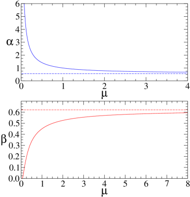
Figure 4: (Color online) The exponents $\alpha$ (top figure) and $\beta$ (bottom figure) versus the parameter $\mu$. The dashed lines indicate the lower bound $\alpha_{\rm min}=0.561459$ and upper bound $\beta_{\rm max}=0.621127$, respectively.

Using the asymptotic behavior $\Gamma(1+\epsilon)\simeq 1-\gamma\epsilon$ for $\epsilon\to 0$ with $\gamma$ the Euler constant, we obtain

$$\alpha=\left[\Gamma\big{(}1+\tfrac{1}{\mu}\big{)}\right]^{\mu}\to\left[1-\tfrac{\gamma}{\mu}\right]^{\mu}\to e^{-\gamma}$$

when $\mu\to\infty$. Hence, the behavior in the limit $\mu\to\infty$ coincides with that of the generalized exponential distribution (32). Figure 4 shows that the parameter $\alpha$ decreases monotonically with $\mu$ while the exponent $\beta$ increases monotonically with $\mu$. Hence, the value (30) is a lower bound, $\alpha_{\rm min}\leq\alpha<\infty$, while that quoted in (31) is an upper bound, $0<\beta\leq\beta_{\rm max}$.

Finally, the parameter (36) extends to non-compact distributions with algebraic tails, $R(x)\simeq b\,x^{\mu}$ when $x\to\infty$. The condition $\mu<-1$ guarantees that the average is finite. In this case, we have $A_{N}\simeq(bN/\alpha)^{-1/\mu}$ with the $\alpha$ given in (36). Therefore, the exponent $\beta$ shown in figure 4 holds for non-compact distribution with power-law tails.

IV Inferior Records

We briefly discuss the dual probability $I_{N}$ that all records are inferior, that is, they are below average: $X_{n}<A_{n}$ for all $n\leq N$. For example, for the uniform distribution (5) we require that $N$ conditions are met: $X_{1}<1/2$, $X_{2}<2/3$, $\ldots$, $X_{N}<N/(N+1)$. For the uniform distribution (5), the probability $I_{N}$ has an especially simple form. First, we note that $I_{1}=1/2$. The probability that $x_{1}<1/2$ and ${\rm max}(x_{1},x_{2})<2/3$ is simply $I_{2}=(1/2)\times(2/3)=1/3$. In general, we have

$$I_{N}=\frac{1}{2}\times\frac{2}{3}\cdots\times\frac{N}{N+1}=\frac{1}{N+1}.$$ (37)

Asymptotically, the quantity $I_{N}$ is inversely proportional to sequence length, $I_{N}\sim N^{-1}$.

In general the probability $I_{N}$ obeys the recursion

$$I_{N+1}=I_{N}(1-R_{N+1}),$$ (38)

with $I_{1}=1-R_{1}$. The factor $1-R_{N+1}$ guarantees that the record $X_{N+1}$ is inferior, regardless of the history of the sequence. In contrast with the recursion (10), the probability $I_{N}$ obeys a closed equation. The solution is the product

$$I_{N}=(1-R_{1})\,(1-R_{2})\,\cdots\,(1-R_{N}).$$ (39)

This general expression generalizes (37).

To obtain the asymptotic behavior for an arbitrary distribution, we convert the difference equation (38) into the differential equation $dI/dN=-\alpha\,I/N$. The probability $I$ decays algebraically,

$$I\sim N^{-\alpha},$$ (40)

with the exponent $\alpha$ given by (26). Indeed, for the uniform distribution, we recover $\alpha=1$. Once again, the tail of the distribution $\rho(x)$ controls the exponent $\alpha$ (see also figure 4). Hence, the probabilities $S_{N}$ and $I_{N}$ that measure the fraction of superior and inferior sequences decay algebraically, each with a different exponent. The decay exponents are generally nontrivial.

V Records in Earthquake Data

In this section, we analyze earthquake data using the record statistics discussed above. The surge in the number of powerful earthquakes over the past decade rak raises the question whether powerful earthquakes are correlated in time along with the possibility that one large earthquake may trigger another large earthquake at a global distance bp . Temporal correlations necessarily imply that earthquake events do not occur randomly in time gk . Using a variety of statistical tests, the sequence of most powerful events was compared with a Poisson process where events occur randomly and at a constant rate. The results largely reaffirm that the earthquake record is consistent with a Poisson process am ; st ; dbgj ; bdj .

These statistical tests typically use the inter-event time, defined as the time between two successive events am ; st ; bdj . For a Poisson process, the distribution of inter-event times is exponential as in (28), where the normalization $\langle x\rangle=1$ is conveniently used. Recent studies show that the empirical distribution $\rho(x)$ is close to an exponential am ; bdj . Moreover, statistical properties of the maximal inter-event time are consistent with Poisson statistics st ; bdj .

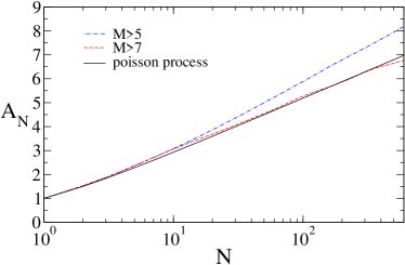
Figure 5: (Color online) The average record versus sequence length. Shown are empirical results for the earthquakes with magnitude $M>7$ and for earthquakes with magnitude $M>5$. Also shown for a reference is the harmonic number (29) that corresponds to Poisson process.

Previous studies utilized a single record, the maximal inter-event time. Here, we utilize the entire sequence of records $\{X_{1},X_{2},\ldots,X_{N}\}$ defined in equation (4) which is produced from the sequence of inter-event times $\{x_{1},x_{2},\ldots,x_{N}\}$ where $x_{i}$ is the time between the $i$th and the $i+1$th earthquake events. In particular, we measure the average record $A_{N}$ as a function of the number of consecutive earthquake events $N$.

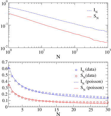
Figure 6: (Color online) The probabilities $S_{N}$ and $I_{N}$ for the earthquake sequence with $M>7$ (bottom figure) and $M>5$ (top figure). The empirical results for $M>7$ are compared with the theoretical predictions (10) and (39) with $R_{N}=\exp(-A_{N})$ with $A_{N}$ given in (29).

We considered two separate datasets data . A global record of $1770$ earthquakes with magnitude $M>7$ during the years $1900-2012$ and a global record of $37,190$ events with magnitude $M>5$ during the years $1984-2012$. According to the Gutenberg-Richter law, the rate of events decreases exponentially with magnitude, defined as the logarithm of the energy released in the earthquake gr . On average, roughly 16 magnitude $M>7$ events occur each year, while there are about $1300$ magnitude $M>5$ events annually. The first sequence of most powerful events with $M>7$ includes few aftershocks and is expected to be Poissonian. The second sequence with $M>5$ includes many aftershocks, which are certainly correlated events, and is expected to be non Poissonian sus . As shown in figure 5, the average record closely tracks the harmonic number when $M>7$, but there is a clear departure from Poisson statistics for the less powerful events ($M<5$). We note the utility of the average record as the quantity $A_{N}$ can be analyzed over a range that is comparable with the total number of events.

Next, we measured the probabilities $S_{N}$ and $I_{N}$ that a sequence of $N$ records is superior or inferior. To obtain these probabilities, we simply used the averages shown in figure 6. For powerful events ($M>7)$ where the number of events is relatively small, these quantities can be measured only over a small range, but nevertheless, the results are consistent with the behavior expected for a random sequence of events. For $M>5$, the number of events is much larger and we can confirm that the probabilities $S_{N}$ and $I_{N}$ decay algebraically with the exponents $\alpha=0.38\pm 0.05$ and $\beta=0.46\pm 0.05$ (figure 6). These values are somewhat smaller than the extremal values $\alpha_{\rm min}$ and $\beta_{\rm max}$ that correspond to sharper-than-algebraic tails.

VI Conclusions

In summary, we studied statistics of superior records in a sequence of uncorrelated random variables. In our definition, a sequence of records is superior if all records are above average. We presented a general theoretical framework that applies for arbitrary probability distribution functions, and used scaling methods to analyze the asymptotic behavior of large sequences. We obtained analytically the distribution of records and the fraction of superior sequences. The latter quantity decays algebraically with sequence length. Interestingly, the decay exponent is nontrivial, and it is controlled by the tail of the probability distribution function from which the random variables are drawn.

We demonstrated that there are two separate exponents that characterize inferior and superior sequences. The first exponent simply measures the weight of the probability distribution beyond the average record, while the second exponent is derived through an integral equation from the first exponent. In general, both of these exponents are irrational. The tail of the parent distribution function dictates the exponents: for algebraic distributions, the exponents continuously vary with the decay coefficient governing the tail of the parent distribution, while parent distributions with sharper-than-algebraic tails all have the same exponents.

Our results show that first-passage properties of records are quite rich. Our study compares the actual record with the average expected for a given distribution as a probe of performance. Yet, performance is only one in a larger family of characteristics involving the entire history of the sequence. Our results suggest that there are additional “persistence”-like exponents dhp ; msbc for record sequences. Finally, it will be interesting to investigate superior records in sequences of correlated random variables, e.g. when the sequence $x_{n}$ represents a random walk wms ; wbk .

We also demonstrated that record and performance statistics are useful for analyzing empirical data. For instance, the average record is a transparent statistical test for whether a sequence of events is random in time. The probability that a sequence of records is superior or inferior can be measured as well. However, since these survival probabilities decay algebraically, very large datasets are required. Nevertheless, the earthquake data demonstrates that these are sensible quantities for analyzing datasets.

- (1) E. Castillo, Extreme Value Theory in Engineering (Academic Press, New York, 1988).
- (2) P. Embrechts, G. Klüppelberg and T. Mikosch, Modelling extremal events for insurance and finance (Spring-Verlag, Berlin, 1997).
- (3) S. Y. Novak, Extreme value methods with applications to finance (Chapman & Hall/CRC Press, London, 2011).
- (4) W. Feller, An Introduction to Probability Theory and Its Applications (Wiley, New York, 1968).
- (5) R. S. Ellis, Entropy, Large Deviations, and Statistical Mechanics (Springer, Berlin 2005).
- (6) E. I. Gumbel, Statistics of Extremes (Dover, New York 2004).
- (7) P. L. Krapivsky, S. Redner and E. Ben-Naim, A Kinetic View of Statistical Physics (Cambridge University Press, Cambridge, UK, 2010).
- (8) R. A. Fisher and L. H. C.Tippett, Proc. Cambridge Phil. Soc. 24, 180 (1928).
- (9) E. I. Gumbel, Ann. Inst. Henri Poincaré 5, 115 (1935).
- (10) S. Redner, A Guide to First-Passage Processes (Cambridge University Press, New York, 2001).
- (11) A. J. Bray, S. N. Majumdar, and G. Schehr, Persistence and First-Passage Properties in Non-equilibrium Systems, arXiv:1304.1195.
- (12) C. G. Bufe and D. M. Perkins Seismol. Res. Lett. 82, 455 (2011).
- (13) P. M. Shearer and P. B. Stark, Proc. Nat. Acad. Sci. 109, 717 (2012).
- (14) E. Ben-Naim, E. G. Daub, and P. A. Johnson, Geophys. Res. Lett. 40, L50605 (2013).
- (15) J. F. Eichner, E. Koscielny-Bunde, A. Bunde, S. Havlin, H. J. Schellnhuber, Phys. Rev. E 68, 046133 (2003).
- (16) S. Redner and M. R. Petersen, Phys. Rev. E 74, 061114 (2006).
- (17) W. I. Newman, B. D. Malamud, and D. L. Turcotte, Phys. Rev. E 82, 066111 (2010).
- (18) J.-P. Bouchaud and M. Potters, Theory of Financial Risk and Derivative Pricing (Cambridge University Press, Cambridge 2003).
- (19) Y. H. Liu, P. Gopikrishnan, P. Cizeau, M. Meyer, C. K. Peng, and H. E. Stanley, Phys. Rev. E 60, 1390 (1999).
- (20) N. G. van Kampen, Stochastic Processes in Physics and Chemistry (North-Holland, Amsterdam, 2001).
- (21) R. L. Graham, D. E. Knuth, and O. Patashnik, Concrete Mathematics : A Foundation for Computer Science (Reading, Mass.: Addison-Wesley, 1989).
- (22) E. Ben-Naim, P. L. Krapivsky, and S. Redner, Phys. Rev. E 50, 822 (1994).
- (23) J. Krug and K. Jain, Physica A 358, 1 (2005).
- (24) R. A. Kerr, Science 332, 411 (2011).
- (25) J. Gardner and L. Knopoff, Bull. Seismol. Soc. Am. 64, 1363 (2011).
- (26) A. J. Michael, Geophys. Res. Lett. 38, L21301 (2012).
- (27) E. G. Daub, E. Ben-Naim, R. A. Guyer, and P. A. Johnson, Geophys. Res. Lett. 39, L06308 (2012).
- (28) The earthquake catalog are available from: http://earthquake.usgs.gov/earthquakes/pager/ and http://earthquake.usgs.gov/monitoring/anss/.
- (29) B. Gutenberg and C. F. Richter, Seismicity of the Earth and Associated Phenomena (Princeton University Press, Princeton, 1954)
- (30) D. Sornette, S. Utkin, and A. Saichev, Phys. Rev. E 77, 066109 (2008).
- (31) B. Derrida, V. Hakim, and V. Pasquier, Phys. Rev. Lett. 75, 751 (1995).
- (32) S. N. Majumdar, C. Sire, A. J. Bray, and S. J. Cornell, Phys. Rev. Lett. 77, 2867 (1996); B. Derrida, V. Hakim, and R. Zeitak, Phys. Rev. Lett. 77, 2871 (1996).
- (33) G. Wergen, S. N. Majumdar, and G. Schehr, Phys. Rev. E 86, 011119 (2012); G. Schehr and S. N. Majumdar, arXiv:1305.0639.
- (34) G. Wergen, M. Bogner, and J. Krug, Phys. Rev. E 83, 051109 (2011).