Luminosities of Carbon-rich Asymptotic Giant Branch stars in the Milky Way

Abstract

Context. Stars evolving along the Asymptotic Giant Branch can become Carbon-rich in the final part of their evolution. They replenish the inter-stellar medium with nuclear processed material via strong radiative stellar winds. The determination of the luminosity function of these stars, even if far from being conclusive, is extremely important to test the reliability of theoretical models. In particular, strong constraints on the mixing treatment and the mass-loss rate can be derived.

Aims. We present an updated Luminosity Function of Galactic Carbon Stars obtained from a re-analysis of available data already published in previous papers.

Methods. Starting from available near- and mid-infrared photometric data, we re-determine the selection criteria. Moreover, we take advantage from updated distance estimates and Period-Luminosity relations and we adopt a new formulation for the computation of Bolometric Corrections. This leads us to collect an improved sample of carbon-rich sources from which we construct an updated Luminosity Function.

Results. The Luminosity Function of Galactic Carbon Stars peaks at magnitudes around $-$4.9, confirming the results obtained in a previous work. Nevertheless, the Luminosity Function presents two symmetrical tails instead of the larger high luminosity tail characterizing the former Luminosity Function.

Conclusions. The derived Luminosity Function of Galactic Carbon Stars matches the indications coming from recent theoretical evolutionary Asymptotic Giant Branch models, thus confirming the validity of the choices of mixing treatment and mass-loss history. Moreover, we compare our new Luminosity Function with its counterpart in the Large Magellanic Cloud finding that the two distributions are very similar for dust-enshrouded sources, as expected from stellar evolutionary models. Finally, we derive a new fitting formula aimed to better determine Bolometric Corrections for C-stars.

1 Introduction

After the exhaustion of their central helium, stars with initial masses between 0.8 and 8 M_⊙ evolve through the Asymptotic Giant Branch phase (hereafter AGB). These stars efficiently pollute the Inter-Stellar Medium (hereafter ISM) by ejecting their cool and expanded envelopes via strong stellar winds powered by radial pulsations and radiation pressure on dust grains. Moreover, being extremely luminous objects, they provide the dominant contribution to the integrated light of aged stellar populations. A detailed modeling of their theoretical evolution and an extensive study of their observational properties is therefore mandatory.

During the AGB phase, nuclear processed material from stellar interiors can be carried to the surface by means of the so called Third Dredge Up episodes (see Straniero et al. 2006 and references therein). A large quantity of ¹²C, synthesized via the 3$\alpha$ reaction, can be mixed into the envelope, thus increasing the surface C/O ratio and making this object a carbon star. There are still many open problems affecting our knowledge of the physics of AGB stars. Among major theoretical uncertainties, we highlight the treatment of the mixing and the mass loss history. Both can alter the surface C/O in models and the time spent by the star in the C-rich phase. From the observational point of view, major problems in determining the Luminosity Function of Carbon Stars are a proper evaluation of the Infrared (IR) contribution (in particular for Mira variables) and distance estimates. In the past, this led to the formulation of the so-called ”carbon stars mystery” (Iben, 1981) and to a long disagreement between observers and theoretical modelers (see e.g. Izzard et al. 2004).
In this paper we present a new estimate for the observational Luminosity Function derived from a sample of Galactic Carbon Stars (Luminosity Function of Galactic Carbon Stars, hereafter LFGCS). This quantity links observed quantities (the luminosity and the surface C/O ratio) with theoretical properties of stellar models (in particular their core masses, which depend on the treatment of mixing and the adopted mass-loss law: see Cristallo et al. 2011 and references therein). A precise and unbiased observational LFGCS constitutes therefore a fundamental yardstick to check the reliability of stellar theoretical models and, in addition, Galactic chemical evolution models. This is not an easy task at all, mainly hampered by the difficulties in measuring the distances of these dust-enshrouded objects.

Guandalini et al. (2006) derived the observational LFGCS, stressing that meaningful C-stars luminosities cannot be extracted from fluxes obtained at optical and near-IR wavelengths only, because these objects radiate most of their flux at long wavelengths (Habing, 1996; Busso et al., 1999). They demonstrated that previous analysis were underestimating the IR contribution to the LFGCS.
In recent years, more precise parallaxes for Galactic C-rich stars have become available (van Leeuwen, 2007). Moreover, a new Period-Luminosity (hereafter P-L) relation for C-rich Red Giants has been presented by Whitelock et al. (2006) for the Large Magellanic Cloud (LMC). The aim of this paper is to derive a new LFGCS, by re-analyzing the C-rich sample of Guandalini et al. (2006) with the aforementioned upgrades and new selection criteria. We also wish to compare the LFGCS with theoretical AGB models (Cristallo et al., 2011) and with a recent observational Carbon Stars Luminosity Function derived for the LMC (Gullieuszik et al., 2012). Possibly, this comparison could shed light on the dependence of the Carbon Stars Luminosity Function on metallicity and, thus, on the hosting systems.

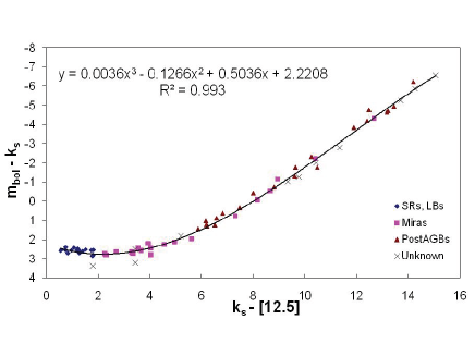
Figure 1: Bolometric correction exploited to determine the apparent magnitudes. See text for details.

In Section 2 we describe the methods adopted to build up our Carbon stars sample; updated Bolometric Corrections are presented in Section 3; the new LFGCS is shown and discussed in Section 4. Our conclusions follow in Section 5.

2 C-stars sample

In a previous paper, Guandalini et al. (2006) presented the observational LFGCS by collecting a sample of already published Carbon-rich AGB stars of the Milky Way. In that work, the sample was mainly made of stars that had mass loss estimates and for which distance estimates and/or mid-IR photometry were available.
Distance estimates were mainly taken from (in order of priority):

1. Bergeat & Chevallier 2005 (who re-analysed data from the original Hipparcos release);

2. Groenewegen et al. 2002;

3. Schöier & Olofsson 2001 and Loup et al. 1993.

Near-IR data were retrieved from the ground-based 2MASS survey (Cutri et al., 2003). Mid-IR photometry was taken from space telescopes ISO (SWS), MSX and IRAS (LRS). Selection criteria adopted to build up the sample have been (in order of priority):

• sources with ISO-SWS photometry;

• sources with enough mid-IR photometric data to apply Bolometric Corrections;

• application of the P-L relation for Mira variable sources from various references that are shown in the Tables of Guandalini et al. (2006).

The sample presented in Guandalini et al. (2006) consists of 230 sources (see their Fig. 8).

In recent years updated distance estimates for Galactic stars have become available, thanks to a release of revised Hipparcos astrometric data (van Leeuwen, 2007). Moreover, a new P-L relation for C-stars has been published by Whitelock et al. (2006). We construct a new LFGCS starting from the sample of Guandalini et al. (2006), by using the aforementioned upgrades and by following more stringent selection criteria, i.e.:

1. We keep in the sample only sources with distances derived from van Leeuwen (2007), selecting stars whose uncertainty in parallaxes is lower than half the parallax value. These sources must have ISO-SWS photometry or, on second option, photometric observations at mid-IR wavelengths that allow the application of the Bolometric Corrections (hereafter BC). These sources belong to different variability classes (i.e. Semiregulars and Miras).

2. If distances from Hipparcos are not available, we include the sources for which we can use the P-L relation presented by Whitelock et al. (2006) to directly determine the bolometric magnitude ($M_{bol}$) of the star, even if this relation has been derived for LMC sources. Feast et al. (2006) demonstrated that both the slope and the zero-point of the P-L relation for Galactic Carbon stars are similar to those derived for LMC Carbon stars. We therefore decided to adopt the P-L relation for LMC sources given in Whitelock et al. (2006) and thus we follow their suggestion (Feast et al., 2006). This relation has been applied to ”bona-fide” Mira-type stars only, thus excluding from the sample variable stars whose classification is uncertain. This approach implies notable changes with respect to the method adopted in Guandalini et al. (2006), who determined $M_{bol}$ by coupling their photometric analysis with distances determined from Period-Luminosity relations presented in various works [references shown in the Tables of Guandalini et al. (2006)]. However, the published P-L relations were obtained by calculating the apparent magnitude ($m_{bol}$) without considering mid-IR data (wavelengths larger than 8 $\mu$m), whose contribution for Carbon stars (and in particular for Mira variables) cannot be neglected. On the other hand, Guandalini et al. (2006) properly determined $m_{bol}$ analyzing the spectrum at least up to 12 $\mu$m (MSX, IRAS-LRS) and, when available, up to 45 $\mu$m (ISO-SWS). Thus, these distances could be overestimated, leading to an overestimation of $M_{bol}$ (up to half magnitude). Our procedure does not fix the need of mid-IR data, but, with respect to Guandalini et al. (2006), minimize the uncertainties in the analysis).

3. We exclude from the sample sources that seem to have a ”reliable” estimate of the distance from van Leeuwen (2007), but have estimates of the absolute bolometric magnitude fainter than $-3.5$. In fact, these stars cannot be AGB stars, but they could be Giants belonging to a binary system polluted by an already extinct AGB companion.

4. Unlike Guandalini et al. (2006), we exclude from the sample CJ stars and C(R) stars (due to the elusive nature of these objects; see e.g. Abia & Isern 2000; Piersanti et al. 2010).

5. We add to the sample sources from Whitelock et al. (2006); Le Bertre et al. (2005) not included in Guandalini et al. (2006) that follow the previous criteria.

The new sample consists of 102 sources, 32 stars exploiting distances from van Leeuwen 2007 and the remaining 70 from the PL-relation method. There are 72 Miras and 30 of other variability types (see the Online material for a list of the considered objects and their properties). With respect to Guandalini et al. (2006), the number of C-stars is greatly reduced (more than halved), but we reckon that the sample robustness is definitely improved. In fact, our sample contains both dust enshrouded stars (i.e. stars with high mass-loss rates, see Guandalini et al. 2006) and optically bright stars.

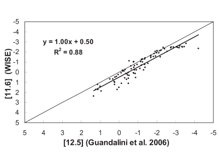
Figure 2: Comparison between the apparent magnitudes obtained by WISE at 11.6 $\mu$m and the ones used by us at 12.5 $\mu$m for the sources in our sample.

We also verified if the two adopted methods offer us comparable results. There are 5 Mira-type sources for which we have both a reliable estimate of the distance from Hipparcos and an estimate of the period of variability. Unfortunately, the catalogues we use do not have mid-IR data for two of them (U Cyg and RZ Peg). Notwithstanding, we exploit the photometric data from the recently released WISE catalogue (Cutri et al., 2012), in particular the fluxes for the filter centered at 11.6 $\mu$m. Note that our analysis exploits a different filter centered at 12.5 $\mu$m (TIRCAM - see Busso et al., 2007). We compare the fluxes obtained for the stars of our sample in these two photometric filters by WISE and by the catalogues used in this paper. In Fig.2 we observe a good correlation between the two sets of observations, with the ones in the 12.5 $\mu$m band on average 0.5 mag brighter than the ones in the 11.6 $\mu$m band. Therefore, we convert the WISE data at 11.6 $\mu$m according to the equation:

$$[11.6]_{WISE}=[12.5]_{G2006}+0.50$$ (1)

Hereafter we report our analysis for the 5 stars for which distance estimates from both the Hipparcos’ catalogue and the P-L relation are available:

1. R Lep: bolometric magnitude obtained thanks to mid-IR data and Hipparcos’ distance is $-$5.48, while if we take advantage of WISE data for mid-IR we obtain a bolometric magnitude of $-$5.55. The estimate obtained with the P-L method is $-$4.81 (around half magnitude fainter).

2. S Cep: bolometric magnitude obtained thanks to mid-IR data and Hipparcos’ distance is $-$5.42, while if we exploit WISE data for mid-IR we obtain a bolometric magnitude of $-$5.37. The estimate obtained with the P-L method is $-$4.96 (around half magnitude fainter).

3. U Cyg: bolometric magnitude obtained thanks to WISE data for mid-IR data and Hipparcos distance is $-$5.40. The estimate obtained with the P-L method is $-$4.90 (around half magnitude fainter).

4. V Oph: bolometric magnitude obtained thanks to mid-IR data and Hipparcos’ distance is $-$2.42, while if we use WISE data for mid-IR we obtain a bolometric magnitude of $-$2.42. The estimate obtained with the P-L method is $-$4.41.

5. RZ Peg: bolometric magnitude obtained thanks to WISE data for mid-IR data and Hipparcos distance is $-$1.69. The estimate obtained with the P-L method is $-$4.84.

The large differences in the last two sources (V Oph and RZ Peg) could be due to unreliable estimates of the distance from the Hipparcos’ catalogue. For these stars we adopt the estimate given by the P-L method, otherwise their luminosity would be inconsistent with those characterizing AGB stars.

The three remaining sources show that the P-L method give bolometric magnitudes around half magnitude fainter than the estimates obtained with mid-IR photometry and Hipparcos distances. The sample for which we can apply both methods is very small, therefore this comparison cannot give us clear indications about possible systematic biases between the two methods adopted in this analysis. Moreover, we note that there may be some objects in the sample with substantial errors in $M_{bol}$.
We found that the estimates of the absolute luminosity obtained taking advantage of the WISE data are very similar to the ones obtained adopting other mid-IR catalogues: in the study of the LF we are going to use WISE mid-IR photometry for R Lep, S Cep and U Cyg. The analysis of AGB stars of different chemical types with the WISE catalogue will be subject of a future paper.

3 Bolometric Corrections

In order to properly determine the apparent magnitude of our objects, we calculate again their BCs. In doing it, we consider a larger sample with respect to the one determined to construct the LFGCS. In particular, we analyze a large sample of intrinsic Carbon stars observed by ISO-SWS, without assuming as a constraint the distance estimate (note that the distance is not needed to estimate the BC of a stellar object), in order to obtain their $m_{bol}$. We adopt as a photometric index $m_{bol}-K_{s}$ (see Figure 1). Thus, as a by-product of our analysis, we produce a new BC, which represent another important improvement from to the ones presented in Guandalini et al. (2006) (see their Fig. 5).The BC presents a smaller peak value than the one obtained in Guandalini et al. (2006), even if we followed the same procedure to derive it. This is probably a consequence of using a different sample with respect to Guandalini et al. (2006).

4 The new Luminosity Function

In Fig. 3 we show the LFGCS derived in this paper (black solid line) and the one extracted from the C-stars sample analyzed by Guandalini et al. 2006 (red dashed line). The updated observational LFGCS confirms the behavior of the previous one at low and intermediate luminosities, with appreciable numbers starting at $M_{bol}\sim-4$ and the peak placed around $M_{bol}=-4.9$. The average uncertainty in the determination of $M_{bol}$ is around $\pm 0.3$ (see Whitelock et al. 2008). The main difference between the new and the old observational LFGCS consists in the high luminosity tail. In fact, the new LFGCS is truncated at $M_{bol}=-5.5$, and the high luminosity tail practically disappears. The absence of the high luminosity tail in the new LFGCS derives from the use of the aforementioned recent data and from new selection criteria. Thus, we demonstrate that the revised version of the Hipparcos catalogue (van Leeuwen, 2007) and a different choice in the exploitation of the P-L relations lead to significant changes in the derived LFGCS.

The new LFGCS is in agreement with extant theoretical studies (Cristallo et al., 2011) as shown in Fig.4. The theoretical LFGCS has been constructed by evaluating the contributions from all Galactic stars with different masses, ages and metallicities currently evolving along the AGB. The lower and upper mass on the AGB are estimated by interpolating the physical inputs (main sequence lifetime, AGB lifetime, bolometric magnitudes along the AGB) on the grid of computed models (M${}_{min}<$M/M${}_{\odot}<3.0$ M_⊙, with M_min depending on the metallicity). The theoretical LFGCS is nearly independent from the assumed Star Formation Rate, Initial Mass Function and metallicity distribution (see Cristallo et al. 2011 for details). The agreement between observational and theoretical LFGCS supports the validity of the adopted stellar models, whose intrinsic uncertainties (in particular the treatment of convection and the mass-loss history) restrain their predictive power.

We remark, however, that major uncertainties still affect the observational Luminosity Function of Galactic Carbon Stars. A giant step toward a better comprehension of Galactic C-stars and, thus, to the associated Luminosity Function, will be possible with the data from the GAIA mission. In fact, GAIA will produce, with an unprecedent precision, distance estimates for hundreds of thousands of Galactic C-stars (Eyer et al., 2012). Moreover, its continuous sky mapping over the mission time (an average of 70 measurements per object is currently planned) will provide more stringent constraints on the Period-Luminosity relations characterizing Mira and Semi-Regular variable stars. Moreover, we remind that the P-L relation was derived by Whitelock et al. (2006) exploiting only observation at near-IR wavelengths: a revision of the P-L relations considering also mid-IR photometry is needed. This further improvement will be possible only when dedicated surveys will release mid-IR data for Galactic and LMC Miras.

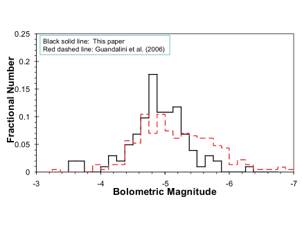
Figure 3: The Observational Luminosity Function of Galactic Carbon Stars derived in this paper (black solid line) compared with the Observational Luminosity Function of Galactic Carbon Stars presented by Guandalini et al. 2006 (red dashed line).

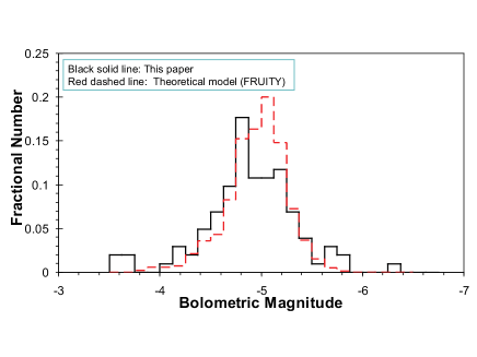
Figure 4: The Observational Luminosity Function of Galactic Carbon Stars derived in this paper (black solid line), compared with the theoretical LFGCS published by Cristallo et al. 2011 (red dashed line).

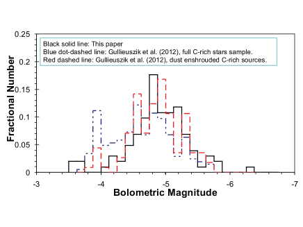
Figure 5: The Observational Luminosity Function of Galactic Carbon Stars derived in this paper (black solid line), compared with the Luminosity Function of Carbon Stars in the Large Magellanic Cloud presented by Gullieuszik et al. 2012 for the entire C-rich sample (blue dot-dashed line) and for the sub-sample of the dust-enshrouded sources (red dashed line).

The problem of the distance determination does not affect the Luminosity Function of Carbon Stars in the Large Magellanic Cloud, since all C-stars belonging to that system can be considered at a fixed distance with only moderate depth. Thus, any difference in $m_{bol}$ implies a rescaled difference in luminosity. In Figure 5 we report the Luminosity Function of Carbon stars in LMC derived by Gullieuszik et al. (2012). We note that the Luminosity Function, as obtained from their full sample (dot-dashed curve), is more weighted toward fainter $M_{bol}$ than our LFGCS. We should note, however, that the same authors claimed a possible misclassification of faint C-rich stars. Moreover, the sample presented by Gullieuszik et al. (2012) also contains C(J) stars, while our LFGCS only contains C(N) stars, i.e. AGB stars currently experiencing Third Dredge Up episodes. It is worth to remind that the origin of C(J) stars is still unknown and that a considerable percentage of these stars show infrared emission associated with silicate dust (see e.g. Hedrosa et al. 2013), while amorphous carbon is expected to dominate the atmospheres of C(N) stars. Thus, we suspect that C(J) stars could be classified as dust-free in the sample of Gullieuszik et al. (2012). Considering the aforementioned problems, we reckon that the right sample to be compared with our LFGCS is the dusty one presented by Gullieuszik et al. 2012 (see their Figure 6). For this reason, in Figure 5 we also report this sub-sample (dashed curve). The latter (see also Cohen et al. 1981) peaks at the same Bolometric Magnitude and presents a shape very similar to the LFGCS presented in this paper.

This seems to suggest that, for intermediate and large metallicities, the Luminosity Function of Carbon Stars weakly depends on the initial metal content and that its magnitude range is nearly the same ($-4.5<M_{bol}<-5.5$). The main difference between the two Luminosity Functions shown in Fig. 5 is a very small shift to lower luminosities for the sources of the Large Magellanic Cloud. This fact is expected from theoretical calculations (see Cristallo et al. 2011, in particular their Fig. 11). At lower metallicities, in fact, the reduced oxygen content makes the carbon phase (C/O¿1) on the AGB easier to be reached at lower luminosities (in earlier evolutionary stages). Moreover, the enhanced TDU efficiency and the larger contribution from lower masses (see Cristallo et al. 2009) further weight the Luminosity Function of Carbon Stars to lower luminosities. New observations of Carbon Stars in low metallicity environments, such as the Small Magellanic Cloud and Dwarf galaxies (see Sloan et al. 2012 and references therein), could further shed light on this problem. This analysis, however, is beyond the scope of this paper.

Table 1: Sample used to estimate the Luminosity Function.

Source	Var. Type	Distance (Kpc)	Period (days)	Absolute
name	(GCVS)	(van Leeuwen, 2007)	(GCVS)	Magnitude
W Cas	Mira	$-$	405.57	$-$4.75
HV Cas	Mira	$-$	527	$-$5.04
X Cas	Mira	$-$	422.84	$-$4.80
YY Tri	Mira	$-$	624	$-$5.23
R For	Mira	$-$	388.73	$-$4.71
V384 Per	Mira	$-$	535	$-$5.06
V718 Tau	Mira	$-$	405	$-$4.75
AU Aur	Mira	$-$	400.5	$-$4.74
R Ori	Mira	$-$	377.1	$-$4.67
R Lep	Mira	0.47	427.07	$-$5.55
NAME SHV F4488	Mira	$-$	573	$-$5.14
WBP 14	Mira	$-$	325	$-$4.51
V370 Aur	Mira	$-$	683	$-$5.33
QS Ori	Mira	$-$	476	$-$4.93
V617 Mon	Mira	$-$	375	$-$4.67
ZZ Gem	Mira	$-$	317	$-$4.48
V636 Mon	Mira	$-$	543	$-$5.08
V503 Mon	Mira	$-$	355	$-$4.61
RT Gem	Mira	$-$	350.4	$-$4.59
CG Mon	Mira	$-$	419.11	$-$4.79
CL Mon	Mira	$-$	497.15	$-$4.98
R Vol	Mira	$-$	453.6	$-$4.88
HX CMa	Mira	$-$	725	$-$5.40
VX Gem	Mira	$-$	379.4	$-$4.68
V831 Mon	Mira	$-$	319	$-$4.49
V346 Pup	Mira	$-$	571	$-$5.13
FF Pup	Mira	$-$	436	$-$4.83
IQ Hya	Mira	$-$	397	$-$4.73
CQ Pyx	Mira	$-$	659	$-$5.29
CW Leo	Mira	$-$	630	$-$5.24
CZ Hya	Mira	$-$	442	$-$4.85
TU Car	Mira	$-$	258	$-$4.26
FU Car	Mira	$-$	365	$-$4.64
V354 Cen	Mira	$-$	150.4	$-$3.66
BH Cru	Mira	$-$	421	$-$4.80
V1132 Cen	Mira	$-$	560	$-$5.11
V Cru	Mira	$-$	376.5	$-$4.67
TT Cen	Mira	$-$	462	$-$4.90
RV Cen	Mira	$-$	446	$-$4.86
II Lup	Mira	$-$	580	$-$5.15
V CrB	Mira	$-$	357.63	$-$4.62
NP Her	Mira	$-$	448	$-$4.86
V Oph	Mira	0.24	297.21	$-$4.41
V2548 Oph	Mira	$-$	747	$-$5.43
V617 Sco	Mira	$-$	523.6	$-$5.04
V833 Her	Mira	$-$	540	$-$5.07
T Dra	Mira	$-$	421.62	$-$4.80
V1280 Sgr	Mira	$-$	523	$-$5.03
V5104 Sgr	Mira	$-$	655	$-$5.28
V1076 Her	Mira	$-$	609	$-$5.20
V627 Oph	Mira	$-$	452	$-$4.87
V821 Her	Mira	$-$	511	$-$5.01
V1417 Aql	Mira	$-$	617	$-$5.22
V874 Aql	Mira	$-$	145	$-$3.62
V2045 Sgr	Mira	$-$	451	$-$4.87
AI Sct	Mira	$-$	408	$-$4.76
V1420 Aql	Mira	$-$	676	$-$5.32
V1965 Cyg	Mira	$-$	625	$-$5.23
KL Cyg	Mira	$-$	526	$-$5.04
R Cap	Mira	$-$	345.13	$-$4.58
U Cyg	Mira	0.52	463.24	$-$5.40
BD Vul	Mira	$-$	430	$-$4.82
V Cyg	Mira	$-$	421.27	$-$4.80
V442 Vul	Mira	$-$	661	$-$5.29
RV Aqr	Mira	$-$	453	$-$4.88
V1426 Cyg	Mira	$-$	470	$-$4.92
S Cep	Mira	0.41	486.84	$-$5.37
V1568 Cyg	Mira	$-$	495	$-$4.97
RZ Peg	Mira	0.21	438.7	$-$4.84
LL Peg	Mira	$-$	696	$-$5.35
IZ Peg	Mira	$-$	486	$-$4.95
LP And	Mira	$-$	614	$-$5.21
VX And	SRA	0.39	375	$-$4.16
Z Psc	SRB	0.38	144	$-$4.40
R Scl	SRB	0.27	370	$-$3.71
TW Hor	SRB	0.32	158	$-$4.62
TT Tau	SRB	0.36	166.5	$-$4.24
W Ori	SRB	0.38	212	$-$5.76
W Pic	LB	0.78	$-$	$-$5.73
Y Tau	SRB	0.36	241.5	$-$4.70
NP Pup	LB	0.50	$-$	$-$5.02
X Cnc	SRB	0.34	195	$-$4.96
Y Hya	SRB	0.39	302.8	$-$4.76
X Vel	SR	0.36	140	$-$4.51
U Ant	LB	0.27	$-$	$-$5.22
VY UMa	LB	0.38	$-$	$-$4.75
V996 Cen	LB	0.64	$-$	$-$5.48
X TrA	LB	0.36	$-$	$-$5.74
V Pav	SRB	0.37	225.4	$-$4.91
S Sct	SRB	0.39	148	$-$4.73
V Aql	SRB	0.36	353	$-$5.19
UX Dra	SRA	0.39	168	$-$4.90
AQ Sgr	SRB	0.33	199.6	$-$4.11
TT Cyg	SRB	0.56	118	$-$4.22
AX Cyg	LB	0.37	$-$	$-$3.60
T Ind	SRB	0.58	320	$-$5.86
Y Pav	SRB	0.40	233.3	$-$5.11
V460 Cyg	SRB	0.62	180	$-$6.28
TX Psc	LB	0.28	$-$	$-$5.15
UY Cen	SR	0.67	114.6	$-$5.73
RX Sct	LB	0.43	$-$	$-$4.29
RS Cyg	SRA	0.47	417.39	$-$4.39

Table 1: continued.

5 Conclusions

In this paper we present a revised observational LFGCS. New available data (revised Hipparcos distances from van Leeuwen 2007 and Period-Luminosity relations from Whitelock et al. 2006) and more stringent criteria have been adopted to select the C-star sample. We confirm the LFGCS of Guandalini et al. (2006) at low and intermediate luminosities. On the contrary, at high luminosities the new LFGCS is abruptly truncated at $M_{bol}=-5.5$, in agreement with extant theoretical studies (Cristallo et al., 2011). The disappearance of the high luminosity tail derives from the use of the aforementioned recent data and new selection criteria.

The Luminosity Functions of dusty Carbon Stars in the Large Magellanic Cloud (see Gullieuszik et al. 2012 for a recent derivation) peaks at the same Bolometric Magnitude with respect to its Galactic counterpart, presenting a very similar shape. This seems to suggest that the Luminosity Functions of Carbon Stars slightly depends on the initial metal content and that its magnitude range is nearly the same ($-4.5<M_{bol}<-5.5$) in stellar systems with intermediate and large metallicities, as suggested by Cristallo et al. (2011). Observations are well reproduced by AGB theoretical models. This demonstrates the goodness in the choice of critical parameters affecting their evolution, such as the treatment of convection or the mass-loss history, whose complex interplay determines the duration and the luminosity of the C-rich phase.