Quickest Change Point Detection and Identification Across a Generic Sensor Array

Abstract

In this paper, we consider the problem of quickest change point detection and identification over a linear array of $N$ sensors, where the change pattern could first reach any of these sensors, and then propagate to the other sensors. Our goal is not only to detect the presence of such a change as quickly as possible, but also to identify which sensor that the change pattern first reaches. We jointly design two decision rules: a stopping rule, which determines when we should stop sampling and claim a change occurred, and a terminal decision rule, which decides which sensor that the change pattern reaches first, with the objective to strike a balance among the detection delay, the false alarm probability, and the false identification probability. We show that this problem can be converted to a Markov optimal stopping time problem, from which some technical tools could be borrowed. Furthermore, to avoid the high implementation complexity issue of the optimal rules, we develop a scheme with a much simpler structure and certain performance guarantee.

I Introduction

The standard quickest change detection problem is set to detect some unknown time point at which certain signal probability distribution changes over a sequence of observations. Recently, with the development of wireless sensor networks, multiple sensors can be deployed to execute the quickest change detection, and the sensors can send quantized or unquantized observations or certain local decisions to a control center, who then makes a final decision [1, 2]. Most of the existing work is based on an assumption that the statistical properties of observations at all sensors change simultaneously. However, in certain scenarios, this assumption may not hold well. For instance, when multiple sensors are used to detect the occurrence of the chemical leakage, the sensors that are closer to the leakage source usually observe the change earlier than those far away from the source. In such cases, two interesting problems arise: one is to detect the change as soon as possible; the other is to identify which sensor is the closest to the source, such that we could have a first-order inference over the leakage source location.

As far as we know, currently there are few work studying the case of change occurring non-simultaneously. In the related work, the authors in [3] proposed a scheme that each sensor makes a local decision with the computing burden at the local sensors, where they did not consider the identification problem. In [4], the authors modeled the change propagation process as a Markov process to derive the optimal stopping rule and assumed that the change pattern always first reaches a predetermined sensor, such that the identification problem is ignored. In [5], the identification problem for the special case of two sensors was studied, where the sufficient statistic is proven as a Markov process and a joint optimal stopping rule and terminal decision rule are proposed.

In this paper, we study the joint change point detection and identification problem over a linear array of $N$ sensors, where the change first occurs near an unknown sensor, then propagates to sensors further away. We assume that all sensors send their observations to a control center. With the sequential observation signals, the control center first operates a stopping rule to decide when to alarm that the change has occurred; then the control center deploys a terminal decision rule to determine which sensor that the change pattern reaches first. In our setup, three performance metrics are of interest: i) detection delay, which is the time interval between the moment that the change occurs and the moment that an alarm is raised; ii) false alarm probability, which is the probability that an alarm is raised before the actual change occurs; and iii) false identification probability, which is the probability that the control center does not correctly identify the sensor that the change pattern first reaches. We apply the Markov optimal stopping time theory to design the optimal decision rules to minimize a weighted sum of the above three metrics. Furthermore, we derive a scheme with a much simpler structure and certain performance guarantee.

The rest of this paper is organized as follows. In Section II, we introduce the system model. In Section III, we derive the optimal decision rules. In Section IV, we propose a scheme approximate to the optimal decision rules with a much lower complexity. In Section V, we present some numerical results, with conclusions in Section VI.

II System Model

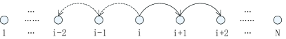
Figure 1: A sensor array with $S=i$

We consider a scenario with $N$ sensors constructing a linear array to monitor the environment, as shown in Fig. 1. At an unknown time point, a change occurs at an unknown location and propagates, where we use change point time $\Gamma_{i}$ to denote the time that the change pattern reaches sensor $i$. We further use $S$ to denote the index of the sensor that the change pattern first reaches. We focus on the Bayesian setup and use $p_{i}$ to denote the prior probability of $\{S=i\}$, simply with $p_{i}=1/N$. Conditioned on the event that the change pattern first reaches sensor $i$, $\Gamma_{i}$ is assumed to bear a geometric distribution [4, 5] with parameter $\rho$, $0<\rho\leq 1$ i.e.,

$$P[\Gamma_{i}=k|S=i]=\rho(1-\rho)^{k},k\geq 0,$$ (1)

where $k$ denotes the discretized time and takes integer values.

We consider the practical factors in the environment, such as the wind or the blockers, which will affect the propagation speed of the change. For instance, see in Fig. 1, if the direction of the wind is from the left to the right side in the monitored scenario, then the propagation of the air pollution will be much faster at the right side of sensor $S=i$ than that of the left side. And at the same side, the propagation follows the deterministic order shown as

$$\left\{\begin{array}[]{l}i\to i-1\to i-2\to i-3......\\ i\to i+1\to i+2\to i+3......\\ \end{array}\right.$$ (2)

We further assume that after the change patten reaches the first sensor $i$, for the right side of sensor $i$, it will propagate from one sensor to another sensor following the geometric propagation models as

$$P[\Gamma_{j+1}=k_{1}+k_{2}|\Gamma_{j}=k_{1},S=i]=\rho_{1}(1-\rho_{1})^{k_{2}},j>i,k_{2}\geq 0,$$ (3)

while for the left side of sensor $i$, the propagation follows

$$P[\Gamma_{j-1}=k_{1}+k_{2}|\Gamma_{j}=k_{1},S=i]=\rho_{2}(1-\rho_{2})^{k_{2}},j<i,k_{2}\geq 0,$$ (4)

where $\rho_{1}$ and $\rho_{2}$ are used to model possibly different propagation speed along each direction, e.g., $\rho_{1}>\rho_{2}$ means the propagation speed is higher at the right side that that of the left side.

Taking above assumption, for $S=i$, we define all possible $i\times(N-i+1)+1$ events at time $k$ as follows:

$$\begin{array}[]{l}T_{0,k}=\{{\Gamma_{i}}>k,{\Gamma_{i-1}}>k,{\Gamma_{i+1}}>k,{\Gamma_{i-2}}>k,{\Gamma_{i+2}}>k,...\}\\ T_{1,k}=\{{\Gamma_{i}}\leq k,{\Gamma_{i-1}}>k,{\Gamma_{i+1}}>k,{\Gamma_{i-2}}>k,{\Gamma_{i+2}}>k,...\}\\ T_{2,k}=\{{\Gamma_{i}}\leq k,{\Gamma_{i-1}}>k,{\Gamma_{i+1}}\leq k,{\Gamma_{i-2}}>k,{\Gamma_{i+2}}>k,...\}\\ T_{3,k}=\{{\Gamma_{i}}\leq k,{\Gamma_{i-1}}>k,{\Gamma_{i+1}}\leq k,{\Gamma_{i-2}}>k,{\Gamma_{i+2}}\leq k,...\}\\ \vdots\\ T_{N-i+1,k}=\{{\Gamma_{i}}\leq k,{\Gamma_{i-1}}>k,{\Gamma_{i+1}}\leq k,...,{\Gamma_{N}}\leq k\}\\ T_{N-i+2,k}=\{{\Gamma_{i}}\leq k,{\Gamma_{i-1}}\leq k,{\Gamma_{i+1}}>k,{\Gamma_{i-2}}>k,{\Gamma_{i+2}}>k,...\}\\ T_{N-i+3,k}=\{{\Gamma_{i}}\leq k,{\Gamma_{i-1}}\leq k,{\Gamma_{i+1}}\leq k,{\Gamma_{i-2}}>k,{\Gamma_{i+2}}>k,...\}\\ T_{N-i+4,k}=\{{\Gamma_{i}}\leq k,{\Gamma_{i-1}}\leq k,{\Gamma_{i+1}}\leq k,{\Gamma_{i-2}}>k,{\Gamma_{i+2}}\leq k,...\}\\ \vdots\\ T_{2(N-i+1),k}=\{{\Gamma_{i}}\leq k,{\Gamma_{i-1}}\leq k,{\Gamma_{i+1}}\leq k,...,{\Gamma_{N}}\leq k\}\\ \vdots\\ T_{(i-1)(N-i+1)+1,k}=\{{\Gamma_{i}}\leq k,{\Gamma_{i-1}}\leq k,{\Gamma_{i+1}}>k,...,{\Gamma_{1}}\leq k\}\\ \vdots\\ T_{i(N-i+1),k}=\{{\Gamma_{i}}\leq k,{\Gamma_{i-1}}\leq k,{\Gamma_{i+1}}\leq k,...,{\Gamma_{1}}\leq k,{\Gamma_{N}}\leq k\},\end{array}$$

where $T_{1,k}\sim T_{N-i+1,k}$ denote the events that after the change pattern first reaching sensor $i$, it propagates across the sensors sequentially at the right side of sensor $i$. The number of events equals to the number of sensors at the right side plus 1, i.e., $N-i+1$. $T_{N-i+2,k}\sim T_{2(N-i+1),k}$ denote the events that after the change pattern reaching sensor $i$ and $i-1$, it propagates across the sensors sequentially at the right side of sensor $i$, and the number of events is also $N-i+1$, which is the same for the case that after the change pattern reaching sensor $i$, $i-1$, $i-2$ and so on. Since there are $i-1$ sensors at the left side of sensor $i$ and the event of no change pattern reaches any sensor is $T_{0,k}$, the total number of possible events is $i\times(N-i+1)+1$.

At each time $k$, we assume that the observations ${{\bf{z}}_{k}}=[{{{z}}_{1,k}},...,{{{z}}_{N,k}}]$ from all sensors are available at a control center. For each sensor $i$, conditioned on $\Gamma_{i}$, ${{z}}_{i,k}$ is Identically and Independently Distributed (IID) according to $f_{0}$ before $\Gamma_{i}$, and IID according to $f_{1}$ after $\Gamma_{i}$, i.e.,

$$z_{i,k}\sim\begin{cases}&f_{0},~{}~{}~{}~{}k<\Gamma_{i},\\ &f_{1},~{}~{}~{}~{}k\geq\Gamma_{i}.\end{cases}$$ (5)

The observation sequence $\{\mathbf{z}_{k};k=1,2,...\}$ generates a filtration $\{\mathcal{F}_{k};k=1,2,...\}$ with

$${{\cal F}_{k}}=\sigma({{\bf{z}}_{1}},...,{{\bf{z}}_{k}},\{\Gamma=0\}),k=1,2,...$$ (6)

where $\sigma({{\bf{z}}_{1}},...,{{\bf{z}}_{k}},\{\Gamma=0\})$ denotes the smallest $\sigma$-field in which $({{\bf{z}}_{1}},...,{{\bf{z}}_{k}},\{\Gamma=0\})$ is measurable and $\Gamma=\min\{\Gamma_{1},...,\Gamma_{N}\}$.

We use $P$ to denote the probability measure that specifies the prior distribution of $\{S=i\}$, the distribution of change point time, and the distribution of $\{\mathbf{z}_{k};k=1,2,...\}$. We also use $\mathbb{E}$ to denote the expectation under the probability measure $P$. Specifically, we use $P_{i}$ to denote the probability measure when $S=i$.

With above setups, the control center needs to detect the earliest change point time $\Gamma=\min\{\Gamma_{1},...,\Gamma_{N}\}$ as soon as it occurs. A stopping time $\tau$ will be decided for when to stop sampling and alarm that a change has occurred, where a false alarm may happen if $\tau<\Gamma$. We target to minimize the averaged detection delay $\mathbb{E}\{(\tau-\Gamma)^{+}\}$ with keeping the false alarm probability $P[\tau<\Gamma]$ small. In addition, we also require the control center to identify which sensor the change pattern reaches first. We adopt $\delta_{k}$ to denote the $\mathcal{F}_{k}$-measurable terminal decision rule used by the control center to make the identification, and $\hat{S}$ to denote the index of the sensor identified, i.e., $\hat{S}=\delta_{k}(\mathcal{F}_{k})$. A false identification occurs if $\hat{S}\neq S$, such that we also want to keep $P[\hat{S}\neq S]$ small. We use $\boldsymbol{\delta}=\{\delta_{1},\delta_{2},...\}$ to denote the sequence of terminal decision rules. Summarizing above, our goal is to design a stopping time $\tau$ and a terminal decision rule $\boldsymbol{\delta}$ that minimize the aggregated risk function defined as

$$R\triangleq P[\tau<\Gamma]+c_{1}\mathbb{E}\{(\tau-\Gamma)^{+}\}+c_{2}P[\hat{B}_{1}\neq B_{1}],$$ (7)

where $c_{1}$ and $c_{2}$ are appropriate constants that balance the three costs.

III Optimal Rules

In this section, we present the optimal stopping and terminal decision rules. To proceed, we define the following posterior probabilities at time $k$:

$${\pi_{j,k\left|i\right.}}=P[T_{j,k}\left|{{{\cal F}_{k}},S=i}\right.],~{}i=1,...,N,~{}j=0,...,i(N-i+1),$$ (8)

$$p_{k}^{i}=P[{S}=i\left|{{{\cal F}_{k}}}\right.],~{}i=1,...,N.$$ (9)

We also define the following matrices and vectors:

$${{\boldsymbol{\pi}}_{k}}={[{\pi_{j,k\left|i\right.}}]_{M\times N}},$$ (10)

$${\bf{p}}_{k}=[p_{k}^{1},p_{k}^{2},...,p_{k}^{N}]_{1\times N},$$ (11)

where $M=(N-\lfloor\frac{N+1}{2}\rfloor+1)\times\lfloor\frac{N+1}{2}\rfloor+1$ denotes the maximum number of events defined in Section II for $i\in\{1,...,N\}$. Corresponding to $M$, $i=\lfloor\frac{N+1}{2}\rfloor$. For each $i$ with the number of events less than $M$, the extra elements in ${\boldsymbol{\pi}}_{k}$ are set as 0.

With the posterior probabilities defined above, we denote $\mathbf{q}_{k}=\{{\boldsymbol{\pi}}_{k},{\bf{p}}_{k}\}$.

We first have the following theorem regarding the optimal terminal decision rule $\boldsymbol{\delta}$.

Theorem 1

For any stopping time $\tau$, the optimal terminal decision rule is

$$\hat{S}=\arg\max\limits_{1\leq i\leq N}\left\{p_{\tau}^{1},...,p_{\tau}^{i},...,p_{\tau}^{N}\right\},$$ (12)

and we have

$$\inf\limits_{\boldsymbol{\delta}}P[\hat{S}\neq S]=\mathbb{E}\left\{1-\max\left\{p_{\tau}^{1},...,p_{\tau}^{N}\right\}\right\}.$$ (13)

The proof follows from Proposition 4.1 of [6]. Theorem 1 implies that the optimal terminal decision rule is simply to choose the sensor that has the largest posterior probability. A similar situation also arises in the multiple hypothesis testing problem considered in [7].

Using above optimal terminal decision rule, we can further express the optimization objective in (7) as a function of the posterior probabilities defined in (8) and (9), as shown below.

Lemma 1

For any stopping time $\tau$, (7) can be written as

$$\begin{split}R=\mathbb{E}&\left\{\sum\limits_{i=1}^{N}{{{\pi_{0,\tau\left|i\right.}}}}p_{\tau}^{i}+c_{2}\left(1-\max\left\{p_{\tau}^{1},...,p_{\tau}^{N}\right\}\right)\right.\\ &~{}~{}+\left.{c_{1}}\sum\limits_{k=0}^{\tau-1}{\left(1-\sum\limits_{i=1}^{N}{{\pi_{0,k\left|i\right.}}}p_{k}^{i}\right)}\right\}.\end{split}$$ (14)

Proof:

Based on the Bayesian’s rule, we have

$$P[\Gamma>k\left|{{{\cal F}_{k}}}\right.]=P[T_{0,k}\left|{{{\cal F}_{k}}}\right.] =\sum\limits_{i=1}^{N}{P[T_{0,k}\left|{{{\cal F}_{k}}}\right.,B=i]}p_{k}^{i}$$

$$=\sum\limits_{i=1}^{N}{{\pi_{0,k\left|i\right.}}}p_{k}^{i}.$$ (15)

Further, according to Proposition 5.1 in [6],

$$P[\tau<\Gamma]+c_{1}\mathbb{E}\{(\tau-\Gamma)^{+}\}$$

$$=\mathbb{E}\left\{P[\tau<\Gamma|\mathcal{F}_{\tau}]+c_{1}\sum\limits_{k=0}\limits^{\tau-1}P[\Gamma\leq k|\mathcal{F}_{k}]\right\}$$

$$=\mathbb{E}\left\{\sum\limits_{i=1}^{N}{{\pi_{0,\tau\left|i\right.}}}p_{\tau}^{i}+{c_{1}}\sum\limits_{k=0}^{\tau-1}\left(1-\sum\limits_{i=1}^{N}{{\pi_{0,k\left|i\right.}}}p_{k}^{i}\right)\right\}.$$ (16)

By combining (13), we complete the proof. ∎

Furthermore, we have the following lemma regarding $\mathbf{q}_{k}$.

Lemma 2

There is a time-invariant function $g$ such that $\mathbf{q}_{k}=g(\mathbf{q}_{k-1},\mathbf{z}_{k})$.

Proof:

We have

$$\pi_{j,k|i}=P[T_{j,k}|{\cal F}_{k-1},{{\bf{z}}_{k}},S=i]$$

$$=\frac{{f({{\bf{z}}_{k}}\left|{{{\cal F}_{k-1}},T_{j,k}}\right.,{S}=i)P[T_{j,k}\left|{{{\cal F}_{k-1}},S=i}\right.]}}{{\sum\limits_{j=0}^{i(N-i+1)}{f({{\bf{z}}_{k}}\left|{{{\cal F}_{k-1}},T_{j,k}}\right.,{S}=i)P[T_{j,k}\left|{{{\cal F}_{k-1}},S=i}\right.]}}},$$ (17)

in which

$$f({{\bf{z}}_{k}}\left|{{{\cal F}_{k-1}},T_{0,k}}\right.,S=i)={f_{0}}({z_{i,k}}){f_{0}}({z_{i-1,k}}){f_{0}}({z_{i+1,k}})......$$

$$f({{\bf{z}}_{k}}\left|{{{\cal F}_{k-1}},T_{1,k}}\right.,S=i)={f_{1}}({z_{i,k}}){f_{0}}({z_{i-1,k}}){f_{0}}({z_{i+1,k}})......$$

$${\rm{}}\vdots$$

$$f({{\bf{z}}_{k}}\left|{{{\cal F}_{k-1}},T_{i(N-i+1),k}}\right.,S=i)={f_{1}}({z_{i,k}}){f_{1}}({z_{i-1,k}}){f_{1}}({z_{i+1,k}})......$$

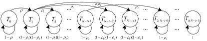
Figure 2: Transition probabilities

Since the geometric distribution based model owns the memoryless property, the transition probabilities of the events are shown in Fig. 2. According to these transition probabilities, we have

$$P[T_{0,k}|{{{\cal F}_{k-1}},S=i}]=(1-\rho)\pi_{0,{k-1}|i},$$

$$P[T_{1,k}|{{{\cal F}_{k-1}},S=i}]=(1-{\rho_{1}})(1-{\rho_{2}}){\pi_{1,k-1\left|{i}\right.}}+\rho{\pi_{0,k-1\left|{i}\right.}}$$

$${\rm{}}\vdots$$

$$P[T_{N-i+1,k}|{{{\cal F}_{k-1}},S=i}]=(1-{\rho_{2}}){\pi_{N-i+1,k-1\left|{i}\right.}}+\rho_{1}{\pi_{N-i,k-1\left|{i}\right.}}$$

$$P[T_{N-i+2,k}|{{{\cal F}_{k-1}},S=i}]=(1-{\rho_{1}})(1-{\rho_{2}}){\pi_{N-i+2,k-1\left|{i}\right.}}+\rho_{2}{\pi_{1,k-1\left|{i}\right.}}$$

$$P[T_{N-i+3,k}|{{{\cal F}_{k-1}},S=i}]=(1-{\rho_{1}})(1-{\rho_{2}}){\pi_{N-i+3,k-1\left|{i}\right.}}$$

$$~{}~{}~{}~{}~{}~{}~{}~{}~{}~{}~{}~{}~{}~{}~{}~{}~{}~{}~{}~{}~{}~{}~{}~{}~{}~{}~{}~{}+\rho_{1}{\pi_{N-i+2,k-1\left|{i}\right.}}+\rho_{2}{\pi_{2,k-1\left|{i}\right.}}+\rho_{1}\rho_{2}{\pi_{1,k-1\left|{i}\right.}}$$

$${\rm{}}\vdots$$ (19)

Therefore, $\boldsymbol{\pi}_{k}$ can be computed by $\mathbf{q}_{k-1}$ and $\mathbf{z}_{k}$.

For another element ${\bf{p}}_{k}$ in $\mathbf{q}_{k}$, we have

$$\begin{split}p_{k}^{i}&=P[{S}=i\left|{{{\cal F}_{k-1}},{{\bf{z}}_{k}}}\right.]\\ &=\frac{{f({{\bf{z}}_{k}}\left|{{{\cal F}_{k-1}},{S}=i}\right.)P[{S}=i\left|{{{\cal F}_{k-1}}}\right.]}}{{\sum\limits_{n=0}^{M-1}{f({{\bf{z}}_{k}}\left|{{{\cal F}_{k-1}},{S}=n}\right.)P[{S}=n\left|{{{\cal F}_{k-1}}}\right.]}}},\end{split}$$ (20)

where

$$f({{\bf{z}}_{k}}\left|{{{\cal F}_{k-1}},{S}=n}\right.)$$

$$=\sum\limits_{j=0}^{M-1}f({{\bf{z}}_{k}}\left|{{{\cal F}_{k-1}},T_{j,k}}\right.,S=n)P[T_{j,k}|{{{\cal F}_{k-1}},S=n}],$$ (21)

which can be calculated by using (III) and (III). Hence, ${\bf{p}}_{k}$ can also be computed by $\mathbf{q}_{k-1}$ and $\mathbf{z}_{k}$. ∎

This lemma implies that the posterior probabilities $\mathbf{q}_{k}$ can be recursively computed from $\mathbf{q}_{k-1}$ and $\mathbf{z}_{k}$. Combined with Lemma 1, we know that $\mathbf{q}_{k}$ is a sufficient statistic for the problem of minimizing (14). Thus, the problem at the hand is a Markov stopping time problem.

Therefore, we could borrow results from the optimal stopping time theory to design the optimal decision rules for our problem. We first consider a finite time horizon case, in which one has to make a decision before a deadline $T$, i.e., $\tau\leq T$. It is easy to check that the cost-to-go functions are

$$J_{T}^{T}(\mathbf{q}_{T})=\sum\limits_{i=1}^{N} {{\pi_{0,T\left|i\right.}}}p_{T}^{i}+c_{2}\left(1-\max\left\{p_{T}^{1},...,p_{T}^{N}\right\}\right),\texttt{and}$$

$$J_{k}^{T}(\mathbf{q}_{k})=\min \left\{{\sum\limits_{i=1}^{N}{{\pi_{0,k\left|i\right.}}}p_{k}^{i}}+c_{2}\left(1-\max\left\{p_{k}^{1},...,p_{k}^{N}\right\}\right),\right.$$

$$~{}~{}\left.c_{1}\left(1-\sum\limits_{i=1}^{N}{{\pi_{0,k\left|i\right.}}}p_{k}^{i}\right)+A_{k}^{T}(\mathbf{q}_{k})\right\},$$ (22)

where

$$A_{k}^{T}(\mathbf{q}_{k})=\mathbb{E}\left\{J_{k+1}^{T}(\mathbf{q}_{k+1})|\mathcal{F}_{k}\right\}=\int J_{k+1}^{T}(g(\mathbf{q}_{k},\mathbf{z}))f(\mathbf{z}|\mathcal{F}_{k})d\mathbf{z}.$$

Applying the optimal stopping time theory [6], we have the following theorem for the optimal decision rules.

Theorem 2

The optimal stopping time is obtained as

$$\tau_{opt}=\inf \left\{k:{\sum\limits_{i=1}^{N}{{\pi_{0,k\left|i\right.}}}p_{k}^{i}}+c_{2}\left(1-\max\left\{p_{k}^{1},...,p_{k}^{N}\right\}\right)\right.$$

$$~{}~{}~{}~{}~{}~{}~{}~{}\left.\leq c_{1}\left(1-\sum\limits_{i=1}^{N}{{\pi_{0,k\left|i\right.}}}p_{k}^{i}\right)+A_{k}^{T}(\mathbf{q}_{k})\right\},$$ (23)

with the optimal terminal decision rule is given in (12).

In the infinite time horizon case when $T\rightarrow\infty$, we have $J_{k}^{\infty}(\mathbf{q})$ defined as

$$J_{k}^{\infty}(\mathbf{q})=\lim_{T\rightarrow\infty}J_{k}^{T}(\mathbf{q}),$$ (24)

since we have $J_{k}^{T}(\mathbf{q})>0$, $J_{k}^{T+1}(\mathbf{q})\leq J_{k}^{T}(\mathbf{q})$, and the fact that all strategies allowed with deadline $T$ are also allowed with deadline $T+1$. Since the observations are memoryless and conditionally IID, $J_{k}^{\infty}(\mathbf{q})$ is the same for all $k$; we then use $J(\mathbf{q})$ to denote $J_{k}^{\infty}(\mathbf{q})$. Thus, $A(\mathbf{q})$ is derived as

$$\begin{split}A(\mathbf{q})=\lim_{T\rightarrow\infty}A_{k}^{T}(\mathbf{q})&=\int\lim_{T\rightarrow\infty}J_{k+1}^{T}(g(\mathbf{q},\mathbf{z}))f(\mathbf{z}|\mathbf{q})d\mathbf{z}\\ &=\int J(g(\mathbf{q},\mathbf{z}))f(\mathbf{z}|\mathbf{q})d\mathbf{z},\end{split}$$ (25)

in which the interchange of $\lim$ and $\int$ is allowed due to the dominated convergence theorem.

Therefore, when the deadline is infinite, the optimal stopping rule becomes

$$\tau_{opt}=\inf \left\{k:{\sum\limits_{i=1}^{N}{{\pi_{0,k\left|i\right.}}}p_{k}^{i}}+c_{2}\left(1-\max\left\{p_{k}^{1},...,p_{k}^{N}\right\}\right)\right.$$

$$~{}~{}~{}~{}~{}~{}~{}~{}\left.\leq c_{1}\left(1-\sum\limits_{i=1}^{N}{{\pi_{0,k\left|i\right.}}}p_{k}^{i}\right)+A(\mathbf{q}_{k})\right\},$$ (26)

with the optimal terminal decision rule is given in (12).

IV Approximation to The Optimal Stopping Rule

When $N$ is large, the optimal stopping rule does not have a simple structure, which makes the implementation highly costly. In this section, we propose a much simpler rule which approximates to the optimal stopping rule.

Lemma 3

The sequence $\left\{\min\limits_{1\leq i\leq N}\{1-p_{k}^{i}\},\mathcal{F}_{k};k\geq 0\right\}$ is a supermartingale, i.e.,

$$\mathbb{E}\left\{\min\limits_{1\leq i\leq N}\{1-p_{k}^{i}\}|\mathcal{F}_{k-1}\right\}\leq\min\limits_{1\leq i\leq N}\{1-p_{k-1}^{i}\},$$ (27)

The proof follows from page 477 of [8], by using Fatou’s lemma.

We can use Lemma 3 to derive the following approximation of the optimal stopping rule.

Theorem 3

In the asymptotic case of the rare change occurring with $\rho\rightarrow 0$, one approximation of the optimal stopping rule has the following simple structure

$$\tau_{app}=\inf\left\{k:\sum\limits_{j=1}^{M-1}V_{k,j}\geq\frac{1}{c_{1}}\right\}$$ (28)

where $V_{k,j}=\frac{\sum\limits_{i=1}^{N}{{\pi_{j,k\left|i\right.}}}p_{k}^{i}}{\rho\sum\limits_{i=1}^{N}{{\pi_{0,k\left|i\right.}}}p_{k}^{i}},~{}j=0,1,...,M-1$. And we use the optimal terminal decision rule specified in (12).

Proof:

The proof follows closely with the proof of Theorem 2 of [4]. First, we have

$$A_{T-1}^{T}(\mathbf{q}_{T-1})=\mathbb{E}[J_{T}^{T}(\mathbf{q}_{T})|\mathcal{F}_{T-1}]$$

$$=\int J_{T}^{T}[g(\mathbf{q}_{T-1},\mathbf{z}_{T})]f(\mathbf{z}_{T}|\mathcal{F}_{T-1})d\mathbf{z}_{T}$$

$$=\int\left(\sum\limits_{i=1}^{N}{{\pi_{0,T\left|i\right.}}}p_{T}^{i}\right)f(\mathbf{z}_{T}|\mathcal{F}_{T-1})d\mathbf{z}_{T}$$

$$~{}~{}~{}~{}+\int\left[c_{2}\left(1-p_{T}^{i_{T}}\right)\right]f(\mathbf{z}_{T}|\mathcal{F}_{T-1})d\mathbf{z}_{T}.$$ (29)

where $i_{k}=\arg\max\limits_{1\leq i\leq N}\{p_{k}^{1},...,p_{k}^{N}\}$.

For the first part of (IV), after interchanging the integral and sum, by using (III), (III), (20), and (III), we have

$$\sum\limits_{i=1}^{N}\int\left({{\pi_{0,T\left|i\right.}}}p_{T}^{i}\right)f(\mathbf{z}_{T}|\mathcal{F}_{T-1})d\mathbf{z}_{T}$$

$$=\sum\limits_{i=1}^{N}\int\frac{(1-\rho){\pi_{0,T-1\left|{i}\right.}}{f({{\bf{z}}_{T}}\left|{{{\cal F}_{T-1}},}\right.{S}=i)}}{\sum\limits_{j=0}^{M}f({{\bf{z}}_{T}}\left|{{{\cal F}_{T-1}},T_{j,T}}\right.,S=i)P[T_{j,T}|{{{\cal F}_{T-1}},S=i}]}$$

$$~{}~{}~{}~{}~{}\cdot\frac{{f({{\bf{z}}_{T}}\left|{{{\cal F}_{T-1}},{S}=i}\right.)p_{T-1}^{i}}}{{\sum\limits_{n=1}^{N}{f({{\bf{z}}_{T}}\left|{{{\cal F}_{T-1}},{S}=n}\right.)P[{S}=n\left|{{{\cal F}_{T-1}}}\right.]}}}f(\mathbf{z}_{T}|\mathcal{F}_{T-1})d\mathbf{z}_{T}$$

$$=(1-\rho)\sum\limits_{i=1}^{N}{{\pi_{0,T-1\left|i\right.}}}p_{T-1}^{i}.$$ (30)

For the second part of (IV), according to Lemma 3,

$$\int\left[c_{2}\left(1-p_{T}^{i_{T}}\right)\right]f(\mathbf{z}_{T}|\mathcal{F}_{T-1})d\mathbf{z}_{T}\leq c_{2}(1-p_{T-1}^{i_{T-1}}).$$ (31)

Plugging the above two results (IV) and (31) into (IV), we have

$$A_{T-1}^{T}(\mathbf{q}_{T-1})\leq(1-\rho)\sum\limits_{i=1}^{N}{{\pi_{0,T-1\left|i\right.}}}p_{T-1}^{i}+c_{2}(1-p_{T-1}^{i_{T-1}}).$$ (32)

In the sequel, we assume that $A_{T-1}^{T}(\mathbf{q}_{T-1})$ equals to the right side of (32).

According to (III), we have if $0\leq\sum\limits_{i=1}^{N}{{\pi_{0,T-1\left|i\right.}}}p_{T-1}^{i}\leq\frac{c_{1}}{c_{1}+\rho}$,

$$J_{T-1}^{T}(\mathbf{q}_{T-1})=\sum\limits_{i=1}^{N}{{\pi_{0,T-1\left|i\right.}}}p_{T-1}^{i}+c_{2}(1-p_{T-1}^{i_{T-1}}).$$

If $\frac{c_{1}}{c_{1}+\rho}\leq\sum\limits_{i=1}^{N}{{\pi_{0,T-1\left|i\right.}}}p_{T-1}^{i}\leq 1$,

$$J_{T-1}^{T}(\mathbf{q}_{T-1})=c_{1}+(1-\rho-c_{1})\sum\limits_{i=1}^{N}{{\pi_{0,T-1\left|i\right.}}}p_{T-1}^{i}+c_{2}(1-p_{T-1}^{i_{T-1}}).$$

We define the following transformation as

$$V_{k,l}=\frac{\sum\limits_{i=1}^{N}{{\pi_{l,k\left|i\right.}}}p_{k}^{i}}{\rho\sum\limits_{i=1}^{N}{{\pi_{0,k\left|i\right.}}}p_{k}^{i}},~{}l=0,1,...,M-1.$$

$$\Rightarrow\sum\limits_{j=0}^{M-1}V_{k,j}=\frac{1}{\sum\limits_{i=1}^{N}{{\pi_{0,k\left|i\right.}}}p_{k}^{i}},V_{k,0}=\frac{1}{\rho}.$$ (33)

Then

$${\sum\limits_{i=1}^{N}{{\pi_{l,k|i}}}p_{k}^{i}}=\rho V_{k,l}{\sum\limits_{i=1}^{N}{{\pi_{0,k|i}}}p_{k}^{i}}=\frac{V_{k,l}}{\sum\limits_{j=1}^{M}V_{k,j}},~{}l=0,1,...,M-1.$$ (34)

Further we have

$${\sum\limits_{i=1}^{N}{{\pi_{l,k\left|i\right.}}}p_{k}^{i}}=\frac{{\rho}V_{k,l}}{1+{\rho}{\sum\limits_{j=1}^{M-1}V_{k,j}}},~{}l=0,1,...,M-1$$ (35)

and

$${\sum\limits_{i=1}^{N}{{\pi_{0,k\left|i\right.}}}p_{k}^{i}}=\frac{1}{1+{\rho}{\sum\limits_{j=1}^{M-1}V_{k,j}}}.$$ (36)

Then, $J_{T-1}^{T}$ can be rewritten as

$$J_{T-1}^{T}(\mathbf{q}_{T-1})=$$

$$\left\{\begin{array}[]{l}\frac{1}{1+{\rho}{\sum\limits_{j=1}^{M-1}V_{T-1,j}}}+c_{2}(1-p_{T-1}^{i_{T-1}}),~{}\sum\limits_{j=1}^{M-1}{V_{T-1,j}}\geq\frac{1}{c_{1}}\\ \frac{1-\rho+\rho c_{1}{\sum\limits_{j=1}^{M-1}V_{T-1,j}}}{1+{\rho}{\sum\limits_{j=1}^{M-1}V_{T-1,j}}}+c_{2}(1-p_{T-1}^{i_{T-1}}),~{}\sum\limits_{j=1}^{M-1}{V_{T-1,j}}\leq\frac{1}{c_{1}}\end{array}\right..$$ (39)

We define $\mathbf{\Phi}_{k}$ and $\mathbf{\Psi}_{k}$ as

$$\mathbf{\Phi}_{k}\triangleq\frac{1}{1+{\rho}{\sum\limits_{j=1}^{M-1}V_{k,j}}}+c_{2}(1-p_{k}^{i_{k}})-J_{k}^{T}(\mathbf{q}_{k}),~{}0\leq k\leq T,$$ (40)

$$\mathbf{\Psi}_{k}\triangleq A_{k}^{T}(\mathbf{q}_{k})-\frac{1-\rho}{1+{\rho}{\sum\limits_{j=1}^{M-1}V_{k,j}}}-c_{2}(1-p_{k}^{i_{k}}),~{}0\leq k\leq T.$$ (41)

Then straightly we see that $\mathbf{\Phi}_{T}=0$, $\mathbf{\Psi}_{T-1}=0$, and

$$\mathbf{\Phi}_{T-1}=\left[\rho\frac{1-c_{1}{\sum\limits_{j=1}^{M-1}V_{T-1,j}}}{1+{\rho}{\sum\limits_{j=1}^{M-1}V_{T-1,j}}}\right]\mathbb{I}\left(\left\{\sum\limits_{j=1}^{M-1}{V_{T-1,j}}\leq\frac{1}{c_{1}}\right\}\right).$$ (42)

For the next steps, we follow the proof of Theorem 2 of [4], which is skipped here. And additionally we use Lemma 3. Finally, it can be derived that

$$\lim\limits_{\rho\rightarrow 0}\frac{\mathbf{\Psi}_{T-k}}{\rho}\leq 0,1\leq k\leq T.$$ (43)

And the test structure reduces to stopping when

$$\sum\limits_{j=1}^{M-1}{V_{k,j}}\geq\frac{1}{c_{1}}\frac{1-\frac{\mathbf{\Psi}_{k}}{\rho}}{1+\frac{\mathbf{\Psi}_{k}}{c_{1}}}\geq\frac{1}{c_{1}}$$ (44)

Therefore, we have the structure of the stopping rule as stated in Theorem 3. ∎

Regarding to Theorem 3, we have several notes as follows.

1) From Lemma 3 and Theorem 2, we see that $\tau_{app}$ is a lower bound of the optimal stopping time, i.e. $\tau_{app}\leq\tau_{opt}$, in the case of $\rho\rightarrow 0$. The supermartingale property shown in Lemma 3 plays an important role in deriving $\tau_{app}$. The tightness of this lower bound is related to the relationship between $\max\limits_{1\leq i\leq N}p_{k}^{i}$ and $\mathbb{E}\left\{\max\limits_{1\leq i\leq N}p_{k+1}^{i}|\mathcal{F}_{k}\right\}$. The simulation results in Section V show that $\max\limits_{1\leq i\leq N}p_{k}^{i}$ and $\mathbb{E}\left\{\max\limits_{1\leq i\leq N}p_{k+1}^{i}|\mathcal{F}_{k}\right\}$ are quite close, which indicates that $\tau_{app}$ would be close to $\tau_{opt}$.

2) From (III) and (IV), we have the testing statistic $\sum\limits_{j=1}^{M-1}{V_{k,j}}$ as

$$\sum\limits_{j=1}^{M-1}{V_{k,j}}=\frac{\sum\limits_{j=1}^{M-1}\sum\limits_{i=1}^{N}{{\pi_{j,k\left|i\right.}}}p_{k}^{i}}{\rho\sum\limits_{i=1}^{N}{{\pi_{0,k\left|i\right.}}}p_{k}^{i}} =\frac{1-\sum\limits_{i=1}^{N}{{\pi_{0,k\left|i\right.}}}p_{k}^{i}}{\rho\sum\limits_{i=1}^{N}{{\pi_{0,k\left|i\right.}}}p_{k}^{i}}$$

$$=\frac{1-P[\Gamma>k\left|{{{\cal F}_{k}}}\right.]}{\rho P[\Gamma>k\left|{{{\cal F}_{k}}}\right.]}.$$ (45)

This structure conforms to the well-known Shiryaev’s procedure [9], which is the optimal stopping rule for single sensor with IID observations and Bayesian setting.

V Numerical Simulation

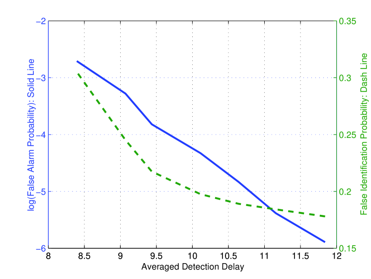
Figure 3: False alarm and false identification probability vs. averaged detection delay

Given that it is hard to efficiently compute the solution structure in (2), we compute the approximate optimal stopping rule in (28) and simulate its performance. We assign 5 nodes constructing a linear sensor array and assume that $f_{0}\sim\mathcal{N}(0,1)$ and $f_{1}\sim\mathcal{N}(1,1)$. The change point time is generated according to the geometric distribution with $\rho=0.01$, $\rho_{1}=0.1$ and $\rho_{2}=0.05$, respectively. According to (III), the false alarm probability with $\tau_{app}$ is

$$P[\tau_{app}\leq\Gamma]=\mathbb{E}\left\{{\sum\limits_{i=1}^{N}{{\pi_{N+1,\tau_{app}\left|i\right.}}}p_{\tau_{app}}^{i}}\right\}\leq\frac{c_{1}}{c_{1}+\rho}=\alpha.$$ (46)

Thus we have ${c_{1}}=\frac{\rho\alpha}{1-\alpha}$, where $\alpha$ is the maximum allowance for the false alarm probability, which could determine the required select $c_{1}$ value.

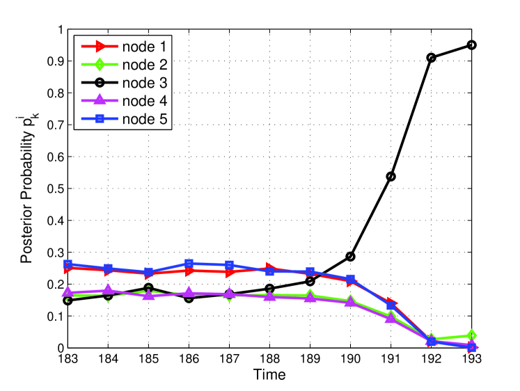
Figure 4: Posterior probability of which node that the change pattern first reaches

In Fig. 3, we illustrate the relationships among the false alarm probability, the false identification probability, and the averaged detection delay. We see that as the averaged detection delay increases, the false alarm probability decreases. When the averaged detection delay becomes large, the false identification probability does not decrease much and a probability floor appears, which is due to the fact that only the samples between the time when the change pattern reaches the first sensor and the time when it reaches the second sensor can be used to effectively distinguish the sensor that the change pattern first reaches. Since this part of the samples is limited, which will not increase with the detection delay, a false identification probability floor exists. In Fig. 4, we draw the posterior probability ${\bf{p}}_{k}^{i}$ over time, where we assume that the change pattern first reaches node 3, and then propagates to node 4. We see that as time goes, $p_{k}^{3}$ gradually becomes larger than the others, which indicates that node 3 should be identified. In Fig. 5, we show the relation between $\max\{p_{k}^{1},...,p_{k}^{N}\}$ and $\mathbb{E}\{\max\{p_{k+1}^{1},...,p_{k+1}^{N}\}|\mathcal{F}_{k}\}$ in (31). Since (31) is the key in deriving the our simplified rule, the fact that these two curves are close suggests that the performance of our low-complexity rule might be close to that of the optimal stopping rule in (2) and (III).

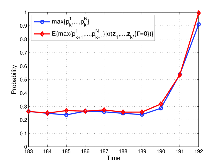
Figure 5: $\max\limits_{1\leq i\leq N}p_{k}^{i}$ vs. $\mathbb{E}\{\max\limits_{1\leq i\leq N}p_{k+1}^{i}|\mathcal{F}_{k}\}$

VI Conclusions

We have studied the quickest change point detection problem and the closest-node identification problem over a sensor array. We have proposed an optimal decision scheme combing the stopping rule and the identification rule to alarm the change happening and to determine the sensor closest to the change source. Since the structure the obtained optimal scheme is complex and impractical to implement, we have further proposed a scheme with a much simpler structure.

References

- [1] V. V. Veeravalli, “Decentralized quickest change detection,” IEEE Trans. Inform. Theory, vol. 47, no. 4, pp. 1657-1665, May 2001.
- [2] A. G. Tartakovsky and V. V. Veeravalli, “Asymptotically optimal quickest change detection in distributed sensor systems,” Sequential Analysis, vol. 27, no. 4, pp. 441-475, Nov. 2008.
- [3] O. Hadjiliadis, Hongzhong Zhang, and H. V. Poor, “One Shot Schemes for Decentralized Quickest Change Detection,” IEEE Trans. Inform. Theory, vol. 55, no. 7, pp. 3346-3359, Jul. 2009.
- [4] V. Raghavan and V. V. Veeravalli, “Quickest change detection of a Markov process across a sensor array,” IEEE Trans. Inform. Theory, vol. 56, pp. 1961-1981, Apr. 2010.
- [5] L. Lai, “Quickest Change Point Identification Across a Sensor Array,” IEEE Military Communications Conference (Milcom), Orlando, Oct. 2012. Submitted.
- [6] H. V. Poor and O. Hadjiliadis, Quickest Detection. Cambridge, UK: Cambridge University Press, 2008.
- [7] C. W. Baum and V. V. Veeravalli, “A sequential procedure for multihypothesis testing,” IEEE Trans. Inform. Theory, vol. 40, pp. 1994-2007, Nov. 1994.
- [8] S. Zacks, The theory of statistical inference. New York: John Wiley & Sons Inc., 1971.
- [9] A. G. Tartakovsky and G. Moustakides, “State-of-the-art in bayesian changepoint detection,” Seq. Anal., vol. 29, no. 2, pp. 125-145, Apr. 2010.