Search and Result Presentation in Scientific Workflow Repositories

Abstract

We study the problem of searching a repository of complex hierarchical workflows whose component modules, both composite and atomic, have been annotated with keywords. Since keyword search does not use the graph structure of a workflow, we develop a model of workflows using context-free bag grammars. We then give efficient polynomial-time algorithms that, given a workflow and a keyword query, determine whether some execution of the workflow matches the query. Based on these algorithms we develop a search and ranking solution that efficiently retrieves the top-$k$ grammars from a repository. Finally, we propose a novel result presentation method for grammars matching a keyword query, based on representative parse-trees. The effectiveness of our approach is validated through an extensive experimental evaluation.

1 Introduction

Data-intensive workflows are gaining popularity in the scientific community. Workflow repositories are emerging in support of sharing and reuse, either as part of a particular workflow system (e.g., VisTrails [4] or Taverna [28]) or independently within a particular community (e.g., myExperiment.org [29]). As workflows become more widely used, workflow repositories grow in size, making information discovery an interesting challenge.

Current workflow repositories, e.g., myExperiment.org, support tagging of workflows with keywords. Notably, because workflows are modular, users may wish to share and reuse components of a workflow [31]. It is thus important to support tagging, and to enable search, not just at the level of a workflow, but also at the level of modules and subworkflows.

Recent work considered search in workflow repositories [10, 25, 30], and also argued that, because workflows can be large and complex, it is important to provide usable result presentation mechanisms. In this paper we propose a novel search and result presentation approach for complex hierarchical workflows. We now illustrate our approach with an example.

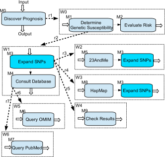
Figure 1: Disease succeptibility workflow.

$r_{1}:M_{0}\Rightarrow\{M_{1},M_{2}\}$   $r_{2}:M_{1}\Rightarrow\{M_{3},M4\}$

$r_{3}:M_{3}\Rightarrow\{M_{5},M_{3}\}$ $r_{4}:M_{3}\Rightarrow\{M_{8},M_{3}\}$ $r_{5}:M_{3}\Rightarrow\{M_{9}\}$

$r_{6}:M_{4}\Rightarrow\{\text{lookup},M_{6}\}$    $r_{7}:M_{4}\Rightarrow\{\text{lookup},M_{7}\}$

$r_{8}:M_{2}\Rightarrow\{\text{evaluate}\}$        $r_{9}:M_{5}\Rightarrow\{\text{23andMe}\}$

$r_{10}:M_{9}\Rightarrow\{\text{check}\}$          $r_{11}:M_{6}\Rightarrow\{\text{OMIM}\}$

$r_{12}:M_{7}\Rightarrow\{\text{PubMed}\}$      $r_{13}:M_{8}\Rightarrow\{\text{HapMap}\}$

Figure 2: Disease succeptibility workflow as a bag grammar.

Consider a workflow in Figure 1 that computes succeptibility of an individual to genetic disorders, and is based closely on [33]. This workflow takes a person’s genetic information in the form of single nucleotide polymorphisms (SNPs) as input, and produces an assessment of genetic disorder risk. The workflow is implemented by module $M_{0}$, which is composite, and, when invoked, executes modules $M_{1}$ and $M_{2}$ in sequence. Module $M_{1}$ expands the set of SNPs by considering known associations between SNP pairs and triplets. This module is composite, and has three alternative executions. In the first, the SNP set is expanded using a proprietary database of associations, e.g., 23andMe (module $M_{5}$), followed by a recursive call to $M_{3}$. In the second alternative, a public association database, e.g., HapMap (module $M_{8}$) is used, followed by a recursive call to $M_{3}$. The final alternative involves checking the retrieved results and terminating the recursion (module $M_{9}$). Having computed an expanded SNP set, the workflow goes on to look up any genetic disorders associated with the SNPs. This is implemented by module $M_{4}$, which has two alternative executions: it may issue a query to OMIM (module $M_{6}$) or to PubMed (module $M_{7}$). Having retrieved results from OMIM or from PubMed, the workflow terminates.

Suppose that this workflow exists in a repository, and that some of its modules are tagged. Let us assume the following assignment of keywords to workflow modules: $M_{2}$ (evaluate), $M_{4}$(lookup), $M_{5}$ (23andMe), $M_{6}$ (OMIM), $M_{7}$ (PubMed), $M_{8}$ (HapMap), and $M_{9}$ (check). It is not required that all modules be tagged, e.g., there is no keyword assigned to $M_{1}$ in our example. It is also possible, and even likely, that multiple keywords are assigned per module, and that keywords are reused across modules, and across workflows [31]. However, we do not use multiple or repeating keywords here, to simplify our example.

Suppose now that a user wants to know whether the workflow in Figure 1 matches a particular keyword query. Assuming “and” query semantics, answering this question amounts to determining if there exists some execution of the workflow in which all query keywords are present. For example, query $\{23andMe,HapMap\}$ matches an execution in which module $M_{3}$ is run twice, evaluating $M_{5}\rightarrow M_{3}$ (23andMe) on the first invocation, and $M_{8}\rightarrow M_{3}$ (HapMap) on the second invocation. Intuitively, this execution exists because of the combination of alternation and recursion at $M_{3}$.

On the other hand, there is no execution that matches $\{OMIM,PubMed\}$ because, once an alternative for expanding $M_{4}$ is chosen, then $M_{6}$ (OMIM) or $M_{7}$ (PubMed) is executed, and there is no recursion that allows $M_{4}$ to repeat, possibly choosing another branch.

It has recently been shown that complex hierarchical workflows can be naturally represented as context-free graph grammars involving recursion and alternation [1, 3]. We build on this work and adapt it to keyword search in workflows with tagged modules. Because of our proposed query semantics, observe that, while hierarchical workflow structure, alternation and recursion are important for determining whether a workflow matches a query, the graph structure within each composite module is unimportant for our purposes. This observation leads us to model scientific workflows as context-free bag grammars (also called commutative grammars [13]).

Figure 2 represents a bag grammar corresponding to the workflow in Figure 1. The bag grammar captures the hierarchical structure of the workflow (expansion of composite modules), alternation and recursion. Importantly, the grammar makes assignment of keywords to modules explicit, by including keywords as terminals. Note that keywords may annotate both atomic and composite modules, appearing in the corresponding grammar productions. So, $M_{4}$ is tagged with lookup, which is captured in productions $r_{6}$ and $r_{7}$.

Query $\{23andMe,HapMap\}$ matches the workflow in Figure 1, and we would now like to explain to the user how the match occurs. Let us now return to our example, and focus on result presentation. Providing a usable result presentation mechanism is important, because workflow specifications can be large, and each workflow can match a query in multiple ways, due in large part to recursion and alternation. We propose here a result presentation mechanism based on a novel notion of representative parse trees (rpTree for short). Figure 3 shows a particular rpTree for query $\{23andMe,HapMap\}$, with nodes representing bag grammar productions and terminals (see Figure 2), and edges corresponding to a firing of a production. Keyword matches occur at the leaves.

Intuitively, an rpTree represents a class of parse trees of a bag grammar that derive a particular set of terminals. An rpTree is an irredundant representative of its class, in the sense that it does not fire recursive productions that do not derive additional query-relevant terminals. For example, the rpTree in Figure 3 represents also a tree in which production $r_{3}$ is fired recursively twice, both times followed by $r_{9}$, and thus generating the terminal 23andMe twice. We will make the sense in which an rpTree is an irredundant representative of its class more precise in Section 5, and will show how rpTrees can be derived efficiently.

Figure 3: An rpTree for query $\{23andMe,HapMap\}$.

Contributions. The contributions of our paper include:

• A model of search and result presentation over keyword-annotated context-free bag grammars (Section 2): Although the motivation for our model is derived from the problem of searching workflow repositories, it is applicable to any other scenario involving search over context-free bag grammars, e.g., business processes, call structure of programs, or other hierarchical graph applications.

• Search and ranking algorithms (Sections 3 and 4): We give a bottom-up match algorithm, and develop an optimization, which borrows ideas from semi-naive datalog evaluation to avoid unproductive calculations. Next, translating probabilistic context-free grammars to our setting, we develop efficient search and ranking algorithms, and use them to identify top-$k$ grammars.

• Novel result presentation methods (Section 5): Since a workflow may match a query in many different ways, we develop a presentation mechanism to help the user understand how the keyword matches are most likely to occur. The mechanism is based on a novel notion of representative parse trees, which are the most probable parse trees that are structurally irredundant.

• Extensive experimental evaluations (Section 6): We use synthetic datasets to demonstrate the effectiveness of our approach. Our synthetic data is generated in a way that resembles characteristics of workflows in myExperiment.org, in terms of keyword assignment and workflow size. However, since current scientific workflow management systems do not yet allow that workflows be expressed as grammars, we are unable to use the myExperiment.org dataset directly in our experiments.

Related Work. Much effort [7, 17, 32] has been made recently to annotate scientific workflows to enable keyword search. As observed in [25], since scientific workflows are usually modeled as a three-dimensional graph structure when considering the expansions of composite modules (dashed edges in Figure 1), results on searching relational and XML data [5, 24, 35] or graph data [9, 18, 20, 34] can not be easily extended. [10, 25, 30] consider the scenario when alternation or recursion is not present in workflows. [23, 27] consider the scenario where nodes of XML documents exist with a probability (analogous to choice), however there is no recursion.

There are also extensive results in (context-sensitive) commutative grammars [14, 13], which have been cast as vector addition systems [21] and Petri nets [8]. Decidability issues of Petri nets are surveyed in [14], and are shown to be $\mathcal{NP}\mbox{-}complete$, directing focus towards more specific problems. We focus on a novel sub-problem,i.e., on whether there exists a bag that contains a keyword set and is accepted by a commutative grammar.

Most related to our work on matching and ranking is [12], which considers the more general problem of querying the structure of a specification using graph patterns. The paper gives a query evaluation algorithm of polynomial data complexity; the authors also consider the probability of the match in [11]. By considering each permutation of the keyword query $Q$ as a simple graph pattern, where each node represents a keyword and nodes form a chain connected by transitive edges, and taking the union of matching specifications for each permutation, these results could be used in our setting. However, our matching algorithm is optimized for queries that are sets of keywords, and is therefore simpler and considerably more efficient than [12] for this setting (see results in Section 6). Importantly, unlike [12], our solution does not require that the input grammar be transformed for each query. For this reason, our solution can be tailored to present results using representative parse trees (Section 5), while the solution of [12] cannot.

Also closely related to our match algorithm is [2], which gives a polynomial time algorithm for checking if the intersection of a context-free string grammar (which could represent the workflow specification) and a finite automaton (which could represent the query) results in an empty grammar; however, our match algorithm has a much better average case performance since it can terminate early if a match is found.

2 Model

In this section, we give background and definitions that will be used throughout the paper. We start with the definition of a context-free bag grammar, its language, and what it means for a search query with “and” semantics to match a grammar. We then introduce parse trees and derivation sequences. Finally, we define the notion of a repository of context-free bag grammars.

Definition 2.1.

(Context-free Bag Grammar)
A context-free bag grammar is a grammar $G=(\Sigma,\Delta,S,R)$ where $\Sigma$ is the set of symbols (variables and terminals), $\Delta\subset\Sigma$ is the set of terminals, $S$ is the start variable and $R$ is the set of production rules. For production $r\in R$, we denote by $head(r)\in\Sigma/\Delta$ the head of the production and $body(r)$ the bag of symbols in the body of the production. The language of the grammar, $L(G)$, is a set of bags whose elements are in $\Delta$: $L(G)=\;\{w\in\Delta^{*}|S\stackrel{{\scriptstyle*}}{{\Longrightarrow}}w\}$

We use context-free bag grammars to represent keyword-annotated scientific workflows, of the kind described in Figure 1, and with the corresponding grammar given in Figure 2. This grammar was derived by replacing each composite module (variable) with production rules that emit their keywords (as in rules $r_{6}$ and $r_{7}$ for module $M_{4}$), and adding a production rule for each atomic module (terminal) that emits its keyword (as in rules $r_{8}$ through $r_{13}$).

In the remainder of the paper, we will refer to a context-free bag grammar simply as a grammar, and will use $\\ productions(M)\subseteq R$ to denote the set of productions with $M$ in the head. For clarity, we also label productions.

Definition 2.2.

(Match) Given a grammar
$G=(\Sigma,\Delta,S,R)$ and a keyword query $Q\subseteq\Delta$, we say that $G$ matches $Q$ iff there exists some $X\in L(G)$ such that $Q\subseteq X$.

Example 2.1.

Consider the grammar $\\ G=(\{S,A,B,C,s_{1},s_{2},b,c\},\{s_{1},s_{2},b,c\},S,R)$, where $R$ is:

$$\begin{split}r_{1}:S&\Longrightarrow\{A,S\}\\ r_{2}:S&\Longrightarrow\{s_{1}\}\\ r_{3}:S&\Longrightarrow\{s_{2}\}\\ r_{4}:A&\Longrightarrow\{B,C\}\\ \end{split}$$

$$\begin{split}r_{5}:B&\Longrightarrow\{b\}\\ r_{6}:C&\Longrightarrow\{B\}\\ r_{7}:C&\Longrightarrow\{c\}\end{split}$$

The language of $G$ is $L(G)=\{(s_{1}+s_{2})(bc+bb)^{n}|n\in\mathbb{N}_{\geq 0}\}$. $G$ matches query $Q_{1}=\{s_{1},b\}$ since $Q_{1}\subseteq\{s_{1},b,b\}\in L(G)$. However, $G$ does not match $Q_{2}=\{s_{1},s_{2}\}$.

Since the language of a grammar can be infinite, we will need to focus our attention on a small sample of its elements in which a match can be found. For this, we will use the notion of parse trees and derivation sequences.

Definition 2.3.

(Parse Tree) A parse tree $T$ associated with a grammar $G=(\Sigma,\Delta,S,R)$ is a finite unordered tree where each interior node represents a production $r\in R$ and whose children represent $body(r)$, i.e. each child is either a terminal in $body(r)$ (in which case it is a leaf) or is a production whose head is a variable in $body(r)$. If $T$ consists of a single node, then it represents a terminal in $\Delta$. We use root(T), and leaves(T) to denote the root production and leaves of $T$, respectively.

For our purposes, a parse tree can be rooted at any terminal or production rather than just those whose head is $S$. Given a parse tree $T$ of a grammar, we denote by $paths(T)$ the bag of all root-to-leaf paths in $T$, $productions(T)$ the bag of productions applied in $T$, and $symbols(T)$ the set of symbols that appear in $productions(T)$.

We now define what portions of a keyword query a parse tree $T$ matches in terms of the query-relevant keywords generated by $T$, and adapt the notion of derivation sequence to our setting.

Definition 2.4.

(Generates) Given a grammar $G=(\Sigma,\Delta,S,R)$ and a query $Q\subseteq\Delta$, we say a parse tree $T$ generates the set of matching keywords $leaves(T)\cap Q$. A symbol $M\in\Sigma$ generates a set $X\subseteq Q$ iff one of its parse trees generates $X$.

Definition 2.5.

(Derivation Sequence) Given a grammar $G=(\Sigma,\Delta,S,R)$, we say a variable $A\in\Sigma/\Delta$ derives a symbol $B\in\Sigma$ iff there exists a parse tree $T$ where $root(T)\in productions(A)$, and $B\in symbols(T)$. Each path from $A$ to $B$ in $T$ is a sequence of productions called a derivation sequence. sequence $seq(A\mapsto B)$, we denote by $Set(seq(A\mapsto B))$ the bag of all productions applied in it.

If a variable $A$ derives a symbol $B$, we say $A$ is an ancestor of $B$ and $B$ is a descendant of $A$.

Definition 2.6.

(Simple Derivation Sequence) A derivation sequence is simple iff there is no production that appears in it more than once.

Intuitively, a simple derivation sequence is a derivation sequence where a recursion is fired at most once. It disregards unnecessary recursions and provides an upperbound for the complexity results in Section 3.1.

Definition 2.7.

(Distance) Given a grammar
$G=(\Sigma,\Delta,S,R)$, the distance from a variable $A\in\Sigma/\Delta$ to symbol $B\in\Sigma$ is the length of the longest simple derivation sequence for $A$ deriving $B$, denoted $d(A\mapsto B)$.The distance of a grammar is defined as the longest distance between any two symbols, denoted $d(G)$. It is easy to see $d(A\mapsto B)\leq d(G)\leq|R|$.

Example 2.2.

For the grammar in Example 2.1 there is only one simple derivation sequence for $S$ to derive $C$, i.e. $r_{1}r_{4}$. However, there are two simple derivation sequences to derive $B$, i.e. $r_{1}r_{4}$ and $r_{1}r_{4}r_{6}$. Hence $d(S\mapsto C)=2$ and $d(S\mapsto B)=3$. It is also easy to check that $d(G)=4$.

We end this section by discussing the notion of a repository of bag grammars. A repository of grammars is essentially a set of grammars in which symbols (modules) may be shared, but must be done so consistently. We assume that all grammars are proper, i.e. have no underivable symbols or unproductive variables.

Definition 2.8.

(Bag Grammar Repository) A bag grammar repository is a set of bag grammars such that for any two grammars $G_{1}=(\Sigma_{1},\Delta_{1},S_{1},R_{1})$ and $G_{2}=(\Sigma_{2},\Delta_{2},S_{2},R_{2})$, $\forall M\in(\Sigma_{1}\cap\Sigma_{2})$, $\bigcup\limits_{\begin{subarray}{c}r\in R_{1}\\ head(r)=M\end{subarray}}r=\bigcup\limits_{\begin{subarray}{c}r\in R_{2}\\ head(r)=M\end{subarray}}r$

3 Matching and Searching

In this section we give an efficient algorithm that, given a grammar $G$ and keyword query $Q$, determines whether $G$ matches $Q$. We start by presenting the basic algorithm, Match, which computes a fixpoint of subsets of matching keywords using a bottom-up approach over the hierarchy of nonterminals (Section 3.1). We then give an optimized match algorithm (Section 3.2), and extend the results to searching a repository of grammars.

Note that the matching problem is NP-complete with respect to combined (data and query) complexity, as shown in [12]. However, since query size is typically small (6 or fewer keywords), we focus on the data complexity and give a matching algorithm that is polynomial in the size of the grammar. As observed in the introduction, the algorithm in [12] could also be used here, since it considers a (more general) graph pattern query. However, our algorithm is optimized for keyword queries and is therefore simpler and considerably more efficient in our setting (see results in Section 6).

3.1 Keyword query match

We now give an algorithm, Match (Algorithm 1), which determines whether or not a grammar $G$ matches a keyword query $Q$. To do this, Match builds a parse tree bottom-up until some symbol generates $Q$, in which case $G$ matches $Q$, or until a fixpoint of query-relevant keywords is reached for each symbol, in which case $G$ does not match $Q$. It can be shown that the fixpoint will be reached at or before height $O(d(G))$, and that therefore the algorithm is polynomial in the size of the grammar (although exponential in the query size due to the cost of generating sets of query-relevant keyword sets).

Match generates for each symbol $M\in\Sigma$ the set $F(M)$ of sets of query-relevant keywords for $M$. It does so by considering parse trees of increasing height $i$, and calculating for each $M\in\Sigma$ the set $F_{i}(M)$ of sets of query-relevant keywords for $M$ that are derived by parse trees of height $\leq i$. For terminals $M\in\Sigma$ (which are the leaves in a parse tree), $F_{0}(M)$ can be calculated directly (line 2, ignore for now line 3). For variables $M\in\Sigma/\Delta$, $F_{0}(M)=\emptyset$ (line 4). It then calculates $F_{i}(M)$ by initializing it to $F_{i-1}(M)$ (line 7) or $\emptyset$, then considering each production $r$ with $M$ as head, taking the “product-union" of $F_{i-1}(\alpha_{j})$ for each $\alpha_{j}$ in $body(r)$, and adding the resulting set of query-relevant keywords to $F_{i}(M)$ (lines 9-11). This continues until the query is matched by some $M$ (line 12), or until a fixpoint is reached (for each symbol $M$, $F_{i}(M)=F_{i-1}(M)$, line 13).

Input: a grammar $G=(\Sigma,\Delta,S,R)$ and a query $Q\subseteq\Delta$

Output: boolean

/* $F(M):$ set of sets of query-relevant keywords for $M$ */

/* $F_{i}(M)=\{leaves(T)\cap Q|root(T)\in productions(M)$, $height(T)\leq i\}$ */

begin

      1 foreach $M\in\Delta$ do

            2 if $F(M)=\emptyset$ then $F_{0}(M)\leftarrow\{\{M\}\cap Q\}$

            

             /* for OptMatch (Algorithm 2) */

            3 else  $F_{0}(M)\leftarrow F(M)$

            

      4foreach $M\in\Sigma/\Delta$ do $F_{0}(M)\leftarrow\emptyset$

      

      5 $i\leftarrow 0$ // a counter for iteration times

      6 L: $i\leftarrow i+1$

      7 foreach $M\in\Delta$ do $F_{i}(M)\leftarrow F_{i-1}(M)$

      

      8 foreach $M\in\Sigma/\Delta$ do $F_{i}(M)\leftarrow\emptyset$

      

      9 foreach production $r:M\rightarrow\alpha_{1}\alpha_{2}\ldots\alpha_{n}\in R$ do

             /* Construct parse trees rooted at $r$ */

            10 foreach $X_{1}\in F_{i-1}(\alpha_{1})$, $\ldots X_{n}\in F_{i-1}(\alpha_{n})$ do

                  11 $F_{i}(M).addElement(\bigcup\limits_{j=1}^{n}{X_{j}})$

            

      12if $\exists M\in\Sigma,Q\in F_{i}(M)$ then  return true

      

      13 if $\exists M\in\Sigma/\Delta,~{}F_{i}(M)\not=F_{i-1}(M)$ then goto $L$

      

      14 return false

Algorithm 1 Match

Example 3.1.

Consider the grammar in Example 2.1 and query $Q=\{b,c\}$. Initially, $F_{0}(s_{1})=F_{0}(s_{2})=\{\emptyset\}$, $F_{0}(b)=\{\{b\}\}$, $F_{0}(c)=\{\{c\}\}$, and $F_{0}(S)=F_{0}(A)=F_{0}(B)=F_{0}(C)=\emptyset$ (lines 1-4). In the first iteration of L ($i=1$), we add to $F_{1}(S)$ the set $\emptyset$ (after processing rule $r_{1},r_{2},r_{3}$). After processing all other productions, we have $F_{1}(A)=\emptyset$, $F_{1}(B)=\{\{b\}\}$, and $F_{1}(C)=\{\{c\}\}$. We then proceed to the second iteration ($i=2$). During this iteration, when rule $r_{4}$ is processed, we add to $F_{2}(A)$ (which was initialized to $F_{2}(A)=\emptyset$) the product of $F_{1}(B)$ and $F_{1}(C)$, at each step taking the union of the two elements (e.g. $\{b\}\cup\{c\}=\;\{b,c\}$), resulting in $F_{2}(A)=\{\{b,c\}\}$. Since $Q\in F_{2}(A)$, Match terminates. If this early termination condition were omitted, the fixpoint would have been reached in the fifth iteration, since $F_{5}(S)=F_{4}(S)$, $F_{5}(A)=F_{4}(A)$, $F_{5}(B)=F_{4}(B)$, $F_{5}(C)=F_{4}(C)$.

We now show that the data complexity of Match is $O(|G|*d(G))$. We start by showing that it will reach a fixpoint in $d(G)*(|Q|+1)+|Q|$ iterations by proving that if a symbol $M\in\Sigma$ generates a set $X\subseteq Q$, then there exists a parse tree $T$ rooted at $r\in productions(M)$ of height at most $d(G)*(|Q|+1)+|Q|$ such that $leaves(T)\cap Q=X$.

Lemma 3.1.

Given a grammar $G=(\Sigma,\Delta,S,R)$ and a query $Q\subseteq\Delta$, $\forall M\in\Sigma,~{}\forall X\subseteq Q$, $height(M,X)\leq d(G)*(|Q|+1)+|Q|$.

Proof.

Note that if $M\in\Sigma$ generates $X\subseteq Q$, then the parse trees that generate $X$ fall in one of two classes: (1) each child subtree generates a subset of $X$, in which case we say the parse tree produces the set $X$; (2) some child subtree generates $X$ by itself, in which case we say the parse tree broadcasts $X$.

We denote by $height(M,X)$ ($M\in\Sigma/\Delta,X\subseteq Q$) the minimum height of parse trees of $M$ that generate $X$;
$height(M,X)=-1$ if $M$ cannot generate $X$. Similarly, we denote by $height_{p}(M,X)$ ($height_{b}(M,X)$) the minimum height of parse trees of $M$ that produce (broadcast) $X$. For $height_{p}(M,X)$ we have the following:

$$\small height_{p}(M,X)=\begin{cases}0&\text{if }M\in\Delta,X=\{M\}\cap Q\\ -1&\text{if }M\in\Delta,X\not=\{M\}\cap Q\\ -1&\text{if }M\in\Sigma/\Delta,|X|\leq 1\end{cases}$$ (1)

$$\small height_{p}(M,X)\leq 1+\max\limits_{M^{\prime}\in\Sigma,X^{\prime}\subset X}height(M^{\prime},X^{\prime})$$ (2)

Turning to $height_{b}(M,X)$, we have:

$$\small height_{b}(M,X)\leq d(G)+\max\limits_{M^{\prime}\in\Sigma}{height_{p}(M^{\prime},X)}$$ (3)

$$\small height(M,X)\leq\max(height_{p}(M,X),height_{p}(M,X))$$ (4)

So we have $height(M,X)\leq d(G)*(|Q|+1)+|Q|$. ∎

Using Lemma 3.1 we can prove the following.

Theorem 1.

The data complexity of Match is
$O(|G|*d(G))$.

Proof.

The size of a grammar $G=(\Sigma,\Delta,S,R)$ is defined as the sum of the sizes of its productions,
$|G|=\sum\limits_{r\in R}{(1+|body(r)|)}$. By Lemma 3.1 we know that the number of iterations of Algorithm 1 is bounded by $d(G)*(|Q|+1)+|Q|$. Each iteration (loop L) of Algorithm 1 processes all productions, each of which takes $O(|body(r)|*2^{|Q|})$. Since the query size is considered as a constant, this yields a total time of $O(|G|*d(G))$. ∎

3.2 Optimized keyword query match

We now introduce two improvements to Match, one of which avoids unproductive calculations introduced by variables that are fixed early, and the other of which reduces the size of $F_{i}(M)$.

Optimization 1: Symbol Dependencies Borrowing ideas from semi-naive Datalog evaluation, we observe that a grammar yields symbol dependencies through the head and body structure of rules, e.g. that in Match the start variable $S$ will not be fixed until $A$ is fixed (a variable $M$ is fixed in the $i^{th}$ iteration, iff $\forall j>i,F_{j}(M)=F_{i}(M)$, $\forall j<i,F_{j}(M)\subset F_{i}(M)$). The first optimization is to avoid unproductive calculations introduced by variables which are fixed early.

Given a grammar $G=(\Sigma,\Delta,S,R)$, we create a precedence graph $\cal{G=(V,E)}$ of symbols as follows: $\cal{V}$= $\Sigma$, and a directed edge $(M,M^{\prime})$ is added to $\cal{E}$ iff $\exists r\in R,head(r)=M,body(r)\ni M^{\prime}$. $\cal G$ has a directed cycle iff $G$ is recursive. Two symbols are mutually recursive iff they participate in the same cycle of $\cal G$. Mutual recursion is an equivalence relation on $\Sigma$, where each equivalence class corresponds to a strongly connected component of $\cal G$. Denote by $[M]$ the symbol equivalence class of $M$, and perform a topological sort of $\cal G$ to construct a list $[M_{1}],\,[M_{2}]\ldots[M_{n}]$. Clearly, if there is a path from $[M_{j}]$ to $[M_{i}]\,(i<j)$, then symbols in $[M_{i}]$ are fixed earlier than symbols in $[M_{j}]$; symbols in the same equivalence class are fixed in the same iteration.

Optimization 2: Set Domination We note that an element in $F_{i}(M)$ is useless if it is a subset of (dominated by) another element in $F_{i}(M)$. For example, $\{b\}$ is useless in $F_{3}(A)=\{\{b\},\{b,c\}\}$ of Example 3.1. Using set domination, $|F(M)|$ decreases from $2^{|Q|}$ to $\binom{|Q|}{\lfloor|Q|/2\rfloor}$.

Input: a grammar $G=(\Sigma,\Delta,S,R)$ and a query $Q\subset\Delta$

Output: boolean

Initialization

Precompute the symbol equivalence classes $[M]$

Precompute the topological order of the symbol equivalence classes, $T\_order$

begin

      1 foreach $M\in\Sigma$ do $F(M)=\emptyset$

      

      2 foreach $[M]\in T\_order$ do

             // Find the relevant productions of $[M]$

            3 $R^{\prime}\leftarrow\{r|r\in R,head(r)\in[M]\}$

            4 $\Sigma^{\prime}\leftarrow\bigcup\limits_{r\in R^{\prime}}(head(r)\cup body(r))$

             /* all descendants have been fixed and hence are treated as terminals */

            5 $\Delta^{\prime}\leftarrow\Sigma^{\prime}/\ ([M]/\Delta)$

             /* $F(\cdot)$ is a global variable visible for both $OptMatch()$ and $Match()$ */

            6 if $Match(Q,\Sigma^{\prime},\Delta^{\prime},M,R^{\prime})$ then return true

            

            

      7return false

Algorithm 2 OptMatch

Algorithm 2 gives the optimized algorithm, OptMatch. Note that the topological order of symbol equivalence classes is query-independent and can be precomputed. Line 6 of OptMatch calls Match for the current equivalence class. $F(M)$ is global, and is used in lines 2-3 of Match. Set domination is captured in the addElement method in Match.

Example 3.2.

Consider the grammar in Example 2.1 and query $Q=\{b,c\}$. One topological order of the symbol equivalence classes is $[b],[c],[B],[C],[s_{1}],[s_{2}],[A],[S]$ where each of the classes consists of the symbol itself. For $[b]$, $R^{\prime}=\emptyset,~{}\Sigma^{\prime}=\{b\},~{}\Delta^{\prime}=\{b\}$ (lines 3-5); after calling Match (line 6), $F(b)=\{\{b\}\}$. Similarly, $F(c)=\{\{c\}\}$, $F(B)=\{\{b\}\}$. Now we process $[C]$ where $R^{\prime}=\{r_{6},r_{7}\},~{}\Sigma^{\prime}=\{C,B,c\},~{}\Delta^{\prime}=\{B,c\}$. When calling Match for $[C]$, the initialization results in $F_{0}(B)=F(B)=\{\{b\}\},~{}F_{0}(c)=F(c)=\{\{c\}\}$ (line 3 of Algorithm 1). At the end of Match, we get $F(C)=\{\{b\},\{c\}\}$. We can check that OptMatch terminates after processing $[A]$ since $Q\in F(A)=\{\{b,c\}\}$.

3.3 Searching a bag grammar repository

Given a bag grammar repository and query $Q$, we must retrieve all grammars that match $Q$. A straightforward way to do this is to run $OptMatch$ over each grammar. This way a grammar that is reused by other grammars will be processed multiple times. One solution is to union productions of all grammars to form a universal grammar. However, this grammar would be too large to fit in memory.

We therefore process grammars one by one while recognizing grammar reuse; an individual grammar can be assumed to fit in main memory. We first build inverted indexes to help identify candidate grammars, i.e. grammars in which every keyword of the query appears (although they may not simultaneously occur in some bag in the language of the grammar). Each index maps a keyword to a list of grammars in which the keyword appears. Given a query, we find candidate grammars by intersecting the corresponding lists.

We then process candidate grammars (using $OptMatch$) so that a grammar is always processed earlier than the grammars that reuse it. Specifically, we create a precedence graph where nodes of the graph are grammars, and there is an edge from $G_{i}$ to $G_{j}$ iff $G_{j}$ reuses $G_{i}$ (i.e. the start module of $G_{i}$ appears in $G_{j}$ as a variable). The graph is a $DAG$, since there is a temporal dimension to reuse. A topological order of the $DAG$ is the order in which grammars are processed.

We cache intermediate results ($F(S)$) for grammars that are reused and clean them from memory when there are no unprocessed grammars that reuse them. In this way, we balance memory size and overhead of redundant computations.

4 Ranking

For large repositories of grammars, more grammars may match a query than can be shown to a user, motivating ranking. In this section we describe a relevance measure based on probabilistic grammars (Section 4.1) and develop an algorithm for computing the relevance of a grammar to a query (Section 4.2). We also describe an efficient top-$k$ algorithm (Section 4.3).

4.1 Semantics of relevance

Probabilistic context-free grammars (PCFG) have been used in applications such as natural language processing (NLP) to analyze the probability that a string is generated by a particular grammar. It is therefore natural to use them for ranking. Although our grammars generate bags rather than strings, the formalism applies literally in our setting.

Definition 4.1.

(Probabilistic Context-Free Bag
Grammar) A probabilistic context-free bag grammar $G=(\Sigma,\Delta,S,R,\rho)$ is a context-free bag grammar in which each production is augmented with a probability $\rho:R\rightarrow(0,1]$ such that $\forall M\in\Sigma/\Delta,~{}\sum\limits_{r\in productions(M)}\rho(r)=1$.

In a PCFG, which production $r\in productions(M)$ is chosen at a given composite module $M$ is independent of the choices that lead to $M$. Thus, the probability of a parse tree $T$, which we will denote $\rho(T)$, is the product of the probabilities of productions used in the derivation, i.e., $\rho(T)=\prod\limits_{r\in productions(T)}{\rho(r)}$.

Probabilities of productions in $G$ may be given by an expert or mined from the corpus. In this paper, we do not consider how these probabilities are derived, but note that much work on the topic has been done in the NLP community [26], and the techniques are likely applicable here.

Given a grammar $G$ and a query $Q$, our goal is to compute a relevance score, denoted $score(G,Q)\in[0,1]$, representing the likelihood of $G$ to generate a parse tree that matches $Q$. We want these scores to be comparable across grammars, which would enable us to say that, if $score(G,Q)>score(G^{\prime},Q)$, then $G$ is more query-relevant than $G^{\prime}$. Generating scores that are comparable across grammars turns out to be tricky, because, as we show next, parse trees of probabilistic context-free bag grammars may not form a valid probabilistic space.

Consider the grammar $G^{\prime}$ in Figure 4 that consists of two productions, chosen with equal probability (probabilities are indicated in parentheses). Since $G^{\prime}$ is recursive, it generates an infinite number of parse trees that match query $Q=\{a\}$. Two of these are shown in Figure 4.

$$r_{1}:S\Longrightarrow \{S,S,S\} (0.5)$$

$$r_{2}:S\Longrightarrow \{a\} (0.5)$$

Figure 4: Recursive bag grammar

These trees have probabilities: $\rho(T_{1})=0.5$ and $\rho(T_{2})=0.5^{4}=0.0625$. Unfortunately, it is not possible to compute a normalization factor by summing the probabilities of the infinitely many parse trees, because this sum is irrational [6]. Generally, given a PCG $G=(\Sigma,\Delta,S,R,\rho)$, and a query $Q\subseteq\Delta$, it is customary to define a relevance score $score(G,Q)$ using max or sum semantics.

$$\small score_{sum}(G,Q)=\sum\limits_{\begin{subarray}{c}r(T)\in R(S)\\ Q\subseteq leaves(T)\end{subarray}}{\rho(T)}/\sum\limits_{r(T)\in R(S)}{\rho(T)}$$ (5)

$$\small score_{max}(G,Q)=\max\limits_{\begin{subarray}{c}r(T)\in R(S)\\ Q\subseteq leaves(T)\end{subarray}}{\rho(T)}/\max\limits_{r(T)\in R(S)}{\rho(T)}$$ (6)

Sum semantics is intuitive: we normalize the total probability of all parse trees matching the query by the total probability of all parse trees. Unfortunately, as we argued above, this value cannot be computed because probabilities may be irrational. It was shown in [15] that $score_{sum}$ may be approximated by solving a monotone system of polynomial equations. However, this approach is in PSPACE, and is very expensive in practice.

Motivated by these considerations, we opt for max scoring semantics, where the score of a grammar for a query is computed by dividing the probability of the most likely parse tree matching the query by the probability of the over-all most likely parse tree. This semantics is reasonable, and, as we will show next, $score_{max}(G,Q)$ can be computed efficiently. We refer to $score_{max}(G,Q)$ simply as $score(G,Q)$ in the remainder of the paper.

4.2 Computing the score of a workflow

We now present Algorithm 3, Score, which computes the relevance score of grammar $G$ for query $Q$ per Equation 6. This is a fixpoint algorithm that is similar in spirit to Match.

Note that the algorithm of [11] can also be used to compute the relevance score of grammar $G$ for query $Q$. This algorithm uses a similar framework as [12], and so is very general, but is less efficient in our particular scenario. We will give experimental support to this claim in Section 6.3.

Recall from Match that $F_{i}(M)$ represents the set of sets of query-relevant keywords that module $M$ matches, and that are derived by parse trees of height $\leq i$. Score uses $F_{i}(M)$ and a data structure $\rho_{i}(M,X)$, in which it stores, for each $X\in F_{i}(M)$, the score of the corresponding parse tree. Like Match, Score manipulates a global data structure $F(M)$; Score also maintains the corresponding global $\rho(M,X)$. These data structures will become important when we consider an optimization, called OptScore.

Input: grammar $G=(\Sigma,\Delta,S,R)$ and query $Q\subseteq\Delta$

Output: double

begin

      1 foreach $M\in\Delta$ do

            2 if $F(M)=\emptyset$ then

                  $F_{0}(M)\leftarrow\{\{M\}\cap Q\}$; $\rho_{0}(M,\{M\}\cap Q)\leftarrow 1.0$

            3else

                   $F_{0}(M)\leftarrow F(M)$ $\forall X\in F_{0}(M),\rho_{0}(M,X)\leftarrow\rho(M,X)$

            

      

      4foreach $M\in\Sigma/\Delta$ do $F_{0}(M)\leftarrow\emptyset$

      

      

      5$i\leftarrow 0$ // a counter for iteration times

      6 L: $i\leftarrow i+1$

      7 foreach $M\in\Delta$ do

            $F_{i}(M)\leftarrow F_{i-1}(M)$

             $\forall X\in F_{i}(M),\rho_{i}(M,X)\leftarrow\rho_{i-1}(M,X)$

      8foreach $M\in\Sigma/\Delta$ do $F_{i}(M)\leftarrow\emptyset$

      

      9 foreach production $r:M\rightarrow\alpha_{1}\alpha_{2}\ldots\alpha_{n}\in R$ do

            10 foreach $X_{1}\in F_{i-1}(\alpha_{1})$, $\ldots X_{n}\in F_{i-1}(\alpha_{n})$ do

                   $X\leftarrow\bigcup\limits_{j=1}^{n}{X_{j}}$ $prob\leftarrow\rho(r)\times\prod_{j=1}^{n}{\rho_{i-1}(\alpha_{j},X_{j})}$

                   if $X\not\in F_{i}(M)$ then  $\rho_{i}(M,X)\leftarrow prob$

                  

                   else $\rho_{i}(M,X)\leftarrow\max(\rho_{i}(M,X),prob)$

                  11 $F_{i}(M).addElement(X)$

            

      13 if $\exists M\in\Sigma/\Delta,~{}F_{i}(M)\not=F_{i-1}(M)$ then goto $L$

      

       if $Q\not\in F(S)$ then return $0.0$

       // not matching

       if $\exists M\in\Sigma,\exists X\in F_{i}(M),~{}\rho_{i}(M,X)>\rho_{i-1}(M,X)$ then goto $L$

      

       $F(M)=F_{i}(M);~{}\rho(M,X)=\rho_{i}(M,X)$

       return $\rho(S,Q)/\rho_{max}(S)$

Algorithm 3 $Score$

Algorithm Score starts by storing the set of query-relevant keywords annotating each terminal module $M$ in $F_{0}(M)$, and by recording the probability score of 1.0 in $\rho_{0}$. Next, for non-terminal modules, $F_{0}(M)$ is initialized to an empty set. The bulk of the processing happens next, where, at each iteration $i$, we consider each production $r$ rooted at $M$, and generate all sets of query terminals resulting from parse trees of height at most $i$ rooted at $M$. We record the resulting subset of query keywords $X$ if this subset has not been seen before, or it if is the highest-scoring parse tree for this subset at the current round. We compute the probability score of a parse tree resulting from production $r$ as the product of the probabilities of its subtrees and the probability of $r$.

Score terminates when either no new subsets of the query are generated, or no better (more probable) derivations of existing subsets are found. Score returns the normalized probability of the most probable derivation tree matching $Q$. Note that normalization factor $\rho_{max}(S)$ is query-independent and can be computed by invoking $Score(G,\emptyset)$. We compute $\rho_{max}(S)$ offline and store it for future use.

Example 4.1.

Consider the grammar in Example 2.1 and assume that productions with the same head are equally likely. Given the query $Q=\{b,c\}$, Score calculates $\rho_{max}(S)=1/3$, $\rho(S,Q)=\frac{1}{3}*\frac{1}{3}*\frac{1}{2}$ and returns $\frac{1}{3}*\frac{1}{3}*\frac{1}{2}/\rho_{max}(S)=\frac{1}{6}$ when it terminates at the end of the $5^{th}$ iteration.

The worst-case running time of Score is polynomial in the size of the grammar. This can be shown by a similar argument as for Match (Section 3.1), and is based on the observation that, for any symbol $M$, the height of the most probable parse tree generating any subset of $Q$ is bounded by $\leq d(G)*(|Q|+1)+|Q|$.

We also developed an optimized version of Score, which we call OptScore. We do not detail the OptScore algorithm here, but note that it is based on the two optimizations performed in OptMatch. The first optimization, symbol dependencies, identifies equivalence classes of modules of $G$ based on their reuse of variables on the right-hand-side of productions. OptScore computes a topological ordering among equivalence classes, and runs algorithm Score for each class in reverse topological order, saving intermediate results in global data structures $F(M)$ and $\rho(M,X)$. The second optimization, set domination, includes probabilities in the notion of domination: a set $X_{1}\in F_{i}(M)$ dominates $X_{2}\in F_{i}(M)$ iff $X_{1}\supset X_{2}$ and $\rho_{i}(M,X_{1})\geq\rho_{i}(M,X_{2})$.

$$\begin{split}r_{1}:S\Longrightarrow&\{S,A\}\\ r_{2}:S\Longrightarrow&\{S,S,B\}\\ r_{3}:S\Longrightarrow&\{s\}\\ r_{4}:A\Longrightarrow&\{a\}\\ r_{5}:B\Longrightarrow&\{B,S\}\\ r_{6}:B\Longrightarrow&\{b\}\\ \end{split}$$

Figure 5: An example of a grammar.

4.3 Identifying the top-$k$ workflows

We conclude our discussion of ranking by presenting an efficient way to retrieve, and compute the scores of, the top-$k$ workflows in a repository. Given a repository, a query $Q$, and an integer $k$, a naive approach is to compute $score(G,Q)$ using, e.g., OptScore, sort grammars in decreasing order of score, and return the top-$k$. Here, $OptScore$ may be executed on the entire repository, or only on its promising subset, leveraging an inverted index that maps each keyword to the set of workflows in which it appears. Even assuming that only the grammars matching $Q$ are considered (i.e., grammars for which Match(G,Q) returns true), this naive approach will still require us to compute $score(G,Q)$ for many more than $k$ grammars.

We use the Threshold Algorithm (TA) [16] to limit the number of score computations. Our use of TA is based on the observation that $score(G,Q)\leq\min_{X\subset Q}score(G,X)$. In particular, $score(G,Q)$ is at most as high as the score of $G$ for any single-keyword subset of $Q$.

We leverage this observation and build inverted lists, one per keyword $a$, storing all grammars $G$ that match $a$, in decreasing order of $score(G,\{a\})$. Then, given a multi-keyword query $Q$, we access the query-relevant lists sequentially in parallel, and compute $score(G,Q)$ for the first $k$ grammars. We refer to the current $k^{th}$ highest score as $\theta$, and we update $\theta$ as the algorithm proceeds.

We consider grammars in inverted list order, and, when an unseen grammar $G$ is encountered, retrieve its entries from all inverted lists with random accesses, and compute the score upper-bound $ub(G,Q)=\min_{a\in Q}score(G,\{a\})$. If $ub(G,Q)>\theta$, we compute $score(G,Q)$ using an algorithm from Section 4.2 and update $\theta$ if necessary. TA terminates when the score upper-bound of unseen grammars, computed as the minimum of current scores in the relevant inverted lists, is lower than $\theta$.

5 Result Presentation

Since grammars may be large and complex objects, it is important to develop presentation mechanisms that help the user understand where keyword matches occur in the result grammars. Interestingly, a single grammar may match a query in many ways, more than can be shown to a user. In Section 4 we proposed to compute probabilities of parse trees, and to use these probabilities to rank grammars. In this section, we build on this idea and propose to choose the most probable parse trees that are structurally irredundant. We refer to such trees as representative parse trees, and describe them in Section 5.1. We then give an algorithm for finding the top-$k$ representative parse trees for a given grammar in Section 5.2.

5.1 Representative parse trees

Recursion gives rise to structural redundancy. Consider the grammar in Figure 5, and its parse trees $T_{1}$ and $T_{2}$. These trees both match query $Q=\{s,a\}$. Both trees fire the same productions in the same order, and, while $T_{1}$ cuts through the chase, $T_{2}$ loops by firing $r_{1}$ twice in sequence, and by generating $a$ along the path $S\rightarrow A\rightarrow a$ twice. The concept of a representative parse tree (rpTree for short), which we define next, models the intuition that, while both trees match the query in the same way (by firing the same productions in the same order), $T_{1}$ is more concise than $T_{2}$.

For convenience, we will sometimes represent parse trees as bags of paths, denoted $paths(T)$. Recall that a path is a sequence of productions that ends with a terminal, e.g., $r_{1}r_{3}s$ is a path in $T_{1}$ in Figure 5. We can represent $T_{1}$ as $paths(T_{1})=\{r_{1}r_{3}s,~{}r_{1}r_{4}a\}$. Note that the paths representation may be ambiguous i.e. the same bag of paths may correspond to two different parse trees (See Figure 6).

$$\begin{split}r_{1}:S\rightarrow&SS\\ r_{2}:S\rightarrow&AB\\ r_{3}:A\rightarrow&a_{1}\\ r_{4}:A\rightarrow&a_{2}\\ r_{5}:B\rightarrow&a_{1}\\ r_{6}:B\rightarrow&a_{3}\\ \end{split}$$

Figure 6: $paths(T_{1})=paths(T_{2})$ while $T_{1}\not=T_{2}$

Definition 5.1.

(Path Subsumption) Path $p$ subsumes path $p^{\prime}$, denoted $p\prec p^{\prime}$ if $p$ is a sub-sequence of $p^{\prime}$.

For example, $r_{1}r_{3}s\prec r_{1}r_{1}r_{3}s$. Note that, since a path ends with a terminal, if $p\prec p^{\prime}$ then the paths must end in the same terminal. We use path subsumption to define the main concept of this section, parse tree subsumption.

Definition 5.2.

(Parse Tree Subsumption) Parse tree $T$ subsumes parse tree $T^{\prime}$, denoted $T\prec T^{\prime}$, iff $head(root(T))=head(root(T^{\prime}))$ and there exists an onto mapping from $paths(T^{\prime})$ to $paths(T)$, in which, if $p^{\prime}\in paths(T^{\prime})$ is mapped to $p\in paths(T)$ then $p\prec p^{\prime}$.

For example, consider the parse trees in Figure 5. Observe that $T_{1}\prec T_{2}$ according to Definition 5.2. The onto mapping from $paths(T_{2})$ to $paths(T_{1})$ is: $r_{1}r_{1}r_{3}s\rightarrow r_{1}r_{3}s$, $r_{1}r_{1}r_{4}a\rightarrow r_{1}r_{4}a$ and $r_{1}r_{4}a\rightarrow r_{1}r_{4}a$. In contrast, no subsumption holds between parse trees $T_{2}$ and $T_{3}$.

Definition 5.3.

(Representative Parse Tree) A representative parse tree (rpTree) $T$ of a grammar $G$ is a parse tree s.t. there does not exist a parse tree $T^{\prime}$ of $G$ that subsumes $T$.

We now list several important properties of rpTrees. Given a path $p$, we denote by $len(p)$ the length of $p$.

Theorem 2.

A grammar $G$ matches a query $Q$ iff there exists an rpTree $T$ in $G$ that generates $Q$.

Proof.

The forward direction is trivial. For the reverse, recall that if a grammar $G$ matches $Q$, then $Q$ must be contained in the leaves of some parse tree for $G$. Then it must also be contained in the leaves of an rpTree, since an rpTree generates the same terminal set as the trees that it subsumes. ∎

Lemma 5.1.

If a parse tree is representative, then all its subtrees are also representative.

Proof.

Proof is by contradiction. Let $T$ be an rpTree. Suppose a subtree of $T$ denoted by $T_{sub}$ is subsumed by tree $T^{\prime}_{sub}$. Let $T^{\prime}$ be the tree obtained from $T$ by replacing $T_{sub}$ with $T^{\prime}_{sub}$. It is easy to see that $T^{\prime}\prec T$, which contradicts that $T$ is an rpTree tree. ∎

The converse is not true, see $T_{2}$ in Figure 5 for a counter-example. One can verify that the two child subtrees of $T_{2}$ are rpTrees. $T_{2}$ however is subsumed by $T_{1}$ and hence is not representative.

Lemma 5.2.

Given parse trees $T$ and $T^{\prime}$, if $T\prec T^{\prime}$ then $height(T)\leq height(T^{\prime})$.

Proof.

Let $p_{max}$ be one of the longest paths in $paths(T)$. Then $height(T)=len(p_{max})$. Since $T\prec T^{\prime}$, for any path $p\in paths(T)$, there is a path $p^{\prime}\in paths(T^{\prime})$ s.t. $p\prec p^{\prime}$. Let $p^{\prime}$ be a path in $paths(T^{\prime})$ that $p_{max}$ subsumes. Note that $len(p)\leq len(p^{\prime})$ if $p\prec p^{\prime}$. Then $height(T)=len(p_{max})\leq len(p^{\prime})\leq height(T^{\prime})$. ∎

Consider trees $T_{3}$ and $T_{4}$ in Figure 5. These trees are of the same height, yet $T_{3}\prec T_{4}$.

Lemma 5.3.

If $T\prec T^{\prime}$ and $height(T)=height(T^{\prime})$, then $T$ and $T^{\prime}$ must be rooted at the same production.

Proof.

Let $p_{max}$ be one of the longest paths in $T$. Since $T\prec T^{\prime}$, there exists a path $p^{\prime}\in paths(T^{\prime})$ s.t. $p_{max}\prec p^{\prime}$. Thus $height(T)=len(p_{max})\leq len(p^{\prime})\leq height(T^{\prime})$. Since $height(T)=height(T^{\prime})$, $len(p_{max})=len(p^{\prime})$. Recall that $p_{max}\prec p^{\prime}$. Thus $p_{max}=p^{\prime}$. Since $p_{max}~{}(p^{\prime})$ starts with the root production of $T~{}(T^{\prime})$, $T$ and $T^{\prime}$ are rooted at the same production. ∎

Theorem 3.

Given trees $T$ and $T^{\prime}$, the time complexity of checking if $T\prec T^{\prime}$ is polynomial in tree size.

Proof.

We prove the theorem by giving a polynomial algorithm of checking if $T\prec T^{\prime}$.

The algorithm starts by computing a mapping $f:paths(T^{\prime})\rightarrow paths(T)^{*}$ such that for any path $p^{\prime}\in paths(T^{\prime})$, $f(p^{\prime})\ni p$ iff $p\prec p^{\prime}$. Note that if $\exists p^{\prime}\in paths(T^{\prime}),f(p^{\prime})=\emptyset$ then $T\not\prec T^{\prime}$.

We then build a flow network s.t. the network has maximum flow $|paths(T)|$ iff there exists a surjective mapping $g:paths(T^{\prime})\rightarrow paths(T)$ s.t. if $g(p^{\prime})=p$, $p\prec p^{\prime}$. The flow network is built as follows. Let $N=(V,E)$ be a network with $s,t$ being the source and the sink of $N$, respectively. For each path $p\in paths(T)$ $(p^{\prime}\in paths(T^{\prime}))$, there is a node $p$ $(p^{\prime})\in V$. For each $p\in paths(T)$, there is an edge from $p$ to sink $t$ in $E$. For each $p^{\prime}\in paths(T^{\prime})$, there is an edge from source $s$ to $p^{\prime}$ in $E$ and an edge from $p^{\prime}$ to $p$ for any $p\in f(p^{\prime})$. Every edge has a capacity of $1$. It is easy to see that $N$ has maximum flow $|paths(T)|$ iff such $g$ exists.

It is easy to see that $T\prec T^{\prime}$ iff $\forall p^{\prime}\in paths(T^{\prime}),f(p^{\prime})\not=\emptyset$ and $g$ exists.

Note that given two paths $p,p^{\prime}$, checking if $p\prec p^{\prime}$ can be done in time $len(p)+len(p^{\prime})$, i.e. $O(height(T^{\prime}))$. It takes $O(|paths(T)|*|paths(T^{\prime})|*height(T^{\prime}))$ to compute $f$. In the worst case, the size of $f$ could be $|paths(T)|*|paths(T^{\prime})|$. It takes $O(|paths(T)|*|paths(T^{\prime})|)$ to build the flow network. Using the Ford-Fulkerson algorithm [22], it takes $O(|paths(T)|^{2}*|paths(T^{\prime})|)$ to compute the maximum flow. In total, the algorithm has a time complexity $O(|paths(T)|*|paths(T^{\prime})|*height(T^{\prime})+|paths(T)|^{2}*|paths(T^{\prime})|)$. ∎

Lemma 5.4.

Given a terminal set of a grammar, the height of rpTrees that generate it may be exponential in grammar size.

Proof.

Consider the grammar:

S$\rightarrow$	AS | s		A$\rightarrow$	B | C		B$\rightarrow$	D
C$\rightarrow$	D		D$\rightarrow$	E | F		E$\rightarrow$	a		F$\rightarrow$	a

There are an exponential number of different paths (in the grammar size) for $A$ to derive $\{a\}$, precisely $2^{2}=4$. By firing $S\rightarrow AS$ once, we get one instance of $A$ and the height increases by $1$. Consider a tree that is derived by firing $S\rightarrow AS$ four times where instances of $A$ derive $\{a\}$ distinctly. One can verify that the tree is an rpTree, and that the height of the tree is exponential in the grammar size. ∎

Lemma 5.5.

A tree may be subsumed by two different rpTrees.

Proof.

Consider grammar:

$r_{1}:S\rightarrow$	SS		$r_{2}:S\rightarrow$	AAA
$r_{3}:A\rightarrow$	$a_{1}$		$r_{4}:A\rightarrow$	$a_{2}$

There are three trees $T_{1}=\{r_{2}r_{3}a_{1},r_{2}r_{3}a_{1},r_{2}r_{4}a_{2}\}$, $\\ T_{2}=\{r_{2}r_{3}a_{1},r_{2}r_{4}a_{2},r_{2}r_{4}a_{2}\}$, $T_{3}=\{r_{1}T_{1},r_{1}T_{2}\}$ where $T_{1}$, $T_{2}$ are representative, and $T_{1}\prec T_{3}$, $T_{2}\prec T_{3}$. ∎

The rest of this section is devoted to proving that all parse trees of a non-recursive grammar are representative (Theorem 4), and that representative parse trees are at least as probable as any parse trees that they subsume (Theorem   5, for linear-recursive grammars). This forms the basis of our result presentation algorithm, Algorithm 4.

5.1.1 Theorem 4

We first extend parse tree subsumption to bags (Definition 5.4) and forests (Definitions 5.5 and 5.6). To obtain Theorem 4, we first consider a special case of non-recursive grammars whose productions have distinct symbols on the right-hand side (Lemma 5.7 and 5.8) and then generalize to non-recursive grammars (Lemma 5.9, 5.10 and 5.11).

Definition 5.4.

(Bag Subsumption) We say a bag of paths subsumes another bag of paths denoted by $Bag\prec Bag^{\prime}$ iff there exists an onto function $f:Bag^{\prime}\rightarrow Bag$ s.t. $p\prec p^{\prime}$ if $f(p^{\prime})=p$.

We say $T$ is a tree of production $r$ if $T$ is rooted at production $r$, and that $T$ is a tree of symbol $M$ if $T$ is rooted at a production of $M$.

Lemma 5.6.

Given a non-recursive grammar $G$, and any two of its trees of the same symbol, say $T,T^{\prime}$, if $\exists{\cal S}^{\prime}\subseteq paths(T^{\prime})$ s.t. $paths(T)\prec{\cal S}^{\prime}$ then $T,T^{\prime}$ must be rooted at the same production.

Proof.

Note that since the grammar is non-recursive, any path in its parse trees has at most one production of the same symbol (otherwise, the grammar is recursive). Let $T,T^{\prime}$ be rooted at production $r,r^{\prime}$, respectively. Since $paths(T)\prec{\cal S}^{\prime}$, $\exists p^{\prime}\in paths(T^{\prime}),p\in paths(T)$ s.t. $p\prec p^{\prime}$. Then $r$ must appear somewhere in $p^{\prime}$. Recall that $T,T^{\prime}$ are two trees of the same symbol. Thus $r=r^{\prime}$. ∎

Lemma 5.7.

Consider a non-recursive grammar in which each production has distinct symbols on the right-hand side. If $T,T^{\prime}$ are two of its trees of the same symbol, then $\not\exists{\cal S}^{\prime}\subset paths(T^{\prime})$ s.t. $paths(T)\prec{\cal S}^{\prime}$.

In other words, this lemma is saying that if $T,T^{\prime}$ are of the same symbol, then $\forall{\cal S}^{\prime}\subset paths(T^{\prime}),\forall g:{\cal S}^{\prime}\rightarrow paths(T)$ (not necessarily a function), s.t. if $g(p^{\prime})=p$ then $p\prec p^{\prime}$, $g$ is not onto. Additionally, if $T\nprec T^{\prime}$, then $\forall g:paths(T^{\prime})\rightarrow paths(T)$ (not necessarily a function) s.t. $p\prec p^{\prime}$ if $g(p^{\prime})=p$, $g$ is not onto. The proof of this will be given with the proof of Lemma 5.8.

Lemma 5.8.

Given a non-recursive grammar $G$ in which each production has distinct symbols on the right-hand side, all its parse trees are rpTrees.

Proof.

We prove this lemma and Lemma 5.7 simultaneously. (For this lemma, we basically prove that if two trees $T,T^{\prime}$ of $G$ are s.t. $T\prec T^{\prime}$ then $paths(T)=paths(T^{\prime})$). Proof is by induction over the height of $T$. W.l.o.g., we assume each production has exactly two symbols on the right-hand side.

Basis: Consider $height(T)=1$, i.e. $T$ is rooted a production the right-hand side of which consists of terminals.

Lemma 5.7: We prove Lemma 5.7 by contradiction. Let $T^{\prime}$ be a tree of the same symbol as $T$ and $paths(T)$ subsumes some proper subset of $paths(T^{\prime})$. By Lemma 5.6, $T,T^{\prime}$ must be rooted at the same production. Then $paths(T)=paths(T^{\prime})$, which contradicts $paths(T)\prec{\cal S}^{\prime}$.

Lemma 5.8: If $T\prec T^{\prime}$, then by Lemma 5.6, $T^{\prime}$ is rooted at the same production as $T$. Thus $paths(T^{\prime})=paths(T)$.

Inductive Step: Suppose Lemma 5.7 and Lemma 5.8 hold for $height(T)\leq k$. Consider when $height(T)=k+1$.

Lemma 5.7: We prove Lemma 5.7 holds for $height(T)=k+1$ by contradiction. Suppose $paths(T)$ subsumes some proper subset ${\cal S}^{\prime}$ of $paths(T^{\prime})$. Then by Lemma 5.6, $T,T^{\prime}$ must be rooted at the same production. Since each production in $G$ has distinct symbols on the right-hand side, let $r:M\Rightarrow AB$ be the root production of $T,T^{\prime}$. Let $T_{A},T_{B}$ ($T^{\prime}_{A},T^{\prime}_{B}$) be the child subtrees of $T$ ($T^{\prime}$) where $T_{A}$ ($T^{\prime}_{A}$) is a tree of $A$, $T_{B}$ is a tree of $B$, (see Figure 7). Let $f:{\cal S}^{\prime}\rightarrow paths(T)$ be one onto mapping s.t. $p\prec p^{\prime}$ if $f(p^{\prime})=p$. Let $f^{-1}$ be the inverse function of $f$.

Figure 7: Part of $T,T^{\prime}$

We now list all possible situations below and then show all these cases will lead to contradictions.

1. $T_{A}\prec T_{A}^{\prime}\wedge T_{B}\prec T_{B}^{\prime}$

2. $T_{A}\nprec T_{A}^{\prime}\wedge T_{B}\prec T^{\prime}_{B}$

3. $T_{A}\prec T_{A}^{\prime}\wedge T_{B}\nprec T^{\prime}_{B}$

4. $T_{A}\nprec T_{A}^{\prime}\wedge T_{B}\nprec T_{B}^{\prime}$

1. Since $height(T_{A})\leq k$ and $height(T_{B})\leq k$, by hypothesis of Lemma 5.8, $paths(T_{A})=paths(T_{A}^{\prime})$ and $paths(T_{B})=paths(T_{B}^{\prime})$, i.e. $paths(T)=paths(T^{\prime})$. Clearly, it contradicts the assumption that $paths(T)$ subsumes ${\cal S}^{\prime}\subset paths(T^{\prime})$.

2. Since $T_{A}\nprec T_{A}^{\prime}$, and by hypothesis of Lemma 5.7, $f$ has to map some path of $T_{B}^{\prime}$ to some path in $T_{A}$, i.e $B$ (indirectly) derives $A$. However, since $height(T_{B})\leq k$, by hypothesis of Lemma 5.8, $paths(T_{B})=paths(T_{B}^{\prime})$. Since the grammar is non-recursive, $f^{-1}$ maps all paths in $T_{B}$ to paths in $T_{B}^{\prime}$. Thus there is a path in $T_{B}$ that $f$ does not map paths over, which contradicts $f$ is onto.

3. Same as $X_{2}$.

4. If $f$ does not map any path in $T_{B}^{\prime}$ to paths in $T_{A}$, since $T_{A}\nprec T_{A}^{\prime}$, then $paths(T_{A})$ subsumes some proper subset of $paths(T_{A}^{\prime})$, which contradicts the hypothesis of Lemma 5.7. Thus $f$ maps some path in $T_{B}^{\prime}$ to a path in $T_{A}$, i.e. $B$ (indirectly) derives $A$. Similarly, for $T_{B}$, $f$ maps some path in $T_{A}^{\prime}$ to a path in $T_{B}$, i.e. $A$ (indirectly) derives $B$, which contradicts the grammar is non-recursive.

Lemma 5.8: Consider when $height(T)=k+1$.

Note that if $T\prec T^{\prime}$ then by Lemma 5.6 $root(T)=root(T^{\prime})$. We reuse Figure 7. Since $T\prec T^{\prime}$, let $f:paths(T^{\prime})\rightarrow paths(T)$ be one onto mapping s.t. $p\prec p^{\prime}$ if $f(p^{\prime})=p$.

Again, consider the four cases $X_{1},X_{2},X_{3},X_{4}$. We now argue only $X_{1}$ could be true.

1. Since $height(T_{A})\leq k$ and $height(T_{B})\leq k$, by hypothesis $paths(T_{A})=paths(T_{A}^{\prime})$ and $paths(T_{B})=paths(T_{B}^{\prime})$. Then Lemma 5.8 holds for $T$.

2. Now since $T_{B}\prec T_{B}^{\prime}$, $height(T_{B})\leq k$, by hypothesis $paths(T_{B})=paths(T_{B}^{\prime})$. Since $T_{A}\nprec T_{A}^{\prime}$ and $T\prec T^{\prime}$, either

   1. functions exist from $paths(T^{\prime}_{A})$ to $paths(T_{A})$ where $p\prec p^{\prime}$ if $p^{\prime}$ is mapped to $p$, but none is onto, i.e. $\exists p_{1}\in paths(T_{A}),p_{2}^{\prime}\in paths(T^{\prime}_{B})$ s.t. $f(p_{2}^{\prime})=p_{1}$, i.e. $B$ (indirectly) derives $A$; or

   2. functions do not exist from $paths(T^{\prime}_{A})$ to $paths(T_{A})$ where $p\prec p^{\prime}$ if $p^{\prime}$ is mapped to $p$, i.e. $\\ \exists p^{\prime}_{1}\in paths(T^{\prime}_{A}),p_{2}\in paths(T_{B})$ s.t. $f(p_{1}^{\prime})=p_{2}$, i.e. $A$ (indirectly) derives $B$.

   Note that (a) and (b) cannot both be true since the grammar is non-recursive. We now prove that both (a) and (b) will lead to contradictions.

   We first consider (a). Since $paths(T_{B})=paths(T^{\prime}_{B})$, let $p^{*}_{2}\in paths(T_{B})$ be the corresponding path of $p_{2}^{\prime}$. Note that $f$ is onto, then $f$ has to map some path in $T_{A}^{\prime}$ to $p^{*}_{2}$, i.e. $A$ (indirectly) derives $B$, which contradicts the grammar is non-recursive.

   Now consider (b). Since $A$ derives $B$ and the grammar is non-recursive, $f$ maps all paths in $T_{B}^{\prime}$ to paths in $T_{B}$. Since $f$ maps some path in $T_{A}^{\prime}$ to $T_{B}$, $paths(T_{A})$ subsumes a proper subset of $paths(T_{A}^{\prime})$, which contradicts the hypothesis of Lemma 5.7.

3. Same as $X_{2}$.

4. Since $T\prec T^{\prime}$ and $T_{A}\nprec T_{A}^{\prime}$, by hypothesis of Lemma 5.7, $f$ has to map a path in $T_{B}^{\prime}$ to some path in $T_{A}$, i.e. $B$ (indirectly) derives $A$. Similarly, $f$ has to map a path in $T_{A}^{\prime}$ to some path in $T_{B}$, i.e. $A$ (indirectly) derives $B$. It contradicts the grammar is non-recursive.

Now we withdraw the restriction that each production has exactly two symbols on the right-hand side. The basis still holds. Now consider the inductive step. Let $r:M\Rightarrow\alpha_{1}\ldots\alpha_{n}$ be the root production of $T$. Denote by $T_{\alpha_{i}}$ ($T_{\alpha_{i}}^{\prime}$) the child subtree of $T$ ($T^{\prime}$) that is rooted at some production of $\alpha_{i}$. We need to consider all the following two cases.

1. $\bigwedge\limits_{i=1}^{n}(T_{\alpha_{i}}\prec T^{\prime}_{\alpha_{i}})$

2. $(\exists i,T_{\alpha_{i}}\nprec T_{\alpha_{i}}^{\prime})$

Again, $X^{\prime}_{1}$ indicates $paths(T)=paths(T^{\prime})$ by hypothesis. Thus both Lemma 5.7 and Lemma 5.8 hold.

We now argue $X^{\prime}_{2}$ will lead to contradictions for both Lemma 5.7 and Lemma 5.8. W.l.o.g., suppose $T_{\alpha_{1}}\nprec T_{\alpha_{1}}^{\prime}$.

We start with proving Lemma 5.7 by contradiction. Suppose $paths(T)$ subsumes a proper subset $\cal S$’ of some tree $T^{\prime}$ which is of the same symbol as $T$. Then $T^{\prime}$ is also rooted at $r$. Let $f:{\cal S}^{\prime}\rightarrow paths(T)$ be one onto mapping s.t. $p\prec p^{\prime}$ if $f(p^{\prime})=p$. By hypothesis, w.l.o.g., $f$ has to map a path in $paths(T_{\alpha_{2}}^{\prime})$ to some path in $T_{\alpha_{1}}$, i.e. $\alpha_{2}$ (indirectly) derives $\alpha_{1}$. Similarly, by hypothesis and the grammar is non-recursive, w.l.o.g., $f$ has to map a path in $paths(T_{\alpha_{3}}^{\prime})$ to some path in $T_{\alpha_{2}}$, i.e. $\alpha_{3}$ (indirectly) derives $\alpha_{2}$ and so on. Now consider $\alpha_{n}$. Note that all $\alpha_{1}\ldots\alpha_{n-1}$ can (indirect) derive $\alpha_{n}$. So there is a path in $T_{\alpha_{n}}$ that $f$ does not map paths over, which contradicts $f$ is onto.

We now prove Lemma 5.8. Since $T\prec T^{\prime}$, $T^{\prime}$ is also rooted at $r$. Let $f:paths(T^{\prime})\rightarrow paths(T)$ be one onto mapping s.t. $p\prec p^{\prime}$ if $f(p^{\prime})=p$. Since $T_{\alpha_{1}}\nprec T^{\prime}_{\alpha_{1}}$ and by hypothesis of Lemma 5.7, w.l.o.g., $f$ has to map a path in $paths(T_{\alpha_{2}}^{\prime})$ to some path in $T_{\alpha_{1}}$, i.e. $\alpha_{2}$ (indirectly) derives $\alpha_{1}$ and so on. Finally, there is a path in $T_{\alpha_{n}}$ that $f$ does not map paths over, which contradicts $f$ is onto. ∎

We now extend Lemma 5.7 and Lemma 5.8 to grammars in which a production can have multiple occurrences of a symbol on the right-hand side. To get there we first introduce some notions.

Definition 5.5.

(Forest) Given a grammar, a forest $F$ is a bag of parse trees. We use $paths(F)$ for the bag union of paths of trees in $F$; $height(T)$ for the maximum height of trees in $F$; and $|F|$ for the number of trees in $F$.

Definition 5.6.

(Forest Subsumption) Given a grammar and two of its forests $F,F^{\prime}$, we say $F$ subsumes $F^{\prime}$, denoted by $F\prec F^{\prime}$ iff $paths(F)\prec paths(F^{\prime})$.

We say $F$ is a forest of symbol $M$ iff all trees in $F$ are rooted at productions of $M$. We say $F$ is a forest of production $r$ iff all trees in $F$ are rooted at $r$.

Lemma 5.9.

Given a non-recursive grammar and any two of its forests $F,F^{\prime}$, if $F,F^{\prime}$ are of the same symbol and the same size, then $\not\exists{\cal S}^{\prime}\subset paths(F^{\prime})$ s.t. $paths(F)\prec{\cal S}^{\prime}$.

Proof.

Proof can be found in Lemma 5.11. Note that Lemma 5.7 is a special case, i.e. $|F|=1$. ∎

Lemma 5.10.

Given a non-recursive grammar and any two of its forests $F,F^{\prime}$, if $F,F^{\prime}$ are of the same symbol and $\exists{\cal S}^{\prime}\subseteq paths(T^{\prime})$ s.t. $paths(F)\prec{\cal S}^{\prime}$, then $|F|\leq|F^{\prime}|$.

Proof.

We defer the proof to Lemma 5.11. ∎

Lemma 5.11.

Given a non-recursive grammar and any two forests $F,F^{\prime}$, if $F,F^{\prime}$ are of the same symbol and the same size and $F\prec F^{\prime}$, then $paths(F)=paths(F^{\prime})$.

Proof.

We prove Lemma 5.9, Lemma 5.10 and this lemma by induction over $height(F)$. W.l.o.g., we assume each production has exactly two symbols on the right-hand side.

Basis: Consider when $height(F)=1$, i.e. all trees in $F$ are rooted at productions the right-hand side of which are all terminals. Let $F^{\prime}$ be a forest of the same symbol as $F$.

Lemma 5.9 If $F^{\prime}$ is of the same size as $F$ and some proper subset ${\cal S}^{\prime}$ of $paths(F^{\prime})$ can be subsumed by $paths(F)$, since the grammar is non-recursive, $paths(F)=paths({\cal S}^{\prime})$. Since ${\cal S}^{\prime}\subset paths(F^{\prime})$, $|F|<|F^{\prime}|$. It contradicts $|F|=|F^{\prime}|$.

Similarly, Lemma 5.10 and Lemma 5.11 hold.

Inductive Step: Suppose Lemma 5.9, 5.10 and 5.11 hold for $height(F)\leq k$. We now prove they also hold for $height(T)=k+1$. Let $F_{i}$ ($i=1\ldots n$) be the forest consisting of trees in $F$ which are of the same production.

Lemma 5.9. We prove by contradiction. Let $F^{\prime}$ be a forest of the same symbol and the same size as $F$ and some proper subset ${\cal S}^{\prime}$ of $paths(F^{\prime})$ can be subsumed by $paths(F)$. Since $paths(F)\prec{\cal S}^{\prime}$ and the grammar is non-recursive, we can find $F_{i}^{\prime}\subseteq F^{\prime}$ ($i=1\ldots n$) s.t. $F_{i}^{\prime}$ is of the same production as $F_{i}$. Specifically, let $F_{i}^{\prime}$ consist of trees some path of which appears in ${\cal S}^{\prime}$ and rooted at the same production as $F_{i}$. Note that no path in $F_{i}$ can subsume paths in $F_{j}^{\prime}$ if $i\not=j$, since the grammar is non-recursive. Then $\forall i$, $\exists{\cal S}_{i}^{\prime}\subseteq paths(F_{i}^{\prime})$ s.t. $paths(F_{i})\prec{\cal S}_{i}^{\prime}$. And $\exists i$, $\exists{\cal S}_{i}^{\prime}\subset paths(F_{i}^{\prime})$ s.t. $paths(F_{i})\prec{\cal S}_{i}^{\prime}$. We first prove $\forall i$, $|F_{i}|=|F_{i}^{\prime}|$.

Consider $F_{i}$ (for any $i$). Let $r:M\Rightarrow AB$ be the root production of $F_{i}$. Let $F_{A}$ ($F_{B}$) consist of child subtrees of trees in $F_{i}$ that are rooted at productions of $A$ ($B$). Let $F_{A}^{\prime}$ ($F_{B}^{\prime}$) consist of child subtrees of trees in $F_{i}^{\prime}$ that are rooted at productions of $A$ ($B$). Note that $height(F_{A})\leq k$, $height(F_{B})\leq k$. Consider the following cases:

1. $A=B$

2. $A\not=B\wedge F_{A}\prec F_{A}^{\prime}\wedge F_{B}\prec F_{B}^{\prime}$

3. $A\not=B\wedge F_{A}\nprec F_{A}^{\prime}\wedge F_{B}\prec F_{B}^{\prime}$

4. $A\not=B\wedge F_{A}\prec F_{A}^{\prime}\wedge F_{B}\nprec F_{B}^{\prime}$

5. $A\not=B\wedge F_{A}\nprec F_{A}^{\prime}\wedge F_{B}\nprec F_{B}^{\prime}$

Consider case $X_{0}$. By assumption, $\exists{\cal S}^{\prime\prime}\subseteq paths(F^{\prime}_{A}\cup F^{\prime}_{B})$ s.t. $paths(F_{A}\cup F_{B})\prec{\cal S}^{\prime\prime}$. By hypothesis of Lemma 5.10, $|F_{A}\cup F_{B}|\leq|F_{A}^{\prime}\cup F_{B}^{\prime}|$. Thus $|F_{i}|\leq|F_{i}^{\prime}|$. Consider case $X_{1}$. Since $F_{B}\prec F_{B}^{\prime}$, by hypothesis of Lemma 5.10, $|F_{B}|\leq|F_{B}^{\prime}|$. Thus $|F_{i}|\leq|F_{i}^{\prime}|$. Case $X_{3}$ is similar to $X_{2}$. Consider case $X_{4}$. Since $paths(F_{i})\prec{\cal S}_{i}^{\prime}$, $B$ derives $A$ and $A$ derives $B$, which contradicts the grammar is non-recursive.

Thus, $\forall i$, $|F_{i}|\leq|F_{i}^{\prime}|$. Note that by assumption, $\sum\limits_{i}|F_{i}|=|F|=|F^{\prime}|\geq\sum\limits_{i}|F_{i}^{\prime}|$. Thus $\forall i,|F_{i}|=|F_{i}^{\prime}|$.

Recall that $\exists i$, $\exists{\cal S}_{i}^{\prime}\subset paths(F_{i}^{\prime})$ s.t. $paths(F_{i})\prec{\cal S}_{i}^{\prime}$. Again, we consider the five cases $X_{0},X_{1},X_{2},X_{3},X_{4}$ and show all these cases lead to contradictions. For $X_{0}$, by assumption, $\exists{\cal S}^{\prime\prime}\subset paths(F_{A}^{\prime}\cup F_{B}^{\prime})$ s.t. $paths(F_{A}\cup F_{B})\prec{\cal S}^{\prime\prime}$. Note that $|F_{A}\cup F_{B}|=|F_{A}^{\prime}\cup F_{B}^{\prime}|$ since $|F_{i}|=|F_{i}^{\prime}|$. It contradicts the hypothesis of Lemma 5.9. For $X_{1}$, by hypothesis of Lemma 5.11, $paths(F_{A})=paths(F_{A}^{\prime})$ and $paths(F_{B})=paths(F_{B}^{\prime})$. It contradicts the assumption. For $X_{2},X_{3},X_{4}$, they all contradict the grammar is non-recursive as Lemma 5.8.

Lemma 5.10. Again, let $F_{i}^{\prime}$ be the forest of trees some path of which appears in ${\cal S}^{\prime}$ and rooted at the same production as $F_{i}$. Consider $F_{i}$ (for any $i$). Let $r:M\Rightarrow AB$ be the root production of $F_{i}$. $F_{A},F_{B},F_{A}^{\prime},F_{B}^{\prime}$ are defined as above. Consider the five cases listed above. For $X_{1}$, by assumption, $\exists{\cal S}^{\prime\prime}\subseteq paths(F_{A}^{\prime}\cup F_{B}^{\prime})$ s.t. $paths(F_{A}\cup F_{B})\prec{\cal S}^{\prime\prime}$. By hypothesis of Lemma 5.10, $|F_{A}\cup F_{B}|\leq|F_{A}^{\prime}\cup F_{B}^{\prime}|$. Thus $|F_{i}|\leq|F_{i}^{\prime}|$. For $X_{1}$, by hypothesis of Lemma 5.10, $|F_{A}|\leq|F_{A}^{\prime}|$. Thus $|F_{i}|\leq|F_{i}^{\prime}|$. $X_{2},X_{3},X_{4}$ lead to contradictions as Lemma 5.8. Thus $|F|=\sum\limits_{i}|F_{i}|\leq\sum\limits_{i}|F_{i}^{\prime}|\leq|F^{\prime}|$.

Lemma 5.11. Again, let $F_{i}^{\prime}$ be the forest of trees in $F^{\prime}$ that are rooted at the same production as $F_{i}$. Let $F$ be rooted at $r:M\Rightarrow AB$. $F_{A},F_{B},F_{A}^{\prime},F_{B}^{\prime}$ are defined as above. By assumption, $F_{i}\prec F_{i}^{\prime}$. By hypothesis of Lemma 5.10, $|F_{i}|\leq|F_{i}^{\prime}|$. Note that $\sum\limits_{i}|F_{i}|=\sum\limits_{i}|F_{i}^{\prime}|$ by assumption. Thus $\forall i,|F_{i}|=|F_{i}^{\prime}|$. Consider the five cases again. For $X_{0}$, by assumption $F_{A}\cup F_{B}\prec F_{A}^{\prime}\cup F_{B}^{\prime}$. By hypothesis of Lemma 5.11, $paths(F_{A}\cup F_{B})=paths(F_{A}^{\prime}\cup F_{B}^{\prime})$. Thus $paths(F)=paths(F^{\prime})$. Similar for $X_{1}$. $X_{2},X_{3},X_{4}$ will lead to contradictions as Lemma 5.8.

We now withdraw the restriction to allow productions have arbitrary number of symbols on the right-hand side. The argument is similar to Lemma 5.8. ∎

Theorem 4.

All parse trees of non-recursive grammars are rpTrees.

Proof.

Given two trees $T,T^{\prime}$, if $T\prec T^{\prime}$ then forest $F=\{T\}$ subsumes forest $F^{\prime}=\{T^{\prime}\}$. By Lemma 5.11, $paths(F)=paths(F^{\prime})$. ∎

5.1.2 Theorem 5

We now wish to prove that a representative parse tree is as at least as probable as any parse tree that it subsumes. Although for general grammars this is not always the case (see the example below), for an important subclass of grammars called linear recursive it is true. Since most real world workflows are linear-recursive [1], we will base our top-k rpTrees algorithm (presented in the next subsection) on finding representative parse trees.

Example 5.1.

Consider the following grammar:

$r_{1}:S\Rightarrow\{S,S,S\}~{}(0.01)$	$r_{2}:S\Rightarrow\{A,B\}~{}(0.09)$
$r_{3}:S\Rightarrow\{s_{1}\}~{}(0.9)$
$r_{4}:A\Rightarrow\{A,A\}~{}(0.5)$	$r_{5}:A\Rightarrow\{a\}~{}(0.5)$
$r_{6}:B\Rightarrow\{B,B\}~{}(0.5)$	$r_{7}:B\Rightarrow\{b\}~{}(0.5)$

$T,T^{\prime}$ are two of its parse trees, shown below. Note that $T\prec T^{\prime}$ while $\rho(T)<\rho(T^{\prime})$.

Figure 8: $\rho(T)=0.000005<\rho(T^{\prime})=0.000011$

Definition 5.7.

(Linear-Recursive Grammars) A grammar $G=(\Sigma,\Delta,S,R)$ is linear-recursive iff for each production $r:M\Rightarrow\alpha_{1}\ldots\alpha_{n}\in R$, at most one symbol on the right-hand side of $r$ can derive $M$.

The grammar in Example 5.1 is not linear-recursive, because production $r_{1}$ contains $3$ symbols on the right-hand side which can derive $S$. Productions $r_{4}$ and $r_{6}$ are also problematic. Note that linear-recursive grammars are s.t. for each symbol $M$, every (partial) execution (not derivation) derived by $M$ contains at most one $M$.

Theorem 5.

Given a linear-recursive grammar, and any two of its parse trees, $T,T^{\prime}$, if $T\prec T^{\prime}$ then $\rho(T)\geq\rho(T^{\prime})$.

Proof.

Let $V(T,r)$ be the set of nodes in $T$ which represent production $r$. Note that the probability of a tree $T$ is $\rho(T)=\prod\limits_{r}\rho(r)^{|V(T,r)|}$. We now prove that $\forall r$, $|V(T,r)|\leq|V(T^{\prime},r)|$.

Given a set of nodes ${\cal S}$ of a tree $T$, let $top({\cal S},i)\subseteq{\cal S}$ ($i=0\ldots height(T)$) be the set of nodes in which every node has exactly $i$ ancestors in ${\cal S}$. Note that $top({\cal S},0)$ is the set of nodes in $\cal S$ none of the ancestors of which is in $\cal S$. Let $F(top(V(T,r),i))$ be the forest consisting of subtrees rooted at nodes in $top(V(T,r),i)$. Since $T\prec T^{\prime}$, $\forall r,i$, $\exists S^{\prime}\subseteq paths(F(top(V(T^{\prime},r),i))$ s.t. $paths(F(top(V(T,r),i)))\prec S^{\prime}$. By Corollary 6, $|top(V(T,r),i)|\leq|top(V(T^{\prime},r),i)|$. Note that since the nodes are from a tree, $\forall i\not=j$, $top(V(T,r),i)\cap top(V(T,r),j)=\emptyset$ and $top(V(T^{\prime},r),i)\cap top(V(T^{\prime},r),j)=\emptyset$. Thus $\forall r,|V(T,r)|\leq|V(T^{\prime},r)|$. ∎

Lemma 5.12.

Given a linear-recursive grammar, and any two of its forests $F,F^{\prime}$, if $F,F^{\prime}$ are of the same production and $F\prec F^{\prime}$ then $|F|<|F^{\prime}|$.

Proof.

Proof is by induction over $height(F)$. To illustrate, we assume $F$ consists of two trees $T_{1},T_{2}$, $F^{\prime}$ consists of one tree $T^{\prime}$.

Basis: Consider $height(F)=1$, i.e. $T_{1},T_{2}$ are rooted at the same production the right-hand side of which consists of terminals. Suppose such $T^{\prime}$ exists. Then by assumption, $T^{\prime}$ is rooted at the same production, $path(T_{1})=paths(T^{\prime})$, which contradicts $paths(T_{1})\cup paths(T_{2})\prec paths(T^{\prime})$.

Inductive Step: Suppose the lemma holds for $height(F)\leq k$. Now consider when $height(F)=k+1$. We prove by contradiction. W.l.o.g, we assume each production has exactly two symbols on the right-hand side. Let $T_{1},T_{2},T^{\prime}$ be rooted at production $r:M\Rightarrow AB$ and $F\prec F^{\prime}$. Let $T_{A1}$ ($T_{A2}$, $T_{A}^{\prime}$), $T_{B1}$ ($T_{B2}$, $T_{B}^{\prime}$) be the child subtrees of $T_{1}$ ($T_{2}$, $T^{\prime}$), which are rooted at productions of $A$, $B$, respectively (see below).

Since the grammar is linear-recursive, consider the following cases:

1. $A$ can derive $M$, $B$ cannot derive $A$ or $M$

2. $A,B$ cannot derive $M$

Consider termination productions of $A$. We say a production $r_{A}$ is a termination production of $A$, if (1) $head(r_{A})=A$ and $\not\exists A^{\prime}\in body(r_{A})$ s.t. $A^{\prime}$ can derive $A$; or (2) $head(r_{A})$ and $A$ are mutually derivable, and $\not\exists A^{\prime}\in body(r_{A})$ s.t. $A^{\prime}$ can derive $A$. e.g. for grammar $r_{1}:S\Rightarrow\{C,s\}~{}r_{2}:S\Rightarrow\{s\}~{}r_{3}:C\Rightarrow\{S,a\}~{}r_{4}:C\Rightarrow\{a\}$, $r_{2},r_{4}$ are termination productions of both $S$ and $C$. Intuitively, in linear-recursive grammars, a recursion is fired many times and then ends with a termination production to get out of that recursion. Note that if two symbols are mutually derivable, their termination productions are the same. Since the grammar is proper, termination productions exist for each symbol.

Let $r_{A1}$ be the termination production in $T_{A1}$. Note that since (the grammar is linear-recursive) every (partial) execution (not derivation) of $A$ contains at most one $A$, $T_{A1}$ must have exactly one termination production of $A$. Similarly, let $r_{A2}$, $r_{A}^{\prime}$, $r_{B1}$, $r_{B2}$, $r_{B}^{\prime}$ be the termination production of $T_{A2}$, $T_{A}^{\prime}$, $T_{B1}$, $T_{B2}$ and $T_{B}^{\prime}$, respectively.

Case $X_{1}$. Since $F\prec F^{\prime}$, and $B$ can not derive $A$, $r_{A1},r_{A2}$ must appear in $T_{A}^{\prime}$. As has argued, $r_{A}^{\prime}$ is the only termination production of $T_{A}^{\prime}$, so $r_{A1}=r_{A2}=r_{A}^{\prime}$. Moreover, if let $T^{t}_{A1}$ be the subtree of $T_{A1}$ that is rooted at the termination production of $A$, then $F_{1}=\{T_{A1}^{t},T_{A2}^{t}\}\prec F_{2}=\{T^{t^{\prime}}_{A}\}$ which contradicts the hypothesis.

Case $X_{2}$. By assumption, $r_{A1},r_{A2},r_{B1},r_{B2}$ must appear in $T^{\prime}$. Similar to Case $X_{1}$, $r_{A1}$, $r_{A2}$ can not both appear in $T_{A}^{\prime}$. W.l.o.g. let $r_{A1}$, $r_{A2}$ appear in $T_{A}^{\prime}$, $T_{B}^{\prime}$, respectively. Similarly, $r_{B1}$, $r_{B2}$ appears in $T_{A}^{\prime}$, $T_{B}^{\prime}$, respectively. Thus $A$, $B$ are mutually derivable. Thus $A$, $B$ have the same termination productions. Since $T_{A}^{\prime}$ contains one termination production of $A$, $r_{A1}=r_{B1}=r_{A}^{\prime}$. Similarly $r_{A2}=r_{B2}=r_{B}^{\prime}$. If $r_{A}^{\prime}\not=r_{B}^{\prime}$, then $F_{1}=\{T_{A1}^{t},T_{B1}^{t}\}\prec F_{2}=\{T^{t^{\prime}}_{A}\}$, which contradicts the hypothesis. If $r_{A}^{\prime}=r_{B}^{\prime}$, then $F_{1}=\{T_{A1}^{t},T_{A2}^{t},T_{B1}^{t},T_{B2}^{t}\}\prec F_{2}=\{T^{t^{\prime}}_{A},T^{t^{\prime}}_{B}\}$, which contradicts the hypothesis. ∎

Corollary 6.

Given a linear-recursive grammar, and any forests $F,F^{\prime}$, if $F,F^{\prime}$ are of the same production and $\exists S^{\prime}\subseteq paths(F^{\prime})$ s.t. $paths(F)\prec S^{\prime}$, then $|F|<|F^{\prime}|$.

Proof.

Note that the proof of Lemma 5.12 uses only “all paths in $F$ must subsume paths in $F^{\prime}$”. ∎

5.2 Identifying top-$k$ representative parse trees

We now describe an algorithm for identifying top-$k$ rpTrees of grammar $G$ that generate $Q$. This is a bottom-up algorithm that progressively builds rpTrees of height at most $i$ by combining rpTrees of lower height. Correctness of such a procedure is based on Lemma 5.1.

Consider first a naive bottom-up algorithm, which first builds all possible parse trees of height $i$ that generate $Q$, and then removes subsumed trees using pair-wise subsumption checks. The algorithm stops when no new rpTrees are found. This algorithm, while correct by Lemmas 5.1 and 5.2, will be very expensive, as there may be exponentially many rpTrees for a given grammar, which would all have to be retained until fixpoint, and against which all newly generated trees would need to be checked for subsumption. Yet, since our goal is to find only the top-$k$ highest-scoring rpTrees, most of these would be discarded at the end of the run.

Thus, to control the running time and the space overhead, we designed an algorithm that keeps a bounded number of rpTrees in memory. As another naive approach, consider an algorithm that keeps up to a fixed number of highest-scoring rpTrees found so far in a buffer. When a new tree $T$ is constructed, the algorithm checks whether any rpTree in the buffer subsumes it and, if not, assumes that the new tree is an rpTree. This algorithm is straight-forward, but it may return trees that are not representative. This will happen if there exists a tree $T^{\prime}\prec T$, yet $T^{\prime}$ was not retained in the buffer from the previous round. Fortunately, we can use Theorem 5, stating that a tree can only be subsumed by a tree with a higher probability score, to devise an algorithm that is both correct and uses bounded buffers. This is Algorithm 4, which we now describe.

The algorithm uses the following data structures. Denote by $T=\langle r,T_{1}\ldots T_{n}\rangle$ a parse tree rooted at production $r$ with $T_{1}\ldots T_{n}$ as subtrees. Also denote by ${\cal T}_{i}(M,X)$ the rpTrees of height $\leq i$ rooted at $M$ and generating $X\subseteq Q$. ${\cal T}_{i}(M,X)$ is an ordered list of rpTrees sorted by decreasing score. The size of ${\cal T}_{i}(M,X)$ is bounded by some constant $c$, and we refer to this data structure as the bounded buffer.

We associate with ${\cal T}_{i}(M,X)$ a boolean function
$isTrunc_{i}(M,X)$, indicating whether the list ${\cal T}_{i}(M,X)$ was truncated to accommodate bounded size. Importantly, we also associate with ${\cal T}_{i}(M,X)$ a score lower-bound, denoted $LB_{i}(M,X)$, set as follows:

$$\small LB_{i}(M,X)=\begin{cases}0&\neg isTrunc_{i}(M,X)\\ MIN_{T\in{\cal T}_{i}(M,X)}\rho(T)&isTrunc_{i}(M,X)\end{cases}$$

$LB_{i}(M,X)$ represents the lowest score of any parse tree rooted at $M$ and generating $X$ for which we can confidently state whether it is subsumed by any rpTree currently in ${\cal T}_{i}(M,X)$. Intuitively, if no truncation took place, then we can check all trees for subsumption ($LB_{i}(M,X)=0$). If some rpTrees were not retained, then we can only check for subsumption of trees that have a higher score than the lowest-scoring rpTree in the buffer ($LB_{i}(M,X)=MIN_{T\in{\cal T}_{i}(M,X)}\rho(T)$).

Input: a grammar $G=(\Sigma,\Delta,S,R)$, a query $Q\subseteq\Delta$

$k$, buffer size $c$

Output: a set of top-$k$ rpTrees

begin

      1 foreach $M\in\Delta,X\subseteq Q$ do

            2 if $X=\{M\}\cap Q$ then ${\cal T}_{0}(M,X)\leftarrow\{\langle M\rangle\}$

            

            3 else ${\cal T}_{0}(M,X)\leftarrow\emptyset$

            

            

      4foreach $M\in\Sigma/\Delta,X\subseteq Q$ do ${\cal T}_{0}(M,X)\leftarrow\emptyset$

      

      5 $i\leftarrow 0$

      6 L: $i\leftarrow i+1$

      7 foreach $M\in\Sigma,X\subseteq Q$ do

            8${\cal T}_{i}(M,X)\leftarrow{\cal T}_{i-1}(M,X)$

      9foreach $M\in\Sigma/\Delta$ do

            10$findNewTrees(M,i,c)$

      11if $\exists M\in\Sigma,X\subseteq Q,{\cal T}_{i}(M,X)\not={\cal T}_{i-1}(M,X)$ then

            12goto L   // fixpoint

            

      13if $|{\cal T}_{i}(S,Q)|\geq k$ then return ${\cal T}_{i}(S,Q).subList(0,k)$

      

      14 else if  $!isTrunc_{i}(S,Q)$ then return ${\cal T}_{i}(S,Q)$

      

      15 else $topKRep(G,Q,k,2*c)$

      

Algorithm 4 $topKRep$

Algorithm 4 ($topKRep$) finds the top-$k$ rpTrees for $G$ matching $Q$. The most interesting part of the algorithm is in line 10, in the call to procedure $findNewTrees(M,i,C)$. We omit algorithmic details of this procedure due to lack of space, and describe it in text.

Procedure $findNewTrees(M,i,C)$ identifies new rpTrees of height up to $i$ rooted at $M$ generating $X\subseteq Q$. For a given $X$, we first construct candidate trees by considering all productions $r\in productions(M)$. A production can generate $X$ in multiple ways, by combining different sets $X_{1}\cup\ldots\cup X_{n}=X$. Each combination yields several parse trees, and we can find the top-scoring trees among them.

Consider for example production $r:M\rightarrow\{A,B\}$, and suppose that $A$ can generate $\{a\}$, while $B$ can generate $\{b\}$ or $\{a,b\}$. Then this production can generate $\{a,b\}$ in two ways: as $\{a\}\cup\{b\}$ or $\{a\}\cup\{a,b\}$.

Suppose now that, to generate $\{a,b\}=\{a\}\cup\{b\}$ we combine $T^{A}_{1}\in{\cal T}_{i-1}(A,\{a\})$ with $T^{B}_{1}\in{\cal T}_{i-1}(B,\{b\})$, deriving a tree $T^{AB}_{1}=\langle r,T^{A}_{1},T^{B}_{1}\rangle$ with probability $\rho_{1}$. Alternatively, we may use the combination $\{a,b\}=\{a\}\cup\{a,b\}$, combining $T^{A}_{1}\in{\cal T}_{i-1}(A,\{a\})$ with $T^{B}_{2}\in{\cal T}_{i-1}(B,\{a,b\})$, deriving a tree $T^{AB}_{2}\langle r,T^{A}_{1},T^{B}_{2}\rangle$ with probability $\rho_{2}$.

It is not guaranteed that $T_{1}^{AB}$ and $T_{2}^{AB}$ are the top-2 trees for $M$ generating $\{a,b\}$. This is because ${\cal T}_{i-1}(A,\{a\})$ may have been truncated. For example, we may have removed $T_{2}^{A}\in{\cal T}_{i-1}(A,\{a\})$, which, if used to construct $T_{3}^{AB}=\langle r,T_{2}^{A},T_{1}^{B}\rangle$, would have probability $\rho_{3}>\rho_{2}$. We could be sure that no such tree $T_{3}^{AB}$ exists if either ${\cal T}_{i-1}(A,\{a\})$, ${\cal T}_{i-1}(B,\{b\})$, ${\cal T}_{i-1}(B,\{a,b\})$ were not truncated, or if the new tree had a higher score than $\rho(r)*MAX(LB_{i-1}(A,\{a\})*LB_{i-1}(B,\{b\}),(LB_{i-1}(A,\{a\})*LB_{i-1}(B,\{a,b\}))$.

Similar reasoning is used when multiple productions are combined to generate ${\cal T}_{i}(M,X)$.

We note that that we implemented a more efficient version of $topKRep$ for non-recursive grammars. Recall from Theorem 4 that all parse trees of a non-recursive grammar are representative. We can directly construct the highest-scoring parse trees by combining highest-scoring subtrees. No subsumption checks are required in the process. This algorithm is straight-forward, and its details are omitted.

An interesting point to note is that the top-$k$ rpTrees in non-recursive grammars are made up of subtrees that are themselves top-$k$ rpTrees. This is not necessarily the case for recursive grammars, which makes the $topKRep$ algorithm less efficient in the recursive case.

6 Experimental Evaluation

6.1 Experimental setup

All experiments were implemented in Java 6 and performed on a local PC with Intel Core i7 3.4GHz CPU and 4G memory running Linux. Experiments were executed against memory-resident data structures. All reported running times are averages of 5 executions per setting.

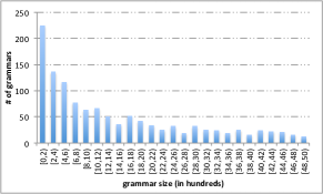
Figure 9: Distribution of grammar sizes in the repository.

Dataset. We implemented a workflow generator that creates a repository containing a mix of recursive and non-recursive grammars, of which some are stand-alone, while others reuse existing workflows as modules. Repository size, workflow characteristics, and the amount of reuse are specified as generator parameters. All experiments in this section were executed with the following parameter settings. A simple workflow has at most 5 modules; a given module has a probability of 0.6 to be composite, and a probability of 0.4 to occur multiple times within the workflow. Each composite module has at most 3 productions, each simple workflow has a probability of $0.5$ to be recursive, and each grammar reuses at most $5$ other grammars.

Using these parameter settings, we generated a repository consisting of about 1,200 grammars. The distribution of grammar sizes in the repository is shown in Figure 9. The size of a grammar ranges from $10$ to $5,000$, and most grammars have size smaller than $1,000$. (Note that grammar size is defined as the total number of symbols in its productions.)

Our choice of parameters is based on our analysis of myExperiment.org, the largest public repository of scientific workflows, and on [31], where it was observed that most current workflows are small.

Next, we generated keyword annotations for the workflows in the repository using results of keyword co-occurrence analysis of [32]. This analysis was based on myExperiment.org, where users tag workflows in support of keyword search. In [32] we used topic mining to extract 20 topics from the repository, with each topic defining a probability distribution over the tags. Here, we take 20 most frequent keywords per topic, and use their probabilities to achieve a realistic keyword assignment to workflow modules. Given a workflow, the repository generator first randomly chooses a topic, and then assigns at most $3$ keywords to each module in accordance with the topic’s probability distribution.

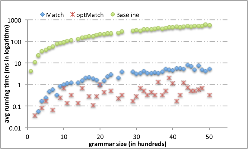
(a) Average running time of $Match$ for $Q_{2}$. Point $(x,y)$ represents running time over grammars of size in $[x-100,x)$.

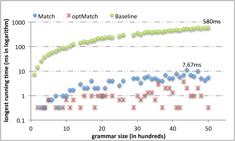
(b) Longest running time $Match$ for $Q_{2}$. Point $(x,y)$ represents running time over grammars of size in $[x-100,x)$.

(c) Improvement of $OptMatch$ over $Match$.

Figure 10: Performance of $Match$ and $OptMatch$.

Queries. We experimented with many different queries, generated by first randomly choosing a topic, and then drawing between 2 and 8 keywords according to the topic’s probability distribution. Due to space constraints, we show only representative results. Unless otherwise noted, all experiments use three queries described below.

$Q_{1}=\{text\;mining,e\mbox{-}lico,workflow\;component\}$ consists of 3 most frequent keywords from its topic, and retrieves workflows with text mining components, contributed by members of $e\mbox{-}lico$ (an e-laboratory for collaborative research). $Q_{2}=\{TerMine,text\;encoding,input\}$ looks for possible inputs to $TerMine$ (a web demonstration service). $Q_{3}=\{input,xml\;invalid,read\;file\}$ is a more technical query. In experiments that focus on scalability, we work with 7 additional queries that contain up to 8 keywords, and where larger queries are supersets of smaller queries.

6.2 Keyword query match

We now evaluate the performance of algorithms described in Section 3. We show that $Match$ (Algorithm 1) runs in time polynomial in the size of the grammar, and that the $OptMatch$ optimization (Algorithm 2) is effective for the vast majority of queries. We then discuss the effectiveness of the sharing optimization (Section 3.3).

We first evaluate the performance of $Match$ compared with the general method that intersects a given grammar $G$ with a query $Q$ represented by a finite state automaton [2] or a graph chain pattern [12]. An adaption of the method to our scenario (called $Baseline$ in Figure 10) works as follows. First, we transform grammar $G$ to grammar $G^{\prime}$, where each production has at most two symbols on the right-hand side. Having the grammar in this form guarantees quadratic data complexity of the algorithm, and is done off-line. Next, we intersect $G^{\prime}$ with $Q$ to construct a new grammar $G^{\prime\prime}$, where 1) for each production $M\rightarrow\alpha_{1}\alpha_{2}$ in $G^{\prime}$, add a production $(M,X)\rightarrow(\alpha_{1},X_{1})(\alpha_{2},X_{2})$ to $G^{\prime\prime}$, for each $X\subseteq Q$, $X_{1}\cup X_{2}=X$, making $(M,X),~{}(\alpha_{1},X_{1}),~{}(\alpha_{2},X_{2})$ symbols in $G^{\prime\prime}$; and 2) for each terminal $M$ in $G^{\prime}$, mark the symbol $(M,\{M\}\cap Q)$ in $G^{\prime\prime}$ as a terminal. Having constructed $G^{\prime\prime}$, the algorithm checks whether its language is empty in time linear in grammar size [19]. $G$ matches $Q$ iff the language of $G^{\prime\prime}$ is not empty.

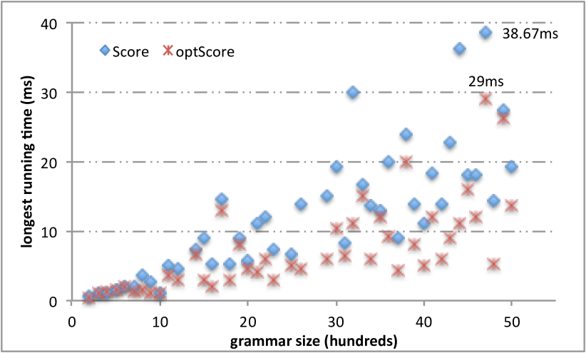
(a) Longest running time of $Score$ and $optScore$ for $Q_{2}$

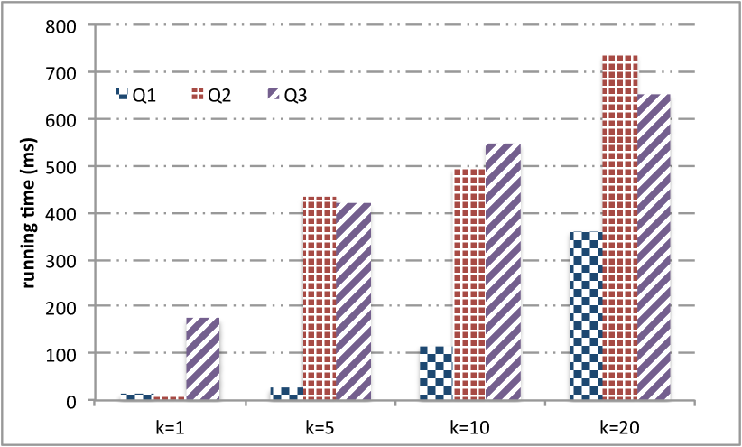
(b) Running time of TA (ms).

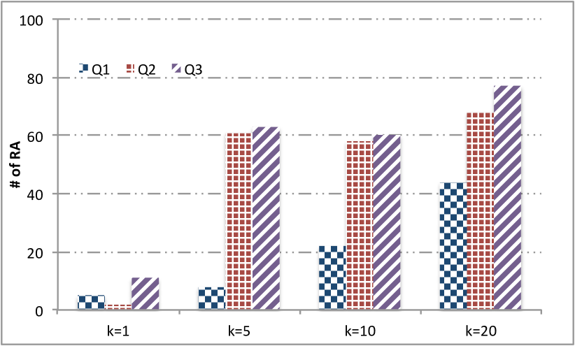
(c) Running time of TA (RA).

Figure 11: Performance of the ranking solution: $Score$, $OptScore$ and threshold algorithm (TA).

(a) $Q_{1}$

(b) $Q_{3}$

(c) Size of the top-1 tree

Figure 12: Performance of finding top-$k$ rpTrees for the top-$10$ grammars (ellipses indicate non-recursive grammars).

Figures 10(a) and 10(b) demonstrate the average and longest running time of $Match$ and $Baseline$ for query $Q_{2}$ for grammars of different sizes. Some 154 grammars in our repository contain all keywords of $Q_{2}$, and we run the algorithms on these grammars. According to Figure 10(a) and 10(b), $Match$ runs in time polynomial in grammar size, as expected. The running time of the algorithm is reasonable, and is below 10ms for all grammars. We observed similar trends for other queries. Although $Baseline$ and $Match$ both run in time polynomial in grammar size, $Match$ significantly outperforms $Baseline$ in all cases, because it terminates early if a variable other than the start symbol matches the query.

Figure 10(c) shows that $OptMatch$, which is an optimization of $Match$, is effective at reducing the running time for most queries. For example, $OptMatch$ outperforms $Match$ by at least 20% for 80% of 2-keyword queries. $OptMatch$ slightly increases running times for some queries. We also measured the total running time of $Match$ and $OptMatch$ for a variety of queries, and for all workflows in the repository. We found that $OptMatch$ brings an over-all gain of at least a factor of 2 for queries of size between 2 and 8. For example, the total running time of $Match$ for queries of size 2 is 77.67ms, compared to 43ms for $OptMatch$.

Finally, we measured the effectiveness of leveraging grammar reuse, when executing $Match$ and $OptMatch$ on all workflows in the repository (see Section 3.3). We found that this optimization, to which we refer as sharing, is extremely effective, bringing the total running time of $Match$ to between 130ms and 150ms for queries of size 2 to 8. Match and OptMatch have comparable performance with this optimization. Details are omitted due to lack of space.

In summary, $Match$ and $OptMatch$ are efficient algorithms. $OptMatch$ outperforms $Match$ for most grammars, and should be used when individual grammars are tested. Either Match or OptMatch with the sharing optimization may be used when all workflows in the repository are tested.

6.3 Ranking of grammars

We now demonstrate that the techniques of Section 4 can be implemented efficiently. We first show that the running time of $Score$ (Algorithm 3) is polynomial in grammar size, and that $OptScore$ outperforms $Score$ in most cases. We then show that top-$k$ workflows can be identified efficiently when TA is used to find the promising grammars.

We observed similar trends for average and longest running time of $Score(optScore)$ to that of $Match(optMatch)$. Figure 11(a) reports the longest running times of $Score$ and $optScore$ for grammars in our repository and demonstrates that the running time of this algorithm is reasonable, and is below 40ms for all grammars. Comparing Figure 11(a) with Figure 10(b), we note that $Score$ is almost three times slower than $Match$. We also observe that our Score algorithm outperforms Baseline [12] (which is used for matching). Since a scoring algorithm is necessarily slower than a matching algorithm, we conclude that a scoring algorithm that uses a similar framework as Baseline will be less efficient than Score, and do not run a direct experimental comparison.

We also measured the improvement of $optScore$ over $Score$ and got a trend very similar to those observed for $OptMatch$ (Figure 10(c)). $OptScore$ results in an improvement for the vast majority of grammars, for queries of varying lengths.

Figure 11(b) reports the running time of Threshold Algorithm (TA), followed by an execution of $OptScore$ for the promising grammars, for queries $Q_{1},Q_{2},Q_{3}$. We can see from Figure 11(b) that it takes under $100ms$ to find the top-5 grammars for $Q_{1}$, and around $400ms$ for $Q_{2}$ and $Q_{3}$. These queries all match between $150$ and $180$ grammars in our repository, and, as is usually the case for TA, the difference in performance is due to the distribution of scores. Figure 11(c) gives the running time of TA in terms of the number of random accesses (RA), demonstrating that the stopping condition for TA is reached after only a fraction of all matching grammars have been considered.

In summary, $Score$ and $OptScore$ are efficient algorithms, and $OptScore$ outperforms $Score$ for most grammars. Using TA to identify promising grammars, and then invoking $OptScore$ for these grammars, allows us to achieve interactive response times when retrieving the top-$k$ grammars from the repository.

6.4 Result presentation

Finally, we evaluate the running time and quality of $topKRep$ (Algorithm 4), and show that it can be used to find the highest-scoring representative parse trees in interactive time.

Recall from Section 5 that $topKRep$ is invoked on a particular grammar, typically one that is among the highest-scoring grammars for a given query, and computes a fixed number of rpTrees for that grammar that match the query.

Figure 12 reports the total running time of $topKRep$ over top-$10$ grammars for queries $Q_{1}$ and $Q_{3}$, as a function of grammar size. The number of rpTrees, denoted $k$, varies from 1 to 10. Observe from Figure 12(a) that the top-$10$ grammars for $Q_{1}$ are small $(<200)$, and that the total running time of $topKRep$ is reasonable, under $161.33ms$ for $k=10$.

We use ellipses to indicate running times for non-recursive grammars. We noted in Section 5 that, because all parse trees of non-recursive grammars are representative, we can design an efficient version of $topKRep$ for this case. The difference in running time is not significant for $Q_{1}$ (Figure 12(a)), but becomes more pronounced for $Q_{3}$ (Figure 12(b)).

Figure 12(b) shows that $topKRep$ is significantly slower for $Q_{3}$ than for $Q_{1}$, for three reasons. First, the top-10 grammars for $Q_{3}$ are much larger, and have larger parse trees. Figure 12(c) shows that sizes of top-1 trees for large grammars are usually larger than those for small grammars. Second, there are more parse trees to be constructed for large grammars. Third, it is more common for large grammars to require a larger buffer size when computing the top-$k$ rpTrees. Recall that buffer size is an argument in Algorithm 4, and that the algorithm is re-executed with a larger buffer if the original setting does not yield enough rpTrees. For the $4^{th}$ grammar in Figure 12(b), the required buffer size for $k=3$ was $48$ (meaning that $topKRep$ was executed 5 times). This was higher than for $k=5$ and $k=10$, where buffer size of 40 (for 4 and 3 executions of $topKRep$, respectively) was sufficient.

We now present an example that illustrates the effectiveness of rpTrees. For query $Q_{1}$, the top-1 matching grammar in our repository is one where the start module is annotated with all the keywords in $Q_{1}$. Thus all parse trees of this grammar match $Q_{1}$. To simplify presentation, we eliminate the keywords of modules and show only the grammar below:

$r_{1}:S\Rightarrow\{S,B\}~{}(\frac{1}{3})$	$r_{2}:S\Rightarrow\{A,A,S,s_{1}\}~{}(\frac{1}{3})$
$r_{3}:S\Rightarrow\{s_{2}\}~{}(\frac{1}{3})$	$r_{4}:A\Rightarrow\{B,a_{1}\}~{}(\frac{1}{2})$
$r_{5}:A\Rightarrow\{a_{2}\}~{}(\frac{1}{2})$	$r_{6}:B\Rightarrow\{S,b_{1}\}~{}(\frac{1}{3})$
$r_{7}:B\Rightarrow\{S,b_{2}\}~{}(\frac{1}{3})$	$r_{8}:B\Rightarrow\{b_{3}\}~{}(\frac{1}{3})$

Note that the top-6 trees of this grammar are all rpTrees. The $7^{th}$ most probable tree $T_{7}$ (with a probability $0.004$) is shown in Figure 13(b). Observe that $T_{7}$ is subsumed by the top $2^{nd}$ tree $T_{2}$ (Figure 13(a)), and so is not an rpTree. On the other hand, $T_{8}$ (with probability $0.003$) is an rpTree, and is more interesting to show to the user than $T_{7}$, although its probability score is lower.

(a) top-$2$ tree

(b) top-$7$ tree

(c) top-$8$ tree

Figure 13: Trees for the top-1 grammar that matches $Q_{1}$

In summary, $topKRep$ can be used to efficiently compute the highest-scoring representative parse trees for many grammars. For certain large grammars, $topKRep$ does not terminate in interactive time, due to parse tree size, and to conservative buffer size requirements. Performance can be improved using alternative strategies for setting buffer size.

7 Conclusions

In this paper we addressed the problem of searching a repository of workflow specifications in which modules, both atomic and composite, are annotated with keywords. Since search does not interact with the graph structure of workflows, we reduced the problem to one of searching a repository of bag grammars. We gave an efficient polynomial-time matching algorithm with respect to data complexity, and extended this to search over a repository of bag grammars. We developed efficient algorithms for calculating the relevance score of a grammar to a given query, and for finding the top-$k$ grammars for a given query. Finally, we proposed a novel result presentation method.

This work introduces a novel use of bag grammars, and shows the importance of probabilistic bag grammars. Our approach has been based on efficiency considerations; in the future we would like to gain a deeper understanding of how to use probabilistic bag grammars and continue to explore ways of presenting concise search results. Moving beyond keyword search, we would like to add structural features into queries. We also plan on testing the usability of these ideas on real datasets.

8 Acknowledgements

We thank Tova Milo for extensive discussions and feedback on this draft.

References

- [1] Z. Bao et al. Labeling recursive workflow executions on-the-fly. In SIGMOD, 2011.
- [2] Y. Bar-Hillel et al. On formal properties of simple phrase structure grammars. Language and Information: Selected Essays on Their Theory and Application, 1964.
- [3] C. Beeri et al. Querying business processes. In VLDB, 2006.
- [4] S. P. Callahan et al. Managing the evolution of dataflows with VisTrails. In SciFlow, 2006.
- [5] Y. Chen et al. Keyword search on structured and semi-structured data. In SIGMOD, 2009.
- [6] Z. Chi. Statistical properties of probabilistic context-free grammars. Computational Linguistics, 25, 1999.
- [7] D. Chiu et al. Keyword search support for automating scientific workflow composition. In SSDBM, 2011.
- [8] S. Crespi-Reghizzi and D. Mandrioli. Petri nets and commutative grammars. 74–5, Mar, 1974.
- [9] B. B. Dalvi et al. Keyword search on external memory data graphs. PVLDB, 2008.
- [10] S. B. Davidson et al. Keyword search in workflow repositories with access control. In AMW, 2011.
- [11] D. Deutch et al. Optimal top-k query evaluation for weighted business processes. PVLDB, 3(1), 2010.
- [12] D. Deutch and T. Milo. A structural/temporal query language for business processes. J. Comput. Syst. Sci., 78(2), 2012.
- [13] J. Esparza. Petri nets, commutative context-free grammars, and basic parallel processes, 1997.
- [14] J. Esparza and M. Nielsen. Decidability issues for petri nets - a survey, 1994.
- [15] K. Etessami and M. Yannakakis. Recursive markov chains, stochastic grammars, and monotone systems of nonlinear equations. J. ACM, 56, 2009.
- [16] R. Fagin et al. Optimal aggregation algorithms for middleware. In PODS, 2001.
- [17] A. Gándara et al. Knowledge annotations in scientific workflows: An implementation in kepler. In SSDBM, 2011.
- [18] H. He et al. Blinks: ranked keyword searches on graphs. In SIGMOD, 2007.
- [19] J. E. Hopcroft et al. Introduction to automata theory, languages, and computation. Addison-Wesley, 2003.
- [20] V. Kacholia et al. Bidirectional expansion for keyword search on graph databases. In VLDB, 2005.
- [21] R. M. Karp and R. E. Miller. Parallel program schemata. J. of CSS, 3(2), 1969.
- [22] J. Kleinberg and E. Tardos. Algorithm Design. 2005.
- [23] J. Li et al. Top-k keyword search over probabilistic xml data. In ICDE, 2011.
- [24] Z. Liu and Y. Chen. Processing keyword search on xml: a survey. WWW, 14(5-6), 2011.
- [25] Z. Liu et al. Searching workflows with hierarchical views. PVLDB, 3(1-2), 2010.
- [26] C. D. Manning and H. Schütze. Foundations of statistical natural language processing. MIT Press, 2001.
- [27] A. Nierman and H. V. Jagadish. Protdb: Probabilistic data in xml. In VLDB, 2002.
- [28] T. Oinn et al. Taverna: a tool for the composition and enactment of bioinformatics workflows. Bioinformatics, 20(1), 2003.
- [29] D. D. Roure et al. The design and realisation of the myExperiment virtual research environment for social sharing of workflows. FGCS, 25(5), 2009.
- [30] Q. Shao et al. Wise: A workflow information search engine. In ICDE, 2009.
- [31] J. Starlinger et al. (re)use in public scientific workflow repositories. In SSDBM, 2012.
- [32] J. Stoyanovich et al. Exploring repositories of scientific workflows. In WANDS, 2010.
- [33] J. Stoyanovich and I. Pe’er. Mutagenesys: estimating individual disease susceptibility based on genome-wide snp array data. Bioinformatics, 24(3):440–442, 2008.
- [34] T. Tran et al. Top-k exploration of query candidates for efficient keyword search on graph-shaped (rdf) data. In ICDE, 2009.
- [35] J. X. Yu et al. Keyword search in relational databases: A survey. IEEE Data Eng. Bull., 33(1), 2010.