A Model for Stock Returns and Volatility

Abstract

We prove that Student’s t-distribution provides one of the better fits to returns of S&P component stocks and the generalized inverse gamma distribution best fits VIX and VXO volatility data. We further argue that a more accurate measure of the volatility may be possible based on the fact that stock returns can be understood as the product distribution of the volatility and normal distributions. We find Brown noise in VIX and VXO time series and explain the mean and the variance of the relaxation times on approach to the steady-state distribution.

I Introduction

The generalized inverse gamma (GIGa) function (Appendix A) belongs to a family of distributions (Appendix B), which includes inverse gamma (IGa), lognormal (LN), gamma (Ga) and generalized gamma (GGa). The remarkable property of GIGa is its power-law tail; for a general three-parameter case, the power-law exponent is given by the negative $1+\alpha\gamma$, so that $\text{GIGa}(x;\alpha,\beta,\gamma)\propto x^{-1-\alpha\gamma}$, $x\rightarrow\infty$. GIGa emerges as a steady state distribution in a number of problems, from a network model of economy, ma2013distribution to ontogenetic mass growth, west2012 to response times in human cognition. ma12RT This common feature can be traced to a birth-death phenomenological model subject to stochastic perturbations (Appendix C). Here we argue that the GIGa distribution best describes stock volatility distribution and the product distribution (Appendix D) of GIGa and normal (N) distributions, GIGa*N, best describes stock returns distribution.

Numerically, we used the maximum likelihood method to determine the best parameters for each of the distributions in the above family of distributions and found that GIGa provides the best fit for VIX and VXO volatility data. We also found that among product distributions of the above family with normal distribution, GIGa’s product with N gives the best fit to the stock returns distribution. Furthermore, among the better GIGa*N fits are those with $\gamma\approx 2$.

In general, product distribution GIGa*N has $|x|^{-1-\alpha\gamma}$ tails [left and right]. For $\gamma=2$, the product distribution $\text{GIGa}(\alpha,\beta,2)*\text{N}$ for stock returns is Student’s t-distibution, which has $|x|^{-1-2\alpha}$ tails. praetz1972 ; platen2008 ; gerig2009 . Accordingly, our starting point is the geometric Brownian motion model of stock price, hull1997 ; gatheral2006 where the steady-state distribution of stock returns is given by the product distribution of volatility and normal distributions. Further, the instantaneous variance of volatility (or square stochastic volatility - the terms used interchangeably) is described by the Nelson diffusion limit (NDL) of GARCH$(1,1)$ model of stock volatility nelson1990 ; duan1995 , whose stochastic term is uncorrelated from that in the equation for stock price; in the steady state, it is distributed as IGa, that is GIGa with $\gamma=1$.

This paper is organized as follows. In Sec. II, we discuss stochastic stock and volatility models. In Sec. III, we fit VIX and VXO, including direct evaluation of their power law tail exponents by log-log plot. We also address Brown noise observed in the VIX/VXO time series. In Sec. IV, we discuss numerical results of fitting returns of S&P component stocks based on log-likelihood and discuss white noise in stock return series. In Sec. V, we summarize our key findings.

II Stochastic stock and volatility models

The widely accepted equation for stock price is given by

$$\frac{dS}{S}=\mu dt+\sigma dW_{1}.$$ (1)

where $\mu$ is a constant and $\sigma$ volatility. The equation for the instantaneous volatility variance (square volatility) can be written in the following general form:

$$dV=\tilde{f}(V)dt+\tilde{g}(V)dW_{2}.$$ (2)

Here $dW_{1}$ and $dW_{2}$ are Wiener processes correlated by $\langle dW_{1}dW_{2}\rangle=\rho dt$. Substituting $V=\sigma^{2}$ and using Ito calculus, we obtain the volatility equation

$$d\sigma=f(\sigma)dt+g(\sigma)dW_{2}.$$ (3)

The Fokker-Planck equation for the distribution function of $\sigma$, $P(\sigma,t)$, is given by

$$\frac{\partial}{\partial t}P(\sigma,t)=\frac{1}{2}\frac{\partial^{2}}{\partial\sigma^{2}}[g^{2}(\sigma)P(\sigma,t)]-\frac{\partial}{\partial\sigma}[f(\sigma)P(\sigma,t)].$$ (4)

It has a stationary (steady-state) solution given by

$$P(\sigma)=\frac{2}{g^{2}}\exp({\int\frac{2f}{g^{2}}d\sigma}).$$ (5)

In what follows, we shall assume that $dW_{1}$ and $dW_{2}$ are uncorrelated, that is $\rho=0$. A number of possible forms of $f(\sigma)$ and $g(\sigma)$ are discussed in Appendix E; see also wiggins1987 . Here we concentrate on one particular form

$$d\sigma=J(\theta\sigma^{1-\gamma}-\sigma)dt+\Sigma\sigma dW_{2},$$ (6)

The stationary (see Appendix F for discussion of relaxation times) solution of this equation is given by

$$\begin{split}P(\sigma)&=\text{GIGa}(\sigma;\alpha,\beta,\gamma)\\ &=\text{GIGa}\left(\sigma;\left(1+\frac{2J}{\Sigma^{2}}\right)\gamma^{-1},\left({\theta}\frac{2J}{{\Sigma^{2}}}\gamma^{-1}\right)^{1/\gamma},\gamma\right),\end{split}$$ (7)

where the parameter $\theta$ can be expressed using the mean $\overline{\sigma}$ as

$$\theta=\frac{\gamma\Sigma^{2}}{2J}\left[\frac{\overline{\sigma}\Gamma((1+\frac{2J}{\Sigma^{2}})\gamma^{-1})}{\Gamma(\frac{2J}{\Sigma^{2}}\gamma^{-1})}\right]^{\gamma}.$$ (8)

In particular, when $\gamma=1$, $\theta=\overline{\sigma}$.

A case of particular importance is $\gamma=2$, in which case the equation for the volatility variance is that of $\gamma=1$ and reads as follows:

$$dV=\tilde{J}(\overline{V}-V)dt+\tilde{\Sigma}VdW_{2}.$$ (9)

Its stationary solution is given by the IGa distribution,

$$P(V)=\text{IGa}\left(V;1+\frac{2\tilde{J}}{\tilde{\Sigma}^{2}},\overline{V}\frac{2\tilde{J}}{\tilde{\Sigma}^{2}}\right).$$ (10)

Using $V=\sigma^{2}$ and Ito calculus, we obtain

$$d\sigma=\left(\frac{\tilde{J}}{2}\overline{V}\sigma^{-1}-\left(\frac{\tilde{J}}{2}+\frac{\tilde{\Sigma}^{2}}{8}\right)\sigma\right)dt+\frac{\tilde{\Sigma}}{2}\sigma dW_{2}.$$ (11)

On comparison with Eq. (6), we find the following parameter correspondence:

$$\begin{split}&J=\frac{\tilde{J}}{2}+\frac{\tilde{\Sigma}^{2}}{8}\\ &\theta=\overline{V}\frac{\tilde{J}}{2}\left(\frac{\tilde{J}}{2}+\frac{\tilde{\Sigma}^{2}}{8}\right)^{-1}\\ &\Sigma=\frac{\tilde{\Sigma}}{2}\\ &\gamma=2.\end{split}$$ (12)

Substitution into Eq. (7), gives the distribution of $\sigma$ as,

$$\text{GIGa}\left(\sigma;1+\frac{2\tilde{J}}{\tilde{\Sigma}^{2}},\sqrt{\overline{V}\frac{2\tilde{J}}{\tilde{\Sigma}^{2}}},2\right),$$ (13)

It should be emphasized that a simple change of the variate to its square root produces the following transformation: $\text{GIGa}(\alpha,\beta,\gamma)\rightarrow\text{GIGa}(\alpha,\sqrt{\beta},2\gamma)$ and in particular $\text{IGa}(\alpha,\beta,1)\rightarrow\text{GIGa}(\alpha,\sqrt{\beta},2)$, which is consistent with (9) and (13). From (8), the mean of $\sigma$ is given by

$$\sqrt{\overline{V}}\sqrt{\frac{2\tilde{J}}{\tilde{\Sigma}^{2}}}\frac{\Gamma\left(\frac{2\tilde{J}}{\tilde{\Sigma}^{2}}+\frac{1}{2}\right)}{\Gamma\left(\frac{2\tilde{J}}{\tilde{\Sigma}^{2}}+1\right)},$$ (14)

which is a monotonically increasing function which approaches $\sqrt{\overline{V}}$ as $2\tilde{J}/\tilde{\Sigma}^{2}\rightarrow\infty$.

Turning to Eq. (1), we observe that the stationary distribution of stock returns is a product distribution $P(\sigma)*\text{N}$. In Appendix D, we consider both formalism of the product distribution and various cases of $P(\sigma)$. Here we concentrate specifically on

$$\text{GIGa}(\alpha,\beta,2)*\text{N}(0,1)=\frac{\Gamma\left(\frac{1}{2}+\alpha\right)}{\sqrt{2\pi}\beta\Gamma(\alpha)}\left(\frac{2\beta^{2}}{z^{2}+2\beta^{2}}\right)^{\frac{1}{2}+\alpha},$$ (15)

which is the generalized Student’s t-distribution T$(0,{\beta}/{\sqrt{\alpha}},2\alpha)$ jackman2009 .

It should be mentioned that by Ito calculus and Eq. (1)

$$d\log S=(\mu-\frac{1}{2}\sigma^{2})dt+\sigma dW_{1}.$$ (16)

In numerical calculations of stock returns, it is actually the $\Delta\log S$ that is being evaluated. However, it is clear that the premise of the stationary distribution being the product distribution of the volatility distribution and the normal distribution remains in force.

III Market volatility

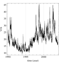
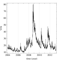
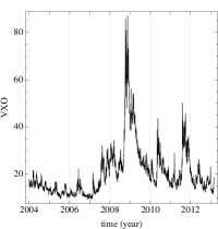
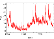
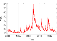
We analyze the Chicago Board Options Exchange (CBOE) volatility index CBOE_website ; VIX_CBOE ; VXO_CBOE . On September 22, 2003, CBOE decided to change the manner in which it calculated the volatility index from VXO to VIX. However, both methods were applied to both the old and new data. Following CBOE convention CBOE_website , the VIX/VXO data from 1990 to 2004 are called vixarchive/vxoarchive and from 2004 to present vixcurrent/vxocurrent. In Fig. 1, we show the time series of the indices.

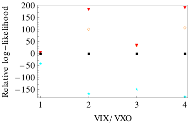
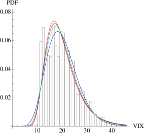
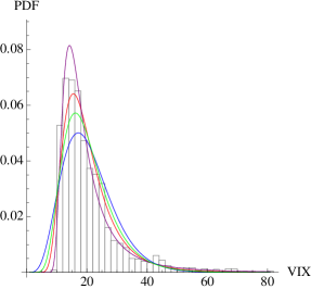
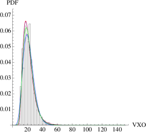
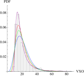
We apply the maximum likelihood estimation method (Appendix G) to find the best fitting parameters of IGa, GIGa, Ga, and LN summarized in Table 1. Comparison of loglikelihood in Fig. 2 shows that the goodness of fit decreases in the following order: GIGa, IGa, LN, and Ga.

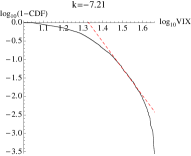
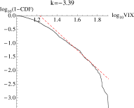
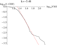
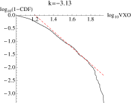
In Fig. 3, we plot histograms of vixarchive, vixcurrent, vxoarchive, and vxocurrent respectively, fitted with the best GIGa, IGa, LN, and Ga. We also measure the exponent of the power law tail of VIX and VXO directly (Apendix H), as shown in Fig. 4 and Table 2.

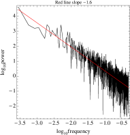
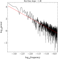
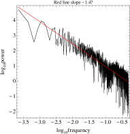
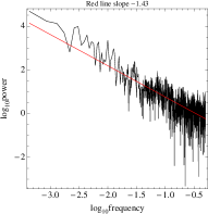
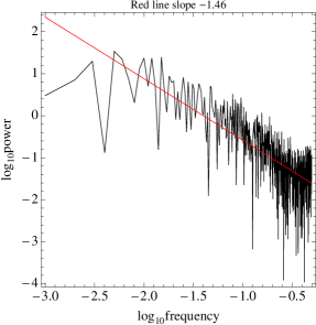
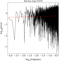
Finally, in Fig. 5 we clearly observe Brown noise in the volatility time series. This is entirely consistent with the Brown noise observed in the time series of the GIGa process of Eq. (6); in Fig. 6 we show Brown noise for an IGa process, $\gamma=1$.

Figure 1: VIX and VXO plots.

Data	IGa: $\alpha,\beta$	GIGa: $\alpha,\beta,\gamma$	LN: $\mu,\sigma$
vixarchive	$10.7,196$	$33.7,1.03\times 10^{4},0.557$	$2.96,0.311$
vixcurrent	$7.22,127$	$0.721,14.1,3.96$	$2.94,0.398$
vxoarchive	$9.63,187$	$11.7,295,0.905$	$3.02,0.330$
vxocurrent	$6.59,113$	$0.678,13.4,3.94$	$2.92,0.419$

Table 1: Parameters of fitting distributions.

Figure 2: Log-likelihood of fitting distribtuion relative to LN. Red down-pointing triangles: GIGa; orange diamonds: IGa; cyan stars: Ga; and black squares: LN. 1 at the x-axis is for vixarchive, 2 for vixcurrent, 3 for vxoarchive, and 4 for vxocurrent.

Figure 3: Histogram plots of VIX and VXO. Top down: vixarchive, vixcurrent, vxoarchive, and vxocurrent. Red: IGa; purple: GIGa; blue: Ga; and green: LN.

Figure 4: Log-log plots of VIX and VXO. Black curves: log-log plots; red dashed lines: linear fit of the log-log plots from $1-CDF=0.01$ to $0.1$.

Data	IGa: $-\alpha$	GIGa: $-\alpha\gamma$	Slope of log-log plot
vixarchive	-10.7	-18.8	-7.21
vixcurrent	-7.22	-2.86	-3.39
vxoarchive	-9.63	-10.6	-5.48
vxocurrent	-6.59	-2.67	-3.13

Table 2: Power-law tail exponents of fitting distributions and log-log plot.

Figure 5: Fourier transform of VIX and VXO time series. Jagged black lines: discrete Fourier transform; red lines: linear fit of the black lines.

Figure 6: Discrete Fourier transform of a time series of IGa process with $J=0.1$, $\sigma=\sqrt{0.1}$ at time 1, 2, …, 1000. Jagged black line: discrete Fourier transform; red line: linear fit of the black lines.

IV Stock returns

We analyze component stock prices (at close) of major indices. S&P 100 and S&P 500 lists can be found at the Standard & Poor’s website.SP_website The historical daily prices of component stocks of S&P 100 and S&P 500 are downloaded from Yahoo! Finance.YahooFinance_website The final date of S&P 100 and S&P 500 stocks used here is March 25, 2013. The daily S&P 500 and DJIA data is downloaded from the Research Division of the Federal Reserve Bank of St. Louis.FedStLouis_website1 ; FedStLouis_website2 For S&P 500, we ignored five stocks that have less than 200 stock datapoints each.

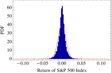
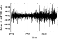
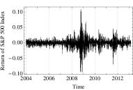
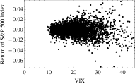
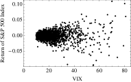
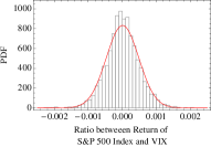
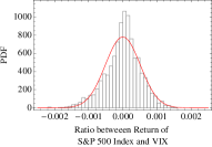
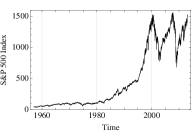
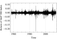
We start with a simple test of the stochastic volatility model, Eqs. (1) and (6). In Fig. 7, we show stock returns of S&P 500 index and their distribution. Average daily return, $\log(S_{tomorrow})-\log(S_{today})\approx(S_{tomorrow}-S_{today})/S_{today}\approx 0.00025$ corresponds to 6.4% annual return. For constant volatility, one would expect a normal distribution for stock returns. However, as is obvious from the figure, normal distribution is not a good fit. On the other hand, the stochastic volatility model indicates that it is the ratio of stock return to volatility that should be normal. Visual inspection of Fig. 8 and the fit in Fig. 9 give initial validation to the model.

Figure 7: Top left: historical curve of daily S&P 500 index. Top right: historical curve of daily return of S&P 500 index. Bottom: histogram of return of S&P 500 index. The red line is a fit of normal distribution. In the plots, return is computed from $\log S_{tomorrow}-\log S_{today}$ without other operations.

Figure 8: Left three plots: return and VIX from 01/02/1990 to 12/31/2003. Right three plots: return and VIX from 01/02/2004 to 02/26/2013.

Figure 9: Ratio of return and VIX. Left: from 01/02/1990 to 12/31/2003. Right: from 01/02/2004 to 02/26/2013.

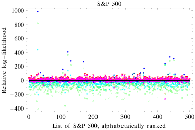
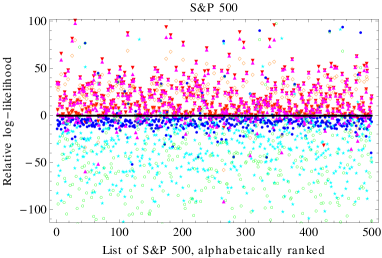
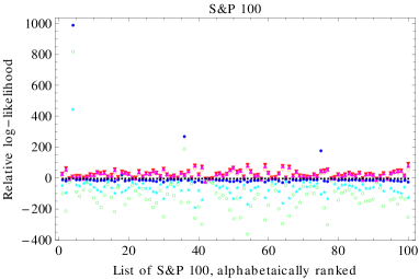
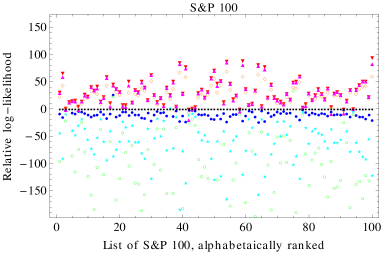
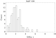
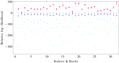
We proceed to rigorously analyze stock returns data using maximum likelihood estimation. In our analysis, the stock returns are detrended and scaled into unit STDEV. The log-likelihood of product distribution is evaluated by numerical quadrature and maximized by the simplex algorithm. The numerical quadrature and the simplex algorithm are checked to be correct for the special case $\text{GIGa}(\alpha,\beta,2)*N$, which is generalized Student’s t-distribution, whose maximum likelihood estimation can be computed directly. MaThesis2013 Figs. 10-12 convincingly show that the product distribution $\text{GIGa}(\alpha,\beta,\gamma)*\text{N(0,1)}$ fits the stock return best. Distributions of best fit parameters are shown in Figs. 13 and 14.

Figure 10: Log-likelihood of DJIA, S&P 500 index, and DJIA component stocks. From 1 to 32, the $x$-coordinates correspond to DJIA, S&P 500 index, AA, AXP, BA, BAC, CAT, CSCO, CVX, DD, DIS, GE, HD, HPQ, IBM, INTC, JNJ, JPM, KO, MCD, MMM, MRK, MSFT, PFE, PG, T, TRV, UNH, UTX, VZ, WMT, and XOM. All the values of log-likelihood are relative to the LN distribution. Red down-pointing triangles: GIGa*N, magenta up-pointing triangles: GIGa$(\alpha,\beta,2)$*N, orange diamonds: IGa*N, black squares: LN*N, blue dots: GGa*N computed from the simplex method with iteration numbers as 1000, cyan stars: Ga*N, and green circles: GGa$(\alpha,\beta,2)$*N. The parameter $\alpha\gamma$ of GIGa (Red) is 3.79, 5.99, 3.35, 3.61, 3.7, 2.5, 3.76, 2.92, 3.58, 3.78, 3.4, 3.02, 3.16, 3.28, 3.13, 3.01, 3.72, 3.63, 3.13, 2.91, 3.84, 3.2, 2.95, 3.38, 3.37, 3.95, 3.23, 2.97, 3.93, 3.76, 3.17, 3.21. The parameter $\gamma$ of GIGa (Red) is 1.17, 0.69, 2.32, 1.64, 2.11, 1.6, 1.89, 2.6, 2.89, 1.89, 2.23, 2.9, 2.53, 2.66, 2.68, 4.3, 1.93, 1.17, 2.63, 4.27, 1.76, 3.59, 2.49, 3.02, 2.17, 1.36, 1.6, 2.24, 1.86, 1.67, 2.08, 5.36.

Figure 11: Log-likelikelood of S&P 500. All the values of log-likelihood are relative to the LN distribution. Red down-pointing triangles: GIGa*N, magenta up-pointing triangles: GIGa$(\alpha,\beta,2)$*N, orange diamonds: IGa*N, black squares: LN*N, blue dots: GGa*N computed from the simplex method with iteration numbers as 1000, cyan stars: Ga*N, and green circles: GGa$(\alpha,\beta,2)$*N. Top plot for all the range of log-likelihood and bottom plot for a shorter range.

Figure 12: Log-likelikelood of S&P 100. All the values of log-likelihood are relative to the LN distribution. Red down-pointing triangles: GIGa*N, magenta up-pointing triangles: GIGa$(\alpha,\beta,2)$*N, orange diamonds: IGa*N, black squares: LN*N, blue dots: GGa*N computed from the simplex method with iteration numbers as 1000, cyan stars: Ga*N, and green circles: GGa$(\alpha,\beta,2)$*N. Top plot for all the range of log-likelihood and bottom plot for a shorter range.

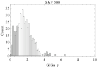
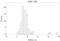
Figure 13: Parameters of GIGa used in fitting S&P 500 (top) and S&P 500 (bottom). $\alpha\gamma$ is the thereotical exponent of the power-law tails in stock return. $\gamma$ is the control parameter. If $\gamma=2$, the volatility variance is described by IGa, which can be generated by a mean-field theory of (9). Bouchaud2000 ; ma2013distribution The mean of $\alpha\gamma$ is 4.3 and the median is 3.6. The mean of $\gamma$ is 1.9 and the median is 1.5 for S&P 500 and 2.1 and 2.0 for S&P 100.

Figure 14: Parameter $\alpha$ of GIGa$(\alpha,\beta,2)$ used in fitting S&P 500 (left) and S&P 100 (right). $2\alpha$ is the theoretical exponent of the power-law tails in stock return. The mean of $2\alpha$ is 3.2 and the median is 3.1 for S&P 500 and 3.3 and 3.4 for S&P 100.

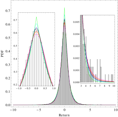
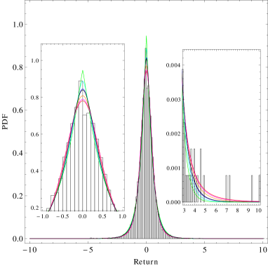
In Fig. 15, we show histograms of S&P 500 index and IBM respectively and their fitting by product distributions. Clearly, the product distribution of GIGa and normal distribution is better able to capture the tail events.

Figure 15: Fitting of stock return rate of S&P 500 (top) and IBM (bottom). Red: GIGa*N, magenta: GIGa$(\alpha,\beta,2)$*N (Student’s t-distribution), orange: IGa*N, black: LN*N, blue: GGa*N computed from the simplex method with iteration numbers as 1000, cyan: Ga*N, and green: GGa$(\alpha,\beta,2)$*N.

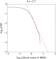
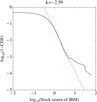
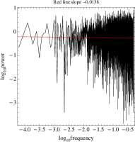
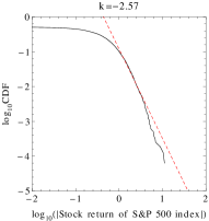
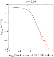
In Figs. 16 and 17, we do direct fitting of tails of stock return of S&P 500 index and IBM respectively (Appendix H). Obviously the stock return is fat-tailed. However, the tail exponents obtained here deviate from those obtained by GIGa*N fitting in Fig. 10. In Fig. 18, we show the Fourier transform of stock return series of S&P 500 index and IBM respectively. It exhibits white noise as opposed to the Brown noise of VIX and VXO in Fig. 5.

Figure 16: Log-log plot of stock return rate of S&P 500. Left: the left tail of negative stock return. The $x$-axis is logarithm of absolute values of stock return and the $y$-axis is CDF. Right: the right tail of (positive) stock return.

Figure 17: Log-log plot of stock return rate of IBM. Left: the left tail of negative stock return. The $x$-axis is logarithm of absolute values of stock return and the $y$-axis is CDF. Right: the right tail of (positive) stock return.

Figure 18: Fourier transform of stock return of S&P 500 (left) and IBM (right).

Notice that in the Heston model heston1993 ; gatheral2006 (Appendix E) stock returns are given by GGa$(\alpha,\beta,2)*\text{N(0,1)}$ and cannot generate power-law tail. This contradicts both our and previous results Stanley1996 ; Cizeau1997 ; Liu1999 ; Gopikrishnan1999 ; Plerou1999 of $\approx$ 3 to 5 for the tail exponent.

V Summary

We demonstrated that that $\text{GIGa}(\alpha,\beta,\gamma)$ provides the best fit to volatility distribution and the product distribution $\text{GIGa}(\alpha,\beta,\gamma)*\text{N(0,1)}$ to stock return distribution. Furthermore, we showed that $\gamma=2$ is near the median/mode of the $\gamma$-distribution of best fits. For $\gamma=2$, the stock return distribution is the generalized Student’s t-distribution T$(0,{\beta}/{\sqrt{\alpha}},2\alpha)$. Numerical evaluation of parameters of fitting distributions was done with the maximum likelihood estimation method.

Importance of $\gamma=2$ puts our findings in excellent agreement with the stochastic volatility and stock return model defined by Eqs. (1) and (6). This model fully accounts for the power law tails observed in the volatility and stock return distributions. Additional evidence comes from the fact that Fourier transform of both empirical and simulated time series exhibit Brown noise for volatility and white noise for stock returns (volatility couples to Wiener noise in (1) while stock return in (6) does not, which accounts for the difference).

Lastly we argue that since the stock returns have been accumulated over much longer period of time and the definitions of VIX and VXO have changed over time, a better definition of a steady-state volatility would be a distribution whose product with the normal distribution gives distribution of stock returns. This, in turn, may lead to a better approach to calculating volatility than the currently adopted standard.

Appendix A Properties of GIGa distribution

We begin with the $\gamma=1$ limit of GIGa, namely IGa distribution PDF

$$P_{\text{IGa}}(x)=\frac{1}{\beta\Gamma(\alpha)}\exp\left[-\frac{\beta}{x}\right]\left(\frac{\beta}{x}\right)^{1+\alpha}.$$ (17)

Setting the mean to unity, the scaled distribution is

$$P_{\text{IGa}}^{\text{Scaled}}(x)=\frac{(\alpha-1)^{\alpha}\exp\left(-\frac{\alpha-1}{x}\right)}{\Gamma(\alpha)x^{1+\alpha}}.$$ (18)

The mode of the above distribution is $x_{\text{mode}}=(\alpha-1)/(\alpha+1)$. The modal PDF is

$$P_{\text{IGa}}^{\text{Scaled}}(x_{\text{mode}})=\frac{(1+\alpha)^{1+\alpha}\exp(-1-\alpha)}{\Gamma(\alpha)(\alpha-1)},$$ (19)

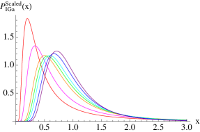
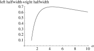
which has a minimum at $\alpha\approx 3.48$ as shown in Fig. 19. The change in PDF behavior on transition through this value is clearly observed Fig. 20. Also plotted in Fig. 19 is the half-width of the distribution. Clearly, it highly correlates with the modal PDF above.

Figure 19: Mode and half-width of scaled IGA as a function of $\alpha$

Figure 20: PDF of IGa distributions. From left to right, $\alpha=1.5,2,3,3.48,4,5$, and $6$, corresponding to red, magenta, orange, green, cyan, blue, and purple lines.

Both minimum and maximum above clearly separate the regime of small $\alpha$: $\alpha\rightarrow 1$, where the approximate form of the scaled PDF is

$$P_{\text{IGa}}^{\text{Scaled}}(x)\approx\frac{(\alpha-1)\exp\left[-\frac{\alpha-1}{x}\right]}{x^{2}},$$ (20)

whose mode is $(\alpha-1)/2$ and the magnitude of the maximum is $4\exp[-(\alpha-1)^{2}/2]/(\alpha-1)\approx 4/(\alpha-1)$, from the regime of large $\alpha$, $\alpha\rightarrow\infty$, where

$$P_{\text{IGa}}^{\text{Scaled}}(x)\rightarrow\delta(x-1).$$ (21)

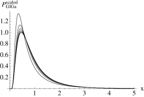
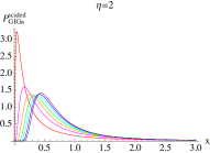
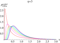
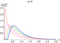
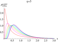
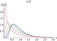
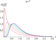
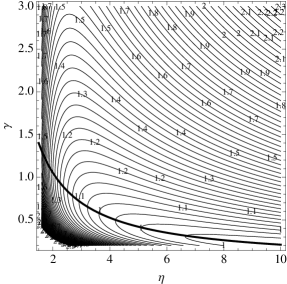
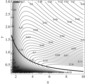
We now turn to GIGa distribution and the effect of parameter $\gamma$. In Fig. 21 we give the contour plots of modal PDF and total half-widths in the $(\eta,\gamma)$ plane, where $\eta=\alpha\gamma$ and $-1-\eta$ is the exponent of the power law tail. We observe an interesting scaling property of GIGa: for $\gamma\approx 2.1/\eta$, the dependence of the PDF on $\eta$ is very weak, as demonstrated in Fig.22, where it is plotted for integer $\eta$ from 2 to 7. An alternative way to illustrate this is to plot PDF for a fixed $\eta$ and variable $\gamma$, as shown in Fig. 23. Following the thick line we notice that, for $\eta>3$, mode and half-width change very little with $\eta$. The key implication of the scaling property is that IGa contains all essential features pertinent to GIGa.

Figure 21: Top: contours of modal PDF of GIGa distributions with mean $1$. Thin lines: contours of modal PDF at mode. Thick line: $\gamma=2.1/\eta$. Bottom: contours of total half-widths of GIGa distributions with mean $1$. Thick line: $\gamma=2.5/\eta$.

Figure 22: Scaled PDF of GIGa distributions with mean $1$. In the plots, $\gamma=2.1/\eta$. Six lines correspond to $\eta=2,3,...,7$

Figure 23: Scaled PDF of GIGa distributions with mean $1$. In each subplot with constant $\eta$, from left to right, $\gamma=0.5/\eta,1/\eta,1.5/\eta,2/\eta,2.5/\eta,3/\eta$, and $3.5/\eta$, corresponding to red, magenta, orange, green, cyan, blue, and purple lines.

Appendix B Parametrization of the GIGa family of distributions

This Appendix is a self-contained re-derivation of a LN limit of GIGa. weibullcom The three-parameter GIGa distribution is given by

$$\text{GIGa}(x;\alpha,\beta,\gamma)=\frac{\gamma}{\beta\Gamma(\alpha)}e^{-\left(\frac{\beta}{x}\right)^{\gamma}}\left(\frac{\beta}{x}\right)^{1+\alpha\gamma}$$ (22)

for $x>0$ and 0 otherwise. We require that $\alpha,\beta,\gamma>0$. IGa is the the $\gamma=1$ case of GIGa:

$$\text{IGa}(x;\alpha,\beta)=\frac{1}{\beta\Gamma(\alpha)}e^{-\frac{\beta}{x}}\left(\frac{\beta}{x}\right)^{1+\alpha}.$$ (23)

Note that GIGa and IGa have power-law tails $x^{-1-\alpha\gamma}$ and $x^{-1-\alpha}$ respectively for $x\gg\beta$.

We proceed to rewrite GIGa in the following form:

$$\begin{split}\text{GIGa}(x;\alpha,\beta,\gamma)&=\frac{\gamma}{x\Gamma(\alpha)}\exp\left[\alpha\ln\left(\frac{x}{\beta}\right)^{-\gamma}-\left(\frac{x}{\beta}\right)^{-\gamma}\right].\end{split}$$ (24)

A re-parameterization

$$\mu = \ln\beta-\frac{1}{\gamma}\ln\frac{1}{\lambda^{2}}$$ (25)

$$\sigma = \frac{1}{\gamma\sqrt{\alpha}}$$ (26)

$$\lambda = \frac{1}{\sqrt{\alpha}},$$ (27)

with $\sigma>0$ and $\lambda>0$, allows to express the old parameters in terms of the new:

$$\alpha = \frac{1}{\lambda^{2}}$$ (28)

$$\beta = e^{\mu}\lambda^{-\frac{2\sigma}{\lambda}}$$ (29)

$$\gamma = \frac{\lambda}{\sigma},$$ (30)

leading, in turn, to

$$\left(\frac{x}{\beta}\right)^{-\gamma}=e^{-\frac{\lambda}{\sigma}(\ln x-\mu)}\lambda^{-2}$$ (31)

$$\ln\left(\frac{x}{\beta}\right)^{-\gamma}=-\frac{\lambda}{\sigma}(\ln x-\mu)+\ln(\lambda^{-2})\\$$ (32)

and

$$\alpha\ln\left(\frac{x}{\beta}\right)^{-\gamma}-\left(\frac{x}{\beta}\right)^{-\gamma}\\ \approx\frac{\ln(\lambda^{-2})-1}{\lambda^{2}}-\frac{(\ln x-\mu)^{2}}{2\sigma^{2}},\\$$ (33)

where we have used the Taylor expansion of the $\exp$ term in Eq. (31), which depends on $\lambda/\sigma=\gamma\rightarrow 0^{+}.$ We can also prove that

$$\frac{\gamma}{\Gamma(\alpha)}\exp\left[\frac{\ln(\lambda^{-2})-1}{\lambda^{2}}\right]=\frac{1}{\sqrt{2\pi}\sigma},$$ (34)

based on the Stirling’s approximation when we let $\lambda^{-2}=\alpha\rightarrow+\infty$.

Upon substitution of Eqs. (33) and (34) into eq. (22), we obtain the LN distribution

$$\text{LN}(x;\mu,\sigma)=\frac{1}{\sqrt{2\pi}\sigma x}\exp\left[-\frac{(\ln x-\mu)^{2}}{2\sigma^{2}}\right].$$ (35)

In conclusion, GIGa has the limit of LN when $\lambda$ tends to $0$ in such a way that $\alpha$ tends to $+\infty$ quadratically and $\gamma$ tends to $0$ linearly.

GIGa (IGa) are also transparently related to GGa (Ga) distribution: $\text{GGa}(x;\alpha,\beta,\gamma)\xleftrightarrow{\gamma\leftrightarrow-\gamma}-\text{GGa}(x;\alpha,\beta,-\gamma)=-\text{GIGa}(x;\alpha,\beta,\gamma)$ and $\text{GGa}(x;\alpha,\beta,\gamma)\leftrightarrow\text{GIGa}(1/{x};\alpha,1/{\beta},\gamma)$. Note, finally, that Lawless Lawless1982 derived the LN limit of GGa in a manner similar to ours, which solidifies the concept of the“family” that unites these distributions.

Appendix C Stochastic “birth-death” model

Many natural and social phenomena fall into a stochastic “birth-death” model, described by the equation

$$dx=c_{1}x^{1-\gamma}dt-c_{2}xdt+\sigma xdW,$$ (36)

where $x$ can alternatively stand for additive quantities such as wealth, ma2013distribution body mass of a species, west2012 human response time, ma12RT etc., and volatility variance in this work.

The second term in the rhs describes an exponentially fast decay, such as the loss of wealth and mass due to the use of one’s own resources, or the reduction of volatility in the absence of competing inputs and of response times due to learning. The first rhs term may alternatively describe metabolic consumption, acquisition of wealth in economic exchange, plethora of market signals, and variability of cognitive inputs.

The third, stochastic term is the one that changes the otherwise deterministic dynamics, characterized by the saturation to a final value of the quantity, with the probabilistic distribution of the values - as it were, GIGa in the steady-state limit. Furthermore, just as the wealth model has microscopic underpinnings in a network model of economic exchange, ma2013distribution it is likely that stochastic ontogenetic single body mass growth west2012 could be described by analogous network model based on capillary exchange. A network analogy may be possible for cognitive response times and volatility as well.

Appendix D Product distribution of GIGa and GGa with normal distribution

Given two distributions of $x$ and $y$ with PDF $f(x)$ and $g(y)$ respectively, the product distribution is defined as

$$z=xy,$$ (37)

whose PDF is given by

$$\int_{-\infty}^{\infty}\frac{1}{|x|}f(x)g(\frac{z}{x})dx.$$ (38)

We are interested in the circumstance when the distribution of $x$ is generated from a stochastic volatility model, such as (3), and $y$ is normally distributed with 0 mean, such as assumed in (1). Since the standard deviation of $y$ can always be absorbed in $x$, it can be set to 1 without loss of generality so that $y$ has the standard normal distribution $\text{N}(0,1)$.

The closed form of $\text{GGa}(\alpha,\beta,\gamma)*N(0,1)$ or $\text{GIGa}(\alpha,\beta,\gamma)*\text{N}(0,1)$ cannot be obtained in the general case. Below we give expressions for several important limits:

$$\text{GGa}(\alpha,\beta,2)*\text{N}(0,1)=\frac{\sqrt{\frac{2}{\pi}}\left(\frac{|z|}{\sqrt{2}\beta}\right)^{\alpha-\frac{1}{2}}K_{\alpha-\frac{1}{2}}\left(\frac{\sqrt{2}|z|}{\beta}\right)}{\beta\Gamma(\alpha)},$$ (39)

where $K$ is the modified Bessel function of the second kind.

$$\text{GIGa}(\alpha,\beta,2)*\text{N}(0,1)=\frac{\Gamma\left(\frac{1}{2}+\alpha\right)}{\sqrt{2\pi}\beta\Gamma(\alpha)}\left(\frac{2\beta^{2}}{z^{2}+2\beta^{2}}\right)^{\frac{1+2\alpha}{2}},$$ (40)

which is the generalized Student’s t-distribution T$(0,\frac{\beta}{\sqrt{\alpha}},2\alpha)$.

$$\text{IGa}(\alpha,\beta)*\text{N}(0,1)=\frac{2^{-\frac{\alpha}{2}-1}\alpha\left(\frac{\beta}{z}\right)^{\alpha}U\left(\frac{\alpha+1}{2},\frac{1}{2},\frac{\beta^{2}}{2z^{2}}\right)}{\sqrt{\pi}z},$$ (41)

where $U$ is Tricomi’s confluent hypergeometric function.

Conversely, the mean and variance of variable $z$ can be analytically evaluated in the general case:

$$\begin{split}&\text{mean}\,z=0\\ &\text{var}\,z=\frac{\beta^{2}\Gamma\left(\alpha\pm\frac{2}{\gamma}\right)}{\Gamma(\alpha)},\end{split}$$ (42)

where the plus and minus correspond to distributions $\text{GGa}(\alpha,\beta,\gamma)*N(0,1)$ and $\text{GIGa}(\alpha,\beta,\gamma)*N(0,1)$ respectively. Notice also that the variance of the GGa/GIGa itself is given by

$$\frac{\beta^{2}\left[\Gamma(\alpha)\Gamma\left(\alpha\pm\frac{2}{\gamma}\right)-\Gamma\left(\alpha\pm\frac{1}{\gamma}\right)^{2}\right]}{\Gamma(\alpha)^{2}}.$$ (43)

Finally, it can be shown that MaThesis2013

$$\text{GGa}(\alpha,\beta,\gamma)*\text{N}(0,1)\rightarrow|z|^{-1-\alpha\gamma},\,|z|\rightarrow\infty,$$ (44)

that is the tail of the GIGa carries through into its product distribution with the normal.

Appendix E Stochastic differential equations of volatility

Per Eq. (5), any transformation $f\rightarrow f\sigma^{2\alpha},g\rightarrow f\sigma^{\alpha}$ does not change the functional form of the integral. In turn, this means that there exists a family of stochastic differential equations (SDE) for each type of the distribution, such as GIGa, GGa, etc. However, as already mentioned, we are interested in a number of specific SDE rooted in modeling of various phenomena. With this in mind, we discuss several SDE for volatility and the corresponding steady state distributions.

E.1 GIGa

The equation for volatility, which was obtained from NDL of GARCH(1,1), was already discussed in Section II and is added here for completeness. The steady-state, normalized solution of

$$d\sigma=J(\theta\sigma^{1-\gamma}-\sigma)dt+\Sigma\sigma dW,$$ (45)

is given by

$$\begin{split}P(\sigma)&=\text{GIGa}\left(\sigma;\alpha,\beta,\gamma\right)\\ &=\text{GIGa}\left(\sigma;\left(1+\frac{2J}{\Sigma^{2}}\right)\gamma^{-1},\left(\frac{\theta}{\gamma}\frac{2J}{\Sigma^{2}}\right)^{1/\gamma},\gamma\right),\end{split}$$ (46)

where

$$\theta=\frac{\gamma\Sigma^{2}}{2J}\left[\frac{\overline{\sigma}\Gamma((1+\frac{2J}{\Sigma^{2}})\gamma^{-1})}{\Gamma(\frac{2J}{\Sigma^{2}}\gamma^{-1})}\right]^{\gamma}.$$ (47)

and $\overline{\sigma}$ is the mean value of $\sigma$. Above, $\overline{\sigma}$, $J$ and $\Sigma$ are positive constants. Similar assumptions are made throughout this section. Since $\theta(1)=\overline{\sigma}$, for $\gamma=1$ the distribution reduces to

$$P(\sigma)=\text{IGa}\left(1+\frac{2J}{\Sigma^{2}},\frac{2J\overline{\sigma}}{\Sigma^{2}}\right),$$ (48)

E.2 GGa

A natural generator of GGa is Eq. (6) with reversed signs of $J$ and $\gamma$,

$$d\sigma=J(\sigma-\theta\sigma^{1+\gamma})dt+\Sigma\sigma dW.$$ (49)

Its steady-state solutions is given by

$$P(\sigma)=\text{GGa}\left(\sigma;(-1+\frac{2J}{\Sigma^{2}})\gamma^{-1},\left(\frac{\gamma}{\theta}\frac{\Sigma^{2}}{2J}\right)^{1/\gamma},\gamma\right).$$ (50)

Taking into account the scaling property discussed at the top of the Appendix, another two possible SDEs are

$$d\sigma=J(1-\theta\sigma^{\gamma})dt+\Sigma\sqrt{\sigma}dW,$$ (51)

and

$$d\sigma=J(\sigma^{-1}-\theta\sigma^{\gamma-1})dt+\Sigma dW.$$ (52)

The latter equation is particularly significant since it is a direct consequence of the Heston model for $\gamma=2$.

Indeed, the Heston model heston1993 ; gatheral2006 for volatility variance $V$ reads

$$dV=J\left(\overline{V}-V\right)dt+\phi\sqrt{V}dW.$$ (53)

Absorbing ${\overline{V}}$ in $J$, we rewrite the equation as

$$dV=J\left(1-\frac{V}{\overline{V}}\right)dt+\phi\sqrt{V}dW.$$ (54)

The latter yields a steady-state distribution given by

$$P(V)=\text{Ga}\left(V;\frac{2J}{\phi^{2}},\frac{\phi^{2}\overline{V}}{2J}\right),$$ (55)

whose mean is $\overline{V}$. Changing variable to volatility $\sigma=\sqrt{V}$, Ito calculus yields

$$d\sigma=\left[\frac{1}{2}J\left(\sigma^{-1}-\frac{\sigma}{\overline{V}}\right)-\frac{\phi^{2}}{8}\sigma^{-1}\right]dt+\frac{1}{2}\phi dW,$$ (56)

whose steady-state distribution is given by

$$P(\sigma)=\text{GGa}\left(\sigma;\frac{2J}{\phi^{2}},\phi\sqrt{\frac{\overline{V}}{2J}},2\right).$$ (57)

E.3 LN

An Ornstein-Uhlenbeck process

$$dx=\theta(\mu-x)dt+\sigma dW$$ (58)

yields a normal steady state distribution

$$P(x)=\sqrt{\frac{\theta}{\pi\sigma^{2}}}\exp\left[-\theta\frac{(x-\mu)^{2}}{\sigma^{2}}\right],$$ (59)

whose mean is $\mu$. A change of variable $x=\log X$ leads, with Ito calculus, to scott1987 ; wiggins1987

$$dX=\theta X\left(\mu-\log X\right)dt+\frac{1}{2}\sigma^{2}Xdt+X\sigma dW$$ (60)

and the steady state distribution

$$P(X)=\sqrt{\frac{\theta}{\pi}}\frac{1}{\sigma X}\exp\left[-\theta\frac{(\log X-\mu)^{2}}{\sigma^{2}}\right],$$ (61)

whose mean is $\exp\left(\mu+{\sigma^{2}}/{2\theta}\right)$.

Just as before, when we showed that LN distribution can be obtained as a limit of GIGa distribution, we can show that LN SDE can be obtained as a limit of GIGa SDE. Changing notations in (6), we rewrite it as

$$dY=J(\Theta Y^{1-\gamma}-Y)dt+Y\Sigma.$$ (62)

It can be shown that (60) is a limiting case of (62) if we set

$$\begin{split}&J\gamma=\theta\\ &\overline{Y}=\exp\left(\mu+\frac{2\sigma^{2}}{2\theta}\right)\\ &\Sigma=\sigma\end{split}$$ (63)

and let $\gamma\rightarrow 0^{+}$ linearly and $({2J}/{\Sigma^{2}})\gamma^{-1}$ ($\alpha$ in GIGa$(\alpha,\beta,\gamma)$) tend to $+\infty$ quadratically. Details of the derivation can be found in MaThesis2013 .

Appendix F Relaxation time

Consider an IGa process defined as

$$dX=J(1-X)dt+\Sigma XdW,$$ (64)

where $J$ and $\Sigma$ are constants and $dW$ is Wiener process. This is the process described by Eq. (6) (Eq. (45)) for GIGa with $\gamma=1$ and $\overline{X}=1$. As previously pointed out in Appendix A, a GIGa process can be understood from that of IGa.] The stationary distribution of $X$ is an IGa distribution,

$$P_{s}(X)=\text{IGa}(X;1+\frac{2J}{\Sigma^{2}},\frac{2J}{{\Sigma^{2}}}).$$ (65)

The purpose of this Appendix is to estimate the mean and the standard deviation of the relaxation time on approach to the steady-state distribution and to test these results numerically.

The existence of the stationary distribution is possible due to the first term in Eq. (64). For $J=0$, on the other hand, it reduces to a lognormal process described by the time dependent distribution (obtained with Ito calculus) given by

$$P_{t}(X,t)=\frac{1}{X\sqrt{2\pi\Sigma t}}\exp\left[-\frac{(\ln X+g^{2}t/2)^{2}}{2gt}\right].$$ (66)

Clearly, (66) describes a normalized distribution which tends to zero for every $X$ as time tends to infinity.

The mean relaxation time can be defined as the time scale $t$ such that $\overline{\ln X}_{s}\approx\overline{\ln X}_{t}$, where the mean are evaluated with distributions (65) and (66) respectively. Simple calculation yields

$$\text{mean}=-\frac{2c_{1}}{\sigma^{2}}\left[-\psi^{(0)}\left(\frac{2J}{\sigma^{2}}\right)+\ln\left(\frac{2J}{\sigma^{2}}\right)\right],$$ (67)

where $\psi^{(0)}$ is the digamma function and $c_{1}$ is a constant to account for the approximate nature of the estimate. Note that when $2J/\sigma^{2}\gg 1$, (67) becomes

$$\text{mean}\approx\frac{c_{1}}{2J}.$$ (68)

Similarly, the rms of relaxation time can be estimated from $\overline{(\ln X_{s}-\overline{\ln X}_{s})^{2}}\approx\overline{(\ln X_{t}-\overline{\ln X}_{t})^{2}}$

$$\text{STDEV}=\frac{c_{2}}{\sigma^{2}}\psi^{(1)}\left(1+\frac{2J}{\sigma^{2}}\right),$$ (69)

where $\psi^{(1)}$ is the polygamma function of order 1 and $c_{2}$ is a constant.

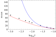
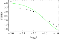
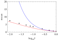
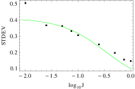
Numerically, we consider an ensemble of paths described by (64). The relaxation time is then defined as such when the p-value of the ensemble of $X$ conforming to the IGa distribution is larger than 0.1. In our computation, 5000 paths are considered for each relaxation time. Our results are shown in Fig. 24. Clearly, our estimates (67) - (69) with $c_{1}=1$ and $c_{2}=1/4$ fit the data quite well.

Figure 24: Relaxation times of an inverse gamma process. Top: $\sigma=\sqrt{0.1}$ and bottom: $\sigma=1$. Mean: black squares: numerical results; red line: theoretical estimate (67) with $c_{1}=1$; blue line: theoretical estimate (68). STDEV: black squares: numerical results; green line: theoretical estimate (69) with $c_{2}=1/4$

Appendix G Maximum likelihood estimation of GGa and GIGa

For PDF $f(x|\theta)$, with parameter(s) $\theta$ and a dataset $\{x_{i}\}$ of size $n$, the likelihood function is

$$\prod_{i=1}^{n}f(x_{i}|\theta)$$ (70)

and the log-likelihood function is

$$\frac{1}{n}\sum_{i=1}^{n}\log f(x_{i}|\theta).$$ (71)

The maximum likelihood estimation of $\theta$ should maximize the log-likelihood function. Here we consider the case of GGa and GIGa. Generalized Student’s t-distribution is discussed in MaThesis2013 .

Since, as already mentioned, the PDFs of GGa and GIGa formally follow $\text{GGa}(x;\alpha,\beta,\gamma)\xleftrightarrow{\gamma\leftrightarrow-\gamma}-\text{GGa}(x;\alpha,\beta,-\gamma)=-\text{GIGa}(x;\alpha,\beta,\gamma)$, it is sufficient to consider GGa. Setting to zero partial derivatives over $\alpha$, $\beta$, and $\gamma$ of the log-likelihood function for $\text{GGa}(x;\alpha,\beta,\gamma)$ gives

$$(\frac{1}{n}\sum_{i=1}^{n}\log x_{i}^{\gamma})-\log\beta^{\gamma}-\psi(\alpha)=0$$ (72)

$$\frac{\frac{1}{n}\sum_{i=1}^{n}x_{i}^{\gamma}}{\beta^{\gamma}}-\alpha=0$$ (73)

$$1-\frac{1}{n}\sum_{i=1}^{n}\left(\frac{x_{i}^{\gamma}}{\beta^{\gamma}}-\alpha\right)\log\frac{x_{i}^{\gamma}}{\beta^{\gamma}}=0.$$ (74)

With the definition

$$\frac{1}{n}\sum_{i=1}^{n}f(x_{i})=\overline{f(x)},$$ (75)

we obtain

$$\overline{\log x^{\gamma}}-\log\beta^{\gamma}-\psi(\alpha)=0$$ (76)

$$\frac{\overline{x^{\gamma}}}{\beta^{\gamma}}-\alpha=0$$ (77)

$$1-\overline{\left(\frac{x^{\gamma}}{\beta^{\gamma}}-\alpha\right)\log\frac{x^{\gamma}}{\beta^{\gamma}}}=0.$$ (78)

Substitution of Eq. (77) into (76) and Eq. (78) yileds

$$\overline{\log x^{\gamma}}-\log\overline{x^{\gamma}}+\log\alpha-\psi(\alpha)=0$$ (79)

and

$$\alpha=\left[{\overline{\left(\frac{x^{\gamma}\log x^{\gamma}}{\overline{x^{\gamma}}}-\log x^{\gamma}\right)}}\right]^{-1}.$$ (80)

Eqs. (79) and (80) form the basis of a maximum likelihood estimation program. Given a $\gamma$, from (80), we calculate $\alpha$ and then insert $\alpha$ into the lhs of (79). A bisection method can be realized over $\gamma$. For more details, see MaThesis2013 . We note that Eqs. (79) and (80) result in either GGa ($\gamma>0$), or GIGa ($\gamma<0$). MaThesis2013 .

Appendix H Log-log plot of distribution tails

The exponent of a power law tail can be easily calculated once we notice that

$$1-\text{CDF}(x)=\int_{x}^{+\infty}\text{PDF}(x)dx.$$ (81)

If $\text{PDF}(x)\propto x^{-1-k}$ with $x\gg 1$, then

$$\log(1-\text{CDF}(x))\propto\text{const}-k\log x.$$ (82)

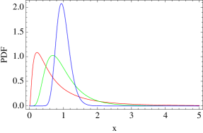
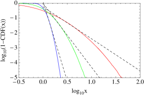
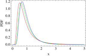
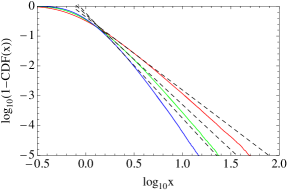
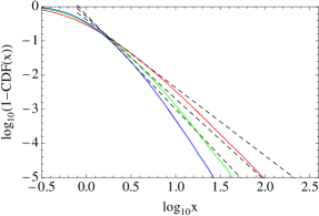
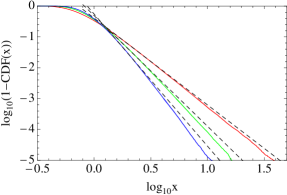
In Figs. 26 and 26, we show the log-log plot of the tail of LN and IGa distributions respectively. Clearly, a straight line fit is considerably better for the latter, even though the fitted slope does not agree with the theoretical value. Towards this end, in Fig. 27, we show log-log plots of the tail of GIGa distributions for $\gamma=0.5$ and $\gamma=2$. The empirical trend emerging form the IGa and GIGa plots is that the straight line fits of log-log plots become progressively better as $\gamma$ gets larger.

Figure 25: Top: plots of PDF of $\text{LN}(x;\mu,\sigma)$ with mean 1. The left red, middle green, and right blue curves correspond to parameter $\sigma=1,0.5$, and $0.2$ respectively. Bottom: log-log plots of simulated data sampled from the LN distributions. Below $-1$ of the y-axis, the left blue, middle green, and right red curves correspond to $\sigma=0.2,0.5$, and $1$ respectively. The dashed lines are fitting of $\log_{10}(1-\text{CDF}(x))$ vs. $\log_{10}x$ in a range of CDF from 0.9 to 0.99.

Figure 26: Top: plots of PDF of $\text{IGa}(x;\alpha,\beta)$ with mean 1. The left red, middle green, and right blue curves correspond to $\alpha=3,4$, and $5$ respectively. Bottom: log-log plots of simulated data sampled from the IGa distributions. Below $-1$ of the y-axis, the left blue, middle green, and right red curves correspond to $\alpha=5,4$, and $3$ respectively. The dashed lines with slopes $-3.5,-3.0$, and $-2.5$ respectively are fitting of $\log_{10}(1-\text{CDF}(x))$ vs. $\log_{10}x$ in a range of CDF from 0.9 to 0.99.

Figure 27: Log-log plots of simulated data sampled from GIGa distributions $\text{GIGa}(x;\alpha,\beta,0.5)(top)$ and $\text{GIGa}(x;\alpha,\beta,2)$ (bottom) with mean 1. Below $-1$ of the y-axis, the left blue, middle green, and right red curves correspond to $\alpha=2.5,2$, and $1.5$ respectively. The dashed lines with slopes $-2.8,-2.4$, and $-2.0$ respectively (top) and $-4.3,-3.6$, and $-2.8$ (bottom) are fitting of $\log_{10}(1-\text{CDF}(x))$ vs. $\log_{10}x$ in a range of CDF from 0.9 to 0.99.

To understand this $\gamma$-dependence the difference between the theoretical and fitted slope, we consider the local slope of the log-log plot.

$$\frac{d\log(1-\text{CDF}(x))}{d\log x}.$$ (83)

For GIGa (and IGa, $\gamma=1$), the local slope is given by

$$\frac{\gamma e^{-\left(\frac{\beta}{x}\right)^{\gamma}}\left(\frac{\beta}{x}\right)^{\alpha\gamma}}{\Gamma(\alpha)\left(Q\left(\alpha,\left(\frac{\beta}{x}\right)^{\gamma}\right)-1\right)}$$ (84)

with the regularized gamma function $Q(s,x)={\Gamma(s,x)}/{\Gamma(s)}$, where $\Gamma(s,x)\equiv\int_{x}^{\infty}t^{s-1}e^{-t}dt$ is the incomplete gamma function. The local slopes are shown, as function of $x$ in Figs. 28 and 29 respectively. It is clear that the local slope can differ substantially from its limiting (saturation) value. As $\gamma$ becomes larger, the local slope tends closer to its limiting value.

Figure 28: Local slope of log-log plot of IGa distribution IGa$(x;\alpha,\beta)$ with mean 1 ($\beta=\Gamma(\alpha)/\Gamma(\alpha-1)$). The left column is the log-log plot and the right one is the local slope of the log-log plot from Eq. (84). $\alpha$ is 2, 3, 5, and 7 for the first, second, third, and fourth rows respectively. The red lines are $-\alpha$: the limit of the local slope when $x\rightarrow\infty$.

Figure 29: Local slope of log-log plot of GIGa$(x;\alpha,\beta,\gamma)$ with mean 1 ($\beta=\Gamma(\alpha)/\Gamma(\alpha-1/\gamma)$). The left column is the log-log plot and the right one is the local slope of the log-log plot from Eq. (84). $\{\alpha,\gamma\}$ is $\{6,0.5\}$, $\{10,0.5\}$, $\{1.5,2\}$, and $\{2.5,2\}$ for the first, second, third, and fourth rows respectively. The red lines are $-\alpha\gamma$: the limit of the local slope when $x\rightarrow\infty$.

For the LN distribution, the local slope is given by

$$\frac{\sqrt{\frac{2}{\pi}}e^{-\frac{(\log x-\mu)^{2}}{2\sigma^{2}}}}{\sigma\left(1+\text{erf}\left(-\frac{\log x-\mu}{\sqrt{2}\sigma}\right)\right)},$$ (85)

which slowly decreases with $x$. But as is clear from (85) and Fig. 30, the local slope does not saturate when $x\rightarrow\infty$.

Figure 30: Local slope of log-log plot of lognormal distribution. The mean of the distribution is set as 1 through $\mu=-\sigma^{2}/2$. The left column is the log-log plot and the right one is the local slope of the log-log plot in Eq. (85). $\sigma$ is 0.2, 0.5, 1, and 2 for the first, second, third, and fourth row respectively. The jagged part of the top right plot is due to computational precision.

References

• (1) T. Ma, J. G. Holden, and R. A. Serota, Physica A: Statistical Mechanics and its Applications 392, 2434 (2013).
• (2) D. West and B. West, Int. J. Mod. Phys. B 26, 1230010 (2012).
• (3) T. Ma, J. G. Holden, and R. A. Serota, In preparation (2013).
• (4) J. Hull, Options, Futures, and Other Derivatives, 3rd ed (Prentice Hall, Upper Saddle River, NJ, 1997).
• (5) J. Gatheral, The Volatility Surface: a Practitioner’s Guide (Wiley & Sons, Hoboken, New Jersey, 2006).
• (6) P. D. Praetz, Journal of Business 45, 49 (1972).
• (7) E. Platen and R. Rendek, Journal of Statistical Theory and Practice 2, 233 (2008).
• (8) A. Gerig, J. Vicente, and M. A. Fuentes, Phys. Rev. E 80, 065102 (2009).
• (9) D. B. Nelson, Journal of Econometrics 45, 7 (1990).
• (10) J.-C. Duan, Mathematical Finance 5, 13 (1995) (GARCH(1,1)11(1,1) model is used in the theory of option pricing).
• (11) J. B. Wiggins, Journal of Financial Economics 19, 351 (1987).
• (12) VIX Historical Price Data, http://www.cboe.com/micro/vix/historical.aspx.
• (13) Volatility Indexes, http://www.cboe.com/micro/volatility/introduction.aspx.
• (14) VXO, http://www.cboe.com/micro/vxo/.
• (15) Standard & Poor’s, http://www.standardandpoors.com/.
• (16) Yahoo! Finance, http://finance.yahoo.com/.
• (17) Economic Research Federal Reserve Bank of St. Louis: S&P 500 Stock Price Index (SP500), http://research.stlouisfed.org/fred2/series/SP500/downloaddata?cid=32255.
• (18) Economic Research Federal Reserve Bank of St. Louis: Dow Jones Industrial Average (DJIA), https://research.stlouisfed.org/fred2/series/DJIA/downloaddata?cid=32255/.
• (19) T. Ma, Ph.D. thesis, University of Cincinnati (2013).
• (20) J.-P. Bouchaud and M. Mézard, Physica A: Statistical Mechanics and its Applications 282, 536 (2000).
• (21) S. L. Heston, The Review of Financial Studies 6, 327 (1993).
• (22) M. H. Stanley, L. A. Amaral, S. V. Buldyrev, S. Havlin, H. Leschhorn, P. Maass, M. A. Salinger, and H. E. Stanley, Nature 379, 804 (1996).
• (23) P. Cizeau, Y. Liu, M. Meyer, C.-K. Peng, and H. E. Stanley, Physica A: Statistical Mechanics and its Applications 245, 441 (1997).
• (24) Y. Liu, P. Gopikrishnan, Cizeau, Meyer, Peng, and H. E. Stanley, Phys. Rev. E 60, 1390 (1999).
• (25) P. Gopikrishnan, V. Plerou, L. A. N. Amaral, M. Meyer, and H. E. Stanley, Phys. Rev. E 60, 5305 (1999).
• (26) V. Plerou, P. Gopikrishnan, L. A. N. Amaral, M. Meyer, and H. E. Stanley, Phys. Rev. E 60, 6519 (1999).
• (27) The Generalized Gamma Distribution and Reliability Analysis, http://www.weibull.com/hotwire/issue15/hottopics15.htm.
• (28) J. Lawless, Statistical Models and Methods for Lifetime Data, (Wiley & Sons, New York, 1982).
• (29) L. O. Scott, Journal of Financial and Quantitative Analysis 22, 419 (1987).
• (30) S. Jackman, Bayesian Analysis for the Social Sciences (Wiley & Sons, 2009).