AVERAGE STRETCH FACTOR: HOW LOW DOES IT GO?

In a geometric graph, $G$, the stretch factor between two vertices, $u$ and $w$, is the ratio between the Euclidean length of the shortest path from $u$ to $w$ in $G$ and the Euclidean distance between $u$ and $w$. The average stretch factor of $G$ is the average stretch factor taken over all pairs of vertices in $G$. We show that, for any constant dimension, $d$, and any set, $V$, of $n$ points in $\mathbb{R}^{d}$, there exists a geometric graph with vertex set $V$, that has $O(n)$ edges, and that has average stretch factor $1+o_{n}(1)$. More precisely, the average stretch factor of this graph is $1+O((\log n/n)^{1/(2d+1)})$. We complement this upper-bound with a lower bound: There exist $n$-point sets in $\mathbb{R}^{2}$ for which any graph with $O(n)$ edges has average stretch factor $1+\Omega(1/\sqrt{n})$. Bounds of this type are not possible for the more commonly studied worst-case stretch factor. In particular, there exists point sets, $V$, such that any graph with worst-case stretch factor $1+o_{n}(1)$ has a superlinear number of edges.

1 Introduction

A geometric graph is a simple undirected graph whose vertex set is a set of points in $\mathbb{R}^{d}$. The average stretch factor of a finite connected geometric graph, $G=(V,E)$, with vertex set $V\subset\mathbb{R}^{d}$ and edge set $E$ is

$$\operatorname{asf}(G)=\binom{n}{2}^{-1}\sum_{\{u,w\}\in\binom{V}{2}}\frac{\|uw\|_{G}}{\|uw\|}$$ (1)

where $\|uw\|$ denotes the Euclidean distance between $u$ and $w$ and $\|uw\|_{G}$ denotes the cost of the shortest path from $u$ to $w$ in the graph $G$, where each edge of $G$ is weighted by the Euclidean distance between its endpoints. (Here, and forever, $n=|V|$.)

The related notion of worst-case stretch factor, defined as

$$\operatorname{sf}(G)=\max_{\{u,w\}\in\binom{V}{2}}\frac{\|uw\|_{G}}{\|uw\|}\enspace,$$

has been studied extensively. A graph, $G$, with $\operatorname{sf}(G)\leq t$ is called a $t$-spanner. The construction of and applications of $t$-spanners is the subject of intensive research and there is a book [16] and handbook chapter [13] devoted to the topic.

The average or worst-case stretch factor of the complete graph with vertex set $V\subset\mathbb{R}^{d}$ is 1 and, if $V$ contains no collinear triples, then any graph on $V$ with fewer than $\binom{n}{2}$ edges will have (average and worst-case) stretch factor strictly greater than 1. At the other extreme, any connected graph with vertex set $V$ has at least $n-1$ edges. Thus, there seems to be a tradeoff between the following two requirements on a graph $G=(V,E)$ that is constructed from a given point set, $V$:

1. $G$ should be as sparse as possible, ideally $|E|\in O(n)$; and

2. $G$ should have small (average or worst-case) stretch factor, ideally $\operatorname{(a)sf}(G)=1+o_{n}(1)$.

In this paper we are interested in determining to what extent we can simultaneously satisfy these two conflicting goals.

For worst-case stretch factor, it is not possible to achieve the preceding two goals simultaneously: Elkin and Solomon [11] show that there exists point sets $V\subset\mathbb{R}^{d}$ such that any graph $G=(V,E)$ having $\operatorname{sf}(G)\leq 1+\varepsilon$ has maximum degree $\Omega(1/\varepsilon^{d-1})$. A variant of their argument shows that, for some point sets, a constant fraction of vertices must have degree $\Omega(1/\varepsilon^{d-1})$ and therefore the graph must have $\Omega(n/\varepsilon^{d-1})$ edges [19]. In short: achieving a worst-case stretch factor of $1+o_{n}(1)$ requires $\omega(n)$ edges.

1.1 New Results and Outline

In this paper we show that, for average stretch factor, it is possible to simultaneously achieve both desired properties: For any constant dimension, $d$, and any set $V\subset\mathbb{R}^{d}$, there exists a geometric graph $G=(V,E)$ having $|E|\in O(n)$ edges and such that $\operatorname{asf}(G)=1+o_{n}(1)$. More precisely,

$$\operatorname{asf}(G)=1+O((\log n/n)^{1/(2d+1)})\enspace.$$

The proof of this result is in Section 2 and constitutes the bulk of the paper.

In Section 3, we show that graphs with small average stretch factor can be constructed efficiently. In particular, we present an $O(n\log n)$ time Monte-Carlo algorithm that, with high probability, constructs a graph with average stretch factor $1+o_{n}(1)$. In Section 4 we present a simple lower-bound that shows our upper-bound is at least of the right flavour: For every positive integer $n$, there exists an $n$ point set in $\mathbb{R}^{2}$ on which any graph with $O(n)$ edges has average stretch factor $1+\Omega(1/\sqrt{n})$. In Section 5 we relate the parts of our construction to some real-world networks and discuss directions for future work.

1.2 Relation to Previous Work

In the more general context of embedding metric spaces into ultrametrics, Abraham et al. [1, 2] show that for any point set, $V$, there exists a spanning tree, $T=(V,E)$, with $\operatorname{asf}(T)\in O(1)$. Thus, it is always possible to construct a very sparse graph with constant average stretch factor. This contrasts sharply with worst-case stretch factor: Any spanning tree on the vertices of a regular $n$-gon has worst-case stretch factor $\Omega(n)$ [12, Lemma 15].

Aldous and Kendall [3, Section 5.3] show that, for any well-distributed point set $V\subset[0,\sqrt{n}]^{2}$ and any $\varepsilon>0$ there exists a Steiner network, $N=(V^{\prime},E)$, with $V^{\prime}\supseteq V$, of total edge length $\sum_{uw\in E}\|uw\|\leq(1+\varepsilon)\operatorname{msst}(V)$ and for which,

$$\binom{n}{2}^{-1}\sum_{\{u,w\}\in\binom{V}{2}}\frac{\|uw\|_{N}}{\|uw\|}=1+O((\log n/n)^{1/3}).$$

Here $\operatorname{msst}(V)$ denotes the length of the minimum Steiner spanning tree of the points in $V$. Thus $N$ is a graph that is only slightly longer than the minimum length connected graph that contains $V$ and the average stretch factor of $N$ (taken over pairs in $V$) tends to 1. In this construction, we call the points in $V^{\prime}\setminus V$ Steiner points.

In the work of Aldous and Kendall, which was the starting point for the current work, the authors focus on finding a light network; one whose total edge length is small. In the current paper, we focus instead on finding a sparse network; one with a small number of edges. With this shift of focus in mind, Aldous and Kendall’s work immediately raises three questions: (1) Can a similar result be proven without making any form of “well-distributed” assumption on the points in $V$? (2) Can a similar result be proven without using Steiner points? (3) Can a similar result be proven for point sets in $\mathbb{R}^{d}$? Our results answer all three of these questions in the affirmative.

We note that it does not seem easy to answer any of the preceding questions using a modification of Aldous and Kendall’s construction. (1) Their proof uses the well-distributed assumption to argue that most pairs of points are at distance at least $n^{\gamma}$, for any $\gamma<1/2$ [3, Section 5.3]. (2) their construction consists of a minimum Steiner spanning tree of $V$, some additional random line segments, and some additional segments that form a grid. Anywhere two segments cross, a vertex is added to $V^{\prime}$, so this construction makes essential use of Steiner points. (3) The main technical tool used in their proof is a new result on the lengths of boundaries of certain cells in arrangements of random lines [3, Theorems 3 and 4]. In dimensions greater than 2, arrangements of lines do not decompose space into cells, so it seems difficult to generalize this result to higher dimensions.

2 The Construction

Our construction of a good average stretch factor graph, $G=(V,E)$, makes use of a clustering of the points of $V$ into $O(n/k)$ clusters, each of size at most $k$, that we call a $k$-partition. In the next subsection, we define $k$-partitions and show how to compute them. In the subsequent subsection we show how to construct the graph $G$.

2.1 $k$-Partitions

We make use of the following construct: A $k$-partition of a set $V$ of $n$ points in $\mathbb{R}^{d}$ consists of a set, $D$, of balls and an assignment $f:V\to D$ such that

1. $|D|\in O(n/k)$;

2. for each $u\in V$, $u\in f(u)$ (i.e., $u$ is assigned to a ball that contains $u$);

3. for each $\Delta\in D$, $|\{u\in V:f(u)=\Delta\}|\leq k$ (i.e., at most $k$ points are assigned to each ball);

4. for every $r>0$ and $p\in\mathbb{R}^{d}$, the number of balls in $D$ whose radius is in the range $[r,2r)$ and that contain $p$ is $O(1)$; and

5. for every $r\geq 0$ and every ball, $B$, of radius $r$,

   $$|\{u\in V:u\in B\text{ and }\operatorname{radius}(f(u))\geq r\}|\in O(k)$$

   (i.e., there are only $O(k)$ points of $V$ that are in $B$ and that are assigned to balls of radius at least $r$).

Note that, aside from Properties 4 and 5, there is very little structure to the balls in $D$. In particular, balls in $D$ may overlap and may even contain each other.

Lemma 1.

For any constant dimension, $d$, and any set $V$ of $n$ points in $\mathbb{R}^{d}$, a $k$-partition of $V$ exists and can be computed in $O(n\log n)$ time.

Proof.

We construct a $k$-partition using the binary fair-split tree, $T=T(V)$, which is defined recursively as follows [9]: If $V$ consists of a single point, $u$, then $T$ contains a single node corresponding to $u$. Otherwise, consider the minimal axis-aligned bounding box, $B(V)$, that contains $V$. The root of $T$ corresponds to $B(V)$ and this box is split into two boxes $B_{1}(V)$ and $B_{2}(V)$ by cutting $B(V)$ with a hyperplane in the middle of its longest side. The left and right subtrees of the root are defined recursively by constructing fair-split trees for $B_{1}(V)\cap V$ and $B_{2}(V)\cap V$. See Figure 1.

Figure 1: A fair-split tree for $V$ repeatedly splits the bounding box $B(V)$ in the middle of its longest side.

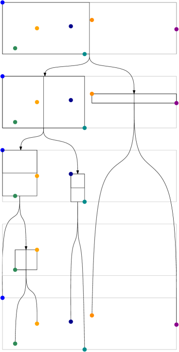
The $k$-Partition.

For each node, $u$, of $T$ there is a naturally defined subset $V(u)\subseteq V$ of points associated with $u$ as well as a bounding box $B(u)=B(V(u))$. Since $T$ is a binary tree with $2n-1$ nodes, it has a set of $t-1$ edges whose removal partitions the vertices of $T$ into $t\in O(n/k)$ maximally-connected components $C_{1},\ldots,C_{t}$, each having at most $k$ vertices.

For each $i\in\{1,\ldots,t\}$, let $u_{i}$ denote the node in $C_{i}$ of minimum depth, and call $u_{i}$, the root of $C_{i}$. To obtain the balls, $\Delta_{1},\ldots,\Delta_{t}$, of the $k$-partition we take, for each $i\in\{1,\ldots,t\}$ the smallest ball, $\Delta_{i}$ that contains $B(u_{i})$. For the mapping $f$, we map the point associated with each leaf, $w$, of $T$ to the unique ball $\Delta_{i}$, where $C_{i}$ contains $w$. See Figure 2.

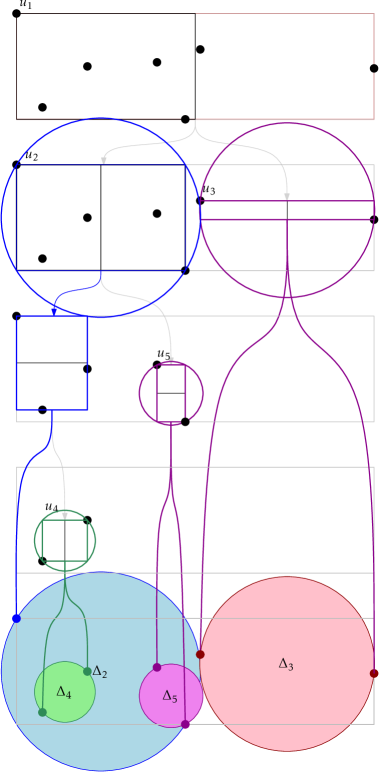
Figure 2: The fair-split tree is partitioned into subtrees of size $k$ (${}=3$) by removing $O(n/k)$ edges. The root, $u_{i}$, of each subtree defines a ball, $\Delta_{i}$, in the $k$-partition. (The ball $\Delta_{1}$ is omitted from this figure.)

The fair-split tree, $T$, and the boxes, $B(u)$, associated with each node, $u$, of $T$ can be computed in $O(n\log n)$ time [9]. The partition of the vertices of $T$ into components $C_{1},\ldots,C_{t}$ can easily be done in $O(n\log n)$ time by repeatedly finding an edge of a component of size $k^{\prime}>k$ whose removal partitions that component into two pieces each of size at most $\lceil 2k^{\prime}/3\rceil$. Thus, the construction of $D$ and $f$ can be accomplished in $O(n\log n)$ time.

The set of balls $D=\{\Delta_{1},\ldots,\Delta_{t}\}$ and the mapping $f:V\to D$ described in the preceding paragraphs clearly satisfy Properties 1–3 in the definition of a $k$-partition. What remains is to show that they also satisfy Properties 4 and 5.

For a node $u$ in $T$, with $B(u)=[a_{1},b_{1}]\times\cdots\times[a_{d},b_{d}]$, define $L_{i}(u)=b_{i}-a_{i}$ and let $L(u)=\max\{L_{i}(i):i\in\{1,\ldots,d\}\}$ denote the length of $B(u)$’s longest side. To establish Properties 4 and 5, we make use of the following result on fair-split trees [16, Lemma 9.4.3]:

Lemma 2.

Let $C$ be a box whose longest side has length $\ell$ and let $\alpha>0$ be any positive real number. Let $w_{1},\ldots,w_{s}$ be some nodes of a fair-split tree, $T$, such that

1. the sets $V(w_{i})$ are pairwise disjoint, for all $i\in\{1,\ldots,s\}$;

2. $L(w_{i})\geq\ell/\alpha$, for all $i\in\{1,\ldots,s\}$; and

3. $B(w_{i})$ intersects $C$, for all $i\in\{1,\ldots,s\}$.

Then $s\leq(2\alpha+2)^{d}$.

Property 4.

To prove that the balls in $D$ satisfy Property 4, let $\{\Delta_{i_{1}},\ldots,\Delta_{i_{q}}\}\subseteq D$ be the subset of balls in $D$ having radii in the interval $[r,2r)$ and that all contain some common point, $p\in\mathbb{R}^{d}$. Then each such ball, $\Delta_{i_{j}}$ corresponds to a node $u_{i_{j}}$ of $T$ such that

$$\frac{2r}{\sqrt{d}}\leq L(u_{i_{j}})\leq 4r\enspace.$$ (2)

Each box, $B(u_{i_{j}})$, intersects the ball of radius $2r$ centered at $p$. (Indeed, the center of $B(u_{i_{j}})$ is contained in this ball.) Therefore, each box $B(u_{i_{j}})$ intersects the box, $C$, of side-length $4r$ centered at $p$.

We are almost ready to apply Lemma 2 to $C$—whose side length is $\ell=4r$—and the vertex set $w_{1},\ldots,w_{q}=u_{i_{1}},\ldots,u_{i_{q}}$. For each $j\in\{1,\ldots,q\}$, $B(u_{i_{j}})$ intersects $C$, so Condition 3 of Lemma 2 is satisfied. Furthermore, (2) states that $L(u_{i_{j}})\geq 2r/\sqrt{d}=\ell/(2\sqrt{d})$, so Condition 2 of Lemma 2 is satisfied with $\alpha=2\sqrt{d}$. Unfortunately, there is still a little more work to do since the nodes $u_{i_{1}},\ldots,u_{i_{t}}$ do not necessarily satisfy Condition 1 of Lemma 2.

To proceed, we partition $u_{i_{1}},\ldots,u_{i_{q}}$ into a small number of subsets, each of which satisfies Condition 1 of Lemma 2. Observe that Condition 1 of Lemma 2 is equivalent to the statement that no $w_{i}$ is an ancestor of $w_{j}$ for any $\{i,j\}\subseteq\{1,\ldots,s\}$. A key observation is that, if $u$ is an ancestor of $w$ in a fair-split tree, $T$, and the difference in depth between $u$ and $w$ is at least $d$, then

$$L(u)\geq 2L(w)\enspace.$$

This, and (2), implies that, if $u_{i_{j}}$ is an ancestor of $u_{i_{j^{\prime}}}$ then

$$\operatorname{depth}(u_{i_{j^{\prime}}})-\operatorname{depth}(u_{i_{j}})\leq d\log(2\sqrt{d})\enspace.$$

Thus, we can partition $u_{i_{1}},\ldots,u_{i_{q}}$ into $z=\lceil d\log(2\sqrt{d})\rceil$ subsets, $S_{0},\ldots,S_{z-1}$, each of which satisfies Condition 1 of Lemma 2, by assigning $u_{i_{j}}$ to the subset $S_{\operatorname{depth}(u_{i_{j}})\bmod z}$.

Now, Lemma 2 implies that, for each $i\in\{0,\ldots,z-1\}$,

$$|S_{i}|\leq(4\sqrt{d}+2)^{d}$$

so that

$$q=\sum_{i=0}^{z-1}|S_{i}|\leq(4\sqrt{d}+2)^{d}z=(4\sqrt{d}+2)^{d}\lceil d\log(2\sqrt{d})\rceil\in O(1)\enspace.$$

Thus, for any point $p\in\mathbb{R}^{d}$, the set of balls in $D$ whose radius is in the interval $[r,2r)$ and that contain $p$ has size $O(1)$. Therefore the balls in $D=\{\Delta_{1},\ldots,\Delta_{t}\}$ satisfy Property 4 in the definition of a $k$-partition.

Property 5.

To study Property 5, it is easier to work with the bounding boxes, $B(u)$, associated with each node, $u$, in the fair-split tree as well as the box, $C$, of side length $2r$ that contains the ball $B$. See Figure 3. Observe that if some ball, $\Delta_{i}$, is assigned a point in $B$, then the box $B(u_{i})$ intersects $C$. Thus, we need only consider the set $U\subseteq\{u_{1},\ldots,u_{t}\}$ that contains only those nodes $u_{i}$ such that $\operatorname{radius}(\Delta_{i})\geq r$ and $B(u_{i})$ intersects $C$.

Figure 3: Proving Property 5 of $k$-partitions.

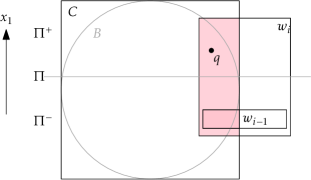
For each $u\in U$, (2) implies that $L(u)\geq 2r/\sqrt{d}$. Therefore, by Lemma 2, $U$ contains a subset, $U^{\prime}$, of size at most $(4\sqrt{d}+2)^{d}\in O(1)$ such that every node in $U$ is an ancestor of some node in $U^{\prime}$. Thus, the elements of $U$ can be covered by $O(1)$ paths, each of which goes from a node in $U^{\prime}$ to the root of $T$. It suffices to consider the contribution of one such path, $w_{1},\ldots,w_{\ell}$, where $w_{1}\in U^{\prime}$ and $w_{\ell}$ is the root of $T$.

For each $i\in\{1,\ldots,\ell\}$, let $C_{i}$, denote the box $C\cap B(w_{i})$. Since $B(w_{1})\subset\cdots\subset B(w_{\ell})$, we have that $C_{1}\subseteq\cdots\subseteq C_{\ell}$. Observe that, for each $w_{i}$, the ball associated with $w_{i}$ is not assigned any points in $B(w_{i-1})$. Thus, it is sufficient to show that there are $O(1)$ values of $i$ for which $V\cap C_{i}\neq V\cap C_{i-1}$; for each such $i$, the number of elements assigned to the corresponding ball of the $k$-partition is at most $k$.

We extend the side-length notation, $L_{i}$, to any box, $B=[a_{1},b_{1}]\times\cdots[a_{d},b_{d}]$, so that $L_{i}(B)=|b_{i}-a_{i}|$ and define the total side length $\sum_{i=1}^{d}L_{i}(B)$. We will show that, for each $i\in\{2,\ldots,\ell\}$, at least one of the following statements is true

1. $V\cap C_{i}=V\cap C_{i-1}$;

2. the total side length of $C_{i}$ exceeds that of $C_{i-1}$ by at least $L(w_{1})/2$; or

3. $C_{i}$ intersects a side of $C$ that is not intersected by $C_{i-1}$.

This is sufficient to prove the result since Case 1 does not result in any new points included in $B$, Case 2 can occur at most $4rd/L(w_{1})\in O(1)$ times, and Case 3 can occur at most $2d\in O(1)$ times.

To see why one of the preceding cases must occur, suppose that neither Case 1 nor Case 3 applies. Since Case 1 does not apply, there is some point $q\in V\cap C_{i}$ that is not in $C_{i-1}$. Without loss of generality, assume that the fair-split tree cuts $B(w_{i})$ with a plane, $\Pi$, that is perpendicular to the $x_{1}$-axis. Let $\Pi^{+}$ and $\Pi^{-}$ denote the closed halfspaces bounded by $\Pi$ that contain $q$ and $B(w_{i-1})$, respectively. Then we have that

$$L_{1}(B(w_{i})\cap\Pi^{+})=L_{1}(w_{i})/2\geq L(w_{i-1})/2\geq L(w_{1})/2\enspace.$$

Observe that $B(w_{i})$ does not intersect the side of $C$ that is parallel to $\Pi$ and contained in $\Pi^{+}$ (since, otherwise, Case 3 would apply). This implies that

$$L_{1}(C_{i})\geq L_{1}(C_{i-1})+L(w_{1})/2\enspace.$$

Thus, if neither Case 1 nor Case 3 applies to $u_{i}$, then Case 2 applies. This completes the proof. ∎

2.2 The Graph $G$

With the availability of $k$-partitions, we are now ready to construct a graph $G$ with low average stretch factor. In the following construction, positive valued variables $c,k\in\omega_{n}(1)$ and $\epsilon\in o_{n}(1)$ are used without being specified. Values of these variables that optimize the average stretch factor of $G$ will be given in the proof of Theorem 1. In the meantime, the reader can mentally assign the values $c=k=\log n$ and $\epsilon=1/\log n$, which are sufficient to prove that $\operatorname{asf}(G)=1+o_{n}(1)$.

Hubs.

We begin with a $k$-partition $(\{\Delta_{1},\ldots,\Delta_{n^{\prime}}\},f)$ of $V$. For each $i\in\{1,\ldots,n^{\prime}\}$, let $r_{i}$ denote the radius of $\Delta_{i}$. We will use the convention that $\Delta_{1},\ldots,\Delta_{n^{\prime}}$ are ordered by increasing radii, so that $r_{i}\leq r_{j}$ for each $1\leq i<j\leq n^{\prime}$. For each $i\in\{1,\ldots,n^{\prime}\}$, let $V_{i}=\{u\in V:f(u)=\Delta_{i}\}$; that is, $V_{i}$ is the set of points assigned to the ball $\Delta_{i}$. For each set $V_{i}$, we choose a hub, $u_{i}\in V_{i}$, arbitrarily. Let $H=\{u_{1},\ldots,u_{n^{\prime}}\}$ denote the set of hubs and recall that $|H|=n^{\prime}\in O(n/k)$.

Figure 4: $G$ contains a 2-spanner of $V$ (gray edges) as well as $O(n/k)$ hubs whose centers are interconnected by a $(1+1/k^{1/(d-1)})$-spanner (red edges)

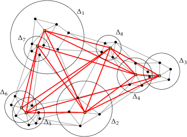
Roads and Highways.

Our graph $G$ starts with two spanner constructions. The first spanner (the roads), denoted by $G_{2}=(V,E_{2})$, is a 2-spanner of $V$, and has $O(n)$ edges [8, 18, 20]. The next spanner (the highways), denoted by $G_{1}=(H,E_{1})$, is a $(1+1/k^{1/(d-1)})$-spanner of $H$, and has $O(k|H|)=O(n)$ edges [10, 17].

With $G_{1}$ and $G_{2}$ we have, for any $u,w\in V$:

$$\frac{\|uw\|_{G}}{\|uw\|}\leq\begin{cases}1+1/k^{1/(d-1)}&\text{if $u,w\in H$ (by using $G_{1}$)}\\ 2&\text{in any case (by using $G_{2}$).}\end{cases}$$

Covering a Nearby Cluster.

Informally, the idea behind the graphs $G_{1}$ and $G_{2}$ is that, if $u\in V_{i}$ and $w\in V_{j}$ are “far apart” (relative to $r_{i}$ and $r_{j}$), then the path from $u$ to $w$ that goes from $u$ to $u_{i}$ via roads ($G_{2}$), then to $u_{j}$ via highways ($G_{1}$), and then onto $w$ via roads again should have length $(1+o_{n}(1))\|uw\|$. Of course, this only works if $u$ and $w$ are far apart. The final step of our construction attempts to deal with the majority of cases where $u$ and $w$ are not far apart.

To make the preceding ideas precise, let $D_{i}$ be the ball centered at the center of $\Delta_{i}$ and having radius $cr_{i}$. Points of $V$ that are in $D_{i}$ can be problematic for $V_{i}$; there is no guarantee that such points have paths with $1+o_{n}(1)$ stretch factor to the points in $V_{i}$.

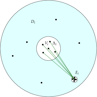
For each $i\in\{1,\ldots,n^{\prime}\}$, we find a ball, $E_{i}$, of radius $r_{i}/c$, that intersects $D_{i}$, and that contains the maximum number of points of $V$. (Note that this may include points of $V$ in $V_{i}$ or outside of $D_{i}$.) We then add edges joining each of the points in $V_{i}$ to a carefully chosen point $w_{i}\in E_{i}$. See Figure 5.

The point $w_{i}$ is chosen as follows: For each point $w\in V$, let $i(w)\in\{1,\ldots,n^{\prime}\}$ denote the smallest index such that $w\in E_{i(w)}$ and $|E_{i(w)}\cap V|\geq\epsilon n$; if no such index exists, let $i(w)=\infty$. The point $w_{i}\in E_{i}$ is selected to be any of the points in $E_{i}$ that minimizes $i(w)$. This concludes the description of the graph $G$.

Figure 5: The ball $E_{i}$ captures as many points of $V$ as possible while still intersecting $D_{i}$.

2.3 Two Illustrative Examples

Before delving into the proof that $G$ has low average stretch factor, it may be helpful to study two examples that illustrate why the balls $E_{1},\ldots,E_{n^{\prime}}$ are needed and why the choice of the representative vertices, $w_{i}\in E_{i}$, is important.

Example 1: Exponential Grids.

The first example is a set of points arranged as a sequence of $\sqrt{k}\times\sqrt{k}$ grids, $G_{0},\ldots,G_{n/k-1}$. The grid $G_{i}$ has its center on the x-axis at x-coordinate $2^{i+1}-1$, and has side length $2^{i}$ (see Figure 6). The natural $k$-partition of this grid is the one that assigns all points in each $G_{i}$ to a single ball, $\Delta_{i}$. In this grid, if we consider $G_{i}$, for some large value of $i$, we see that all the points in $G_{0},\ldots,G_{i-1}$ are within distance $O(2^{i})$ of all the points in $G_{i}$. Forcing every path from every $u\in G_{i}$ to every $w\in G_{j}$, $j<i$, to go through a central vertex $u_{i}\in G_{i}$ would be too costly; on average the detour through $u_{i}$ would increase the length of this path by $\Omega(2^{i})$.

Figure 6: A sequence of exponentially increasing grids illustrates the need for connecting all points in $V_{i}$ to some point in $E_{i}$.

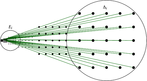
The ball $E_{i}$ solves the preceding problem; $E_{i}$ is large enough to cover all points in $G_{0},\ldots,G_{i-\Theta(\log c)}$. The path from $u\in G_{i}$ directly to $w_{i}\in E_{i}$ and then to any $w\in E_{i}$ has length at most

$$\|uw\|+O(2^{i}/c)\enspace.$$

Furthermore, all of the points in $E_{i}$ are at distance $\Omega(2^{i})$ from all the points in $G_{i}$, so $\|uw\|_{G}/\|uw\|=1+O(1/c)$. Part 3 of the proof of Theorem 1 is dedicated to showing that, in general, the balls $E_{1},\ldots,E_{n^{\prime}}$ help with many pairs of points that would otherwise be problematic.

Example 2: The Importance of Choosing Wisely.

Our second example is intended to illustrate the importance of carefully choosing the representative vertex $w_{i}\in E_{i}$. In this example, there is a dense cluster of $n/2$ points that is contained in some ball $E_{j}$ (see Figure 7). Consider now some $i>j$ such that $r_{i}$ is much greater than $r_{j}$. It is easy to make a configuration of points so that, for some cluster $V_{i}$, the corresponding ball $E_{i}$ contains $E_{j}$ as well as a few other points that are far from $E_{j}$. If one of these points is used as the representative vertex, $w_{i}$, then all $kn/2$ paths from some $u$ in $V_{i}$ to some $w\in E_{j}$ will have to make a detour through $w_{i}$. By repeating this for many different values of $i$, this is enough to produce an average stretch factor significantly larger than 1.

Figure 7: An illustration of why it is important to choose $w_{i}$ carefully. A bad choice (like the one illustrated) leads to a significant detour on the paths from every $u\in V_{i}$ to every $w\in E_{j}$.

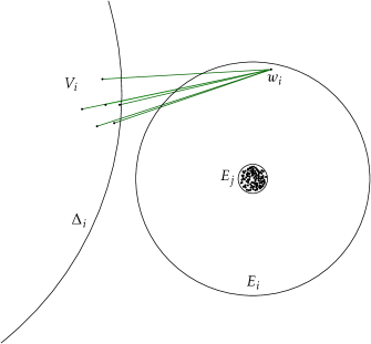
The choice of $w_{i}$ is designed to avoid the preceding problem. In this example, $w_{i}$ would be chosen from the points in $E_{j}$, since $r_{j}<r_{i}$ and $E_{i}$ contains $n/2\geq\epsilon n$ points of $V$. Part 4 of the proof of Theorem 1 is dedicated to showing this careful choice of $w_{i}$ works. In particular, it ensures that, for most pairs of the form $u\in V_{i}$, $w\in E_{i}$,

$$\|uw_{i}\|+O(\|w_{i}w\|)=\|uw\|(1+O(1/c))\enspace.$$

2.4 The Proof

Without further ado, we now prove that $G$ has low average stretch factor.

Theorem 1.

For every constant dimension, $d$, and every set, $V$, of $n<\infty$ points in $\mathbb{R}^{d}$, the graph $G=(V,E)$ described above has $O(n)$ edges and $\operatorname{asf}(G)=1+o_{n}(1)$. More precisely, $\operatorname{asf}(G)=1+O((\log n/n)^{1/(2d+1)})$.

Proof.

That $G$ has $O(n)$ edges follows immediately from its definition.

To upper-bound the average stretch factor of $G$, there are four types of pairs of points, $u\in V_{i}$, $w\in V_{j}$, $j\leq i$, to consider (recall that $\Delta_{1},\ldots,\Delta_{n^{\prime}}$ are ordered so that $r_{j}\leq r_{i}$):

1. pairs that are both from the same set, i.e., where $i=j$;

2. pairs for which $w$ is outside of $D_{i}$;

3. pairs for which $w$ is contained in $D_{i}\setminus E_{i}$; and

4. pairs for which $w$ is contained in $E_{i}\cap D_{i}$.

We consider each of these types of pairs in turn. Our strategy is to study the $\binom{n}{2}$ terms that define $\operatorname{asf}(G)$ in (1). We will show that $o(n^{2})$ of these terms are at most 2 while the remaining terms are at most $1+o_{n}(1)$. Thus,

$$\operatorname{asf}(G)\leq\binom{n}{2}^{-1}\left(2\cdot o(n^{2})+\binom{n}{2}(1+o_{n}(1))\right)=1+o_{n}(1)\enspace.$$

Type 1 Pairs.

Each $V_{i}$, for $i\in\{1,\ldots,n^{\prime}\}$, defines at most $\binom{k}{2}$ Type 1 pairs, so the total number of Type 1 pairs that contribute a term to the sum in (1) is at most

$$\binom{k}{2}\cdot O(n/k)\in O(nk)\enspace.$$

Type 2 Pairs.

For each Type 2 pair $u\in V_{i}$, $w\in V\setminus D_{i}$, there is a path from $u$ to $u_{i}$ in $G_{2}$, then from $u_{i}$ to $u_{j}$ in $G_{1}$ and then finally from $u_{j}$ to $w$ in $G_{2}$ whose length is at most

$$4r_{i}+\|u_{i}u_{j}\|_{G}+4r_{j}\leq(1+1/k^{1/(d-1)})(\|uw\|+16r_{i})\enspace.$$

Furthermore, $\|uw\|\geq(c-1)r_{i}$ since $w$ is outside of $D_{i}$. Therefore, for each Type 2 pair, the term that appears in (1) is of the form

$$\frac{\|uw\|_{G}}{\|uw\|}\leq(1+1/k^{1/(d-1)})(1+O(1/c))=1+O(1/k^{1/(d-1)}+1/c)\enspace.$$

Type 3 Pairs.

The number of Type 3 pairs is no more than

$$k\cdot\sum_{i=1}^{n^{\prime}}|V\cap D_{i}\setminus E_{i}|\enspace.$$

We will prove, by contradiction, that this quantity is $o(n^{2})$. Suppose, for the sake of contradiction, that this is not the case and that

$$\sum_{i=1}^{n^{\prime}}|V\cap D_{i}\setminus E_{i}|\geq\frac{\delta n^{2}}{k}\enspace,$$ (3)

where $\delta>0$ will be determined later. Each term on the left hand side of (3) is at most $n$ and there are $n^{\prime}\leq\alpha n/k$ terms, for some constant $\alpha>0$. We say that a term on the left hand side of (3) is small if it is less than $\delta n/2\alpha$ and large otherwise. The sum of the small terms is at most $\delta n^{2}/2k$ and therefore the sum of the large terms is at least $\delta n^{2}/2k$. Let $J$ be the index set of these large terms. Then

$$\sum_{i\in J}|V\cap D_{i}\setminus E_{i}|\geq\frac{\delta n^{2}}{2k}\enspace.$$

By the pigeonhole principle, there must exist some point $w^{*}\in V$ such that there are at least $\delta n/2k$ indices $i\in J$ such that $w^{*}\in V\cap D_{i}\setminus E_{i}$. To summarize the discussion so far: There exists a point $w^{*}\in V$ and index set, $I\subseteq J$, such that:

1. $w^{*}\in V\cap D_{i}\setminus E_{i}$, for all $i\in I$

2. $|V\cap D_{i}\setminus E_{i}|\in\Omega(\delta n)$, for all $i\in I$; and

3. $|I|\in\Omega(\delta n/k)$.

Suppose, without loss of generality, that the smallest ball, $\Delta_{i}$, with $i\in I$ has unit radius. Partition $I$ into groups $G_{0},G_{1},\ldots$ such that $G_{t}$ contains all indices $i\in I$ such that $\Delta_{i}$ has radius in the interval $[2^{t},2^{t+1})$. We claim that each such group, $G_{t}$, has size $O(c^{d})$. To see why this is so, observe that, for each group $G_{t}$, there exists a point—namely $w^{*}$—that is contained in $|G_{t}|$ balls $D_{i}$ where $i\in G_{t}$. $D_{i}$ has radius at most $c2^{t+1}$. This means that the set of balls

$$\{\Delta_{i}:i\in G_{t}\}$$

is contained in a ball, centered at $w^{*}$, of radius at most $(c+2)2^{t+1}$. Since each ball in this set has radius in $[2^{t},2^{t+1})$, a standard packing argument implies that some point $p\in\mathbb{R}^{d}$ is contained in $\Omega(|G_{t}|/c^{d})$ of these balls. But then Property 4 of $k$-partitions implies that the size of $|G_{t}|/c^{d}\in O(1)$, so $|G_{t}|\in O(c^{d})$.

Thus far, we have shown that each group, $G_{t}$, has size $O(c^{d})$ and the total size of all groups is $|I|\in\Omega(\delta n/k)$. Therefore, there must be at least $\Omega(\delta n/(kc^{d}))$ groups. In particular, we can find $h\in\Omega(\delta n/(kc^{d}\log c))$ groups, $G_{t_{1}},\ldots,G_{t_{h}}$, such that $t_{i+1}\geq t_{i}+2\log c+2$ for each $i\in\{1,\ldots,h-1\}$. By selecting a representative element from each of these groups, we obtain a sequence of indices $i_{1},\ldots,i_{h}$ such that the radius of $\Delta_{i_{j+1}}$ is at least $4c^{d}$ times the radius of $\Delta_{i_{j}}$ for each $j\in\{1,\ldots,h-1\}$.

By choice, $D_{i_{1}}$ contains at least $a\delta n$ elements of $V$, for the constant $a=1/2\alpha$. Also by choice, $D_{i_{2}}\setminus E_{i_{2}}$ contains at least $a\delta n$ elements of $V$. Both $D_{i_{1}}$ and $D_{i_{2}}$ contain the point $w^{*}$. We claim that $E_{i_{2}}$ contains at least $a\delta n$ elements of $V$ as well since there exists a ball, $E_{i_{2}}^{\prime}$, centered at $w^{*}$, of radius $r_{i_{2}}/c>4cr_{i_{1}}$, that contains $D_{i_{1}}$ and therefore contains all the (at least $a\delta n$) points in $D_{i_{1}}$ (see Figure 8). The ball $E_{i_{2}}$ was chosen to contain as many elements of $V$ as possible, so it contains at least as many elements as $E_{i_{2}}^{\prime}$. Therefore, $D_{i_{2}}\cup E_{i_{2}}$ contains at least $2a\delta n$ points of $V$.

Figure 8: $D_{i_{2}}\cup E_{i_{2}}$ contains at least $2an$ points of $V$.

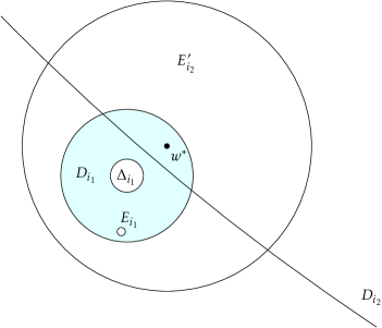
We can now argue similarly to show that $E_{i_{3}}$ contains at least $2a\delta n$ points of $V$ so $D_{i_{3}}\cup E_{i_{3}}$ contains at least $3a\delta n$ points of $V$. In general, this argument shows that $D_{i_{h}}\cup E_{i_{h}}$ contains at least $ha\delta n$ points of $V$. But this yields a contradiction for $h>1/a\delta$, since $V$ contains only $n$ points. To obtain this contradiction, our choice of $\delta$, $c$, and $k$ must satisfy

$$h\in\Omega\left(\frac{\delta n}{kc^{d}\log c}\right)\geq\frac{1}{a\delta}$$

which is satisfied by any choice of $\delta$, $c$, and $k$ such that

$$\frac{\delta^{2}n}{kc^{d}\log c}\geq\frac{C}{a}$$

for some sufficiently large constant $C$. In particular, the value

$$\delta=\sqrt{\frac{Ckc^{d}\log c}{an}}$$

works. So the total number of terms of the sum in (1) contributed by Type 3 pairs is at most

$$\delta n^{2}\in O\left(\sqrt{kn^{3}c^{d}\log c}\right)\enspace.$$

Type 4 Pairs.

Let $\beta>0$ be a constant whose value will be discussed later. We say that a Type 4 pair of points $u\in V_{i}$, $w\in E_{i}\cap D_{i}$ is a bad pair if

$$\|uw_{i}\|+2\|w_{i}w\|\geq(1+\beta/c)\|uw\|\enspace,$$

and otherwise it is a good pair. For any good pair $(u,w)$,

$$\frac{\|uw\|_{G}}{\|uw\|}=1+O(1/c)\enspace,$$

so we can focus our study on bad pairs. To upper-bound the number of bad pairs we will assume, for the sake of contradiction, that the number of bad pairs is at least $\epsilon n^{2}$.

Let $b_{i}$ denote the number of bad pairs $(u,w)$ with $u\in V_{i}$ and $w\in E_{i}\cap D_{i}$. Then, by assumption,

$$\sum_{i=1}^{n^{\prime}}b_{i}\geq\epsilon n^{2}\enspace.$$

Applying the same reasoning used to study Type 3 pairs, we can find a point $w^{*}\in V$ and a set of indices $i_{1},\ldots,i_{\ell}$ such that

1. $w^{*}\in E_{i_{j}}$, for all $j\in\{1,\ldots,\ell\}$;

2. $b_{i_{j}}\in\Omega(\epsilon kn)$, for all $j\in\{1,\ldots,\ell\}$; and

3. $\ell\in\Omega(\epsilon n/k)$.

Assume that the indices $i_{1},\ldots,i_{\ell}$ are ordered so that $r_{i_{j}}\leq r_{i_{j+1}}$ for all $j\in\{1,\ldots,\ell-1\}$. Consider the sequences $E^{\prime}_{i_{1}},\ldots,E^{\prime}_{i_{\ell}}$, where each $E^{\prime}_{i_{j}}$ is the ball of radius $2r_{i_{j}}/c$ centered at $w^{*}$. Recall that the radius of $E_{i_{j}}$ is $r_{i_{j}}/c$ and $w^{*}\in E_{i_{j}}$, so that $E^{\prime}_{i_{j}}\supset E_{i_{j}}$, for each $j\in\{1,\ldots,\ell\}$.

The plan for the rest of the proof is as follows: We will find an annulus $A=E^{\prime}_{i_{j^{*}+t+C}}\setminus E^{\prime}_{i_{j^{*}}}$ that does not contain very many points of $V$. We will then use the fact that $A$ does not contain many of points of $V$ and Property 5 of $k$-partitions to prove that, for some index $j\in\{j^{*},\ldots,j^{*}+t\}$, $b_{i_{j}}<D\epsilon kn$ for any constant $D>0$. This yields the desired contradiction, since $i_{1},\ldots,i_{\ell}$ were chosen so that $b_{i_{j}}\in\Omega(\epsilon kn)$ for every $j\in\{1,\ldots,\ell\}$.

To begin, we fix some positive integers $C\in O(1)$ and $t<\ell-C$ to be specified later. For each $j\in\{2,\ldots,\ell\}$, let $n_{i_{j}}=|E^{\prime}_{i_{j}}\cap V\setminus E^{\prime}_{i_{j-1}}|$. We have that $\sum_{i=2}^{\ell}n_{i_{j}}\leq n$ and $\ell\in\Omega(\epsilon n/k)$. Using these two bounds, a simple averaging argument is sufficient to show that there must exist an index $j^{*}\in\{1,\ldots,\ell-t-C\}$ such that

$$\sum_{j=j^{*}+1}^{j^{*}+t+C}n_{i_{j}}=|V\cap E^{\prime}_{i_{j^{*}+t+C}}\setminus\mathrm{E}^{\prime}_{i_{j^{*}}}|\in O((t+C)k/\epsilon)=O(tk/\epsilon)\enspace.$$ (4)

The careful choice of each $w_{i}\in E_{i}$ implies the following claim, whose proof is deferred until later.

Claim 1.

For every $j\in\{j^{*}+1,\ldots,j^{*}+t\}$, every $u\in V_{i_{j}}$, and every $w\in E_{i_{j}}\cap E^{\prime}_{i_{j^{*}}}\cap V$, $G$ contains a path of length at most $\|uw\|+O(r_{i_{j^{*}}}/c)$.

Figure 9: The number of points in $E$ that are assigned to $\Delta_{i_{j^{*}}},\ldots,\Delta_{i_{j^{*}+t}}$ is only $O(k)$.

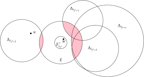
Refer to Figure 9. Let $E$ denote the ball centered at $w^{*}$ and having radius $r_{i_{j^{*}}}=c\cdot\operatorname{radius}(E_{i_{j^{*}}})$. Note that any point $u\not\in E$ is at distance at least $(1-2/c)r_{i_{j^{*}}}$ from any point $w\in E^{\prime}_{i_{j^{*}}}$. Therefore, by Claim 1, for any $w\in E_{i_{j}}\cap E^{\prime}_{i_{j^{*}}}\cap V$, any $j\in\{j^{*}+1,\ldots,j^{*}+t\}$ and any $u\in V_{i_{j}}\setminus E$,

$$\frac{\|uw\|_{G}}{\|uw\|}=1+O(1/c)\enspace.$$

In other words, by choosing an appropriate constant $\beta$ in the definition of bad pairs, $u$ can not form a bad pair with a point $w\in E^{\prime}_{i_{j^{*}}}$ unless $u$ is contained in $E$.

Next we will upper-bound $\sum_{j=j^{*}+1}^{j^{*}+t}b_{i_{j}}$, the number of bad pairs, $(u,w)$, with $u\in V_{i_{j}}$, $w\in E_{i_{j}}$, and $j\in\{j^{*}+1,\ldots,j^{*}+t\}$. From the preceding discussion, each such pair falls into at least one of the two following categories:

1. Category A: $u\in E$. To bound the number of these pairs, consider the balls $\Delta_{i_{j^{*}+1}},\ldots,\Delta_{i_{j^{*}+t}}$. Each of these balls has radius at least $r_{i_{j^{*}}}=\operatorname{radius}(E)$. Therefore, Property 5 of $k$-partitions implies that

   $$\left|\bigcup_{j=j^{*}+1}^{j^{*}+t}V_{i_{j}}\cap E\right|\in O(k)$$

   Each $u$ in $V_{i_{j}}\cap E$ takes part in at most $O(n)$ bad pairs, so the number of bad pairs of this form is $O(kn)$.

2. Category B: $w\not\in E^{\prime}_{i_{j^{*}}}$. By (4), the number of points that are not in $E^{\prime}_{i_{j^{*}}}$ but still in some $E_{i_{j}}\subset E^{\prime}_{i_{j}}$ for $j\in\{j^{*}+1,\ldots,j^{*}+t\}$ is $O(tk/\epsilon)$. Each such point, $w$, forms a bad pair with at most $tk$ different values of $u$—namely the elements of $V_{i_{j^{*}}+1},\ldots,V_{i_{j^{*}+t}}$. Therefore, the number of bad pairs in this category is at most $O((tk)^{2}/\epsilon)$.

Thus, we have

$$\sum_{j=j^{*}+1}^{j^{*}+t}b_{i_{j}}\in O(kn+(tk)^{2}/\epsilon)\enspace.$$ (5)

On the other hand, the indices $i_{1},\ldots,i_{\ell}$ are chosen so that $b_{i_{j}}\in\Omega(\epsilon kn)$, for every $j\in\{1,\ldots,\ell\}$. Therefore

$$\sum_{j=j^{*}+1}^{j^{*}+t}b_{i_{j}}\in\Omega(t\epsilon kn)\enspace.$$ (6)

Equating the right hand sides of (5) and (6), we obtain

$$C_{1}t\epsilon kn\leq C_{2}(kn+(tk)^{2}/\epsilon)\enspace,$$

for some constants $C_{1}$ and $C_{2}$. This yields a contradiction when

$$t>D/\epsilon$$

and

$$\epsilon\geq D\sqrt{\frac{tk}{n}}\enspace,$$

for some sufficiently large constant $D$. Setting $t=D/\epsilon$ leaves only the condition

$$\epsilon\geq D^{2/3}\left(\frac{k}{n}\right)^{1/3}\enspace.$$

Thus, there exists some constant $D_{0}$ such that the total number of bad Type 4 pairs is at most

$$\epsilon n^{2}\enspace,$$

provided that $\epsilon\geq D_{0}(k/n)^{1/3}$.

All that remains in handling Type 4 pairs is to prove Claim 1.

Proof of Claim 1.

Let $u$ by any point in $V_{i_{j}}$, for any $j\in\{j^{*}+1,\ldots,j^{*}+t\}$. Since there is an edge joining $u$ and $w_{i_{j}}$ and $\|w^{*}w\|\leq 2r_{i_{j^{*}}}/c$, there is a path from $u$ to $w$ of length at most

$$\|uw\|_{G} \leq\|uw_{i_{j}}\|+2\|w_{i_{j}}w^{*}\|+2\|w^{*}w\|$$

$$\leq\|uw\|+\|ww_{i_{j}}\|+2\|w_{i_{j}}w^{*}\|+4r_{i_{j}^{*}}/c$$

$$\leq\|uw\|+\|ww^{*}\|+3\|w_{i_{j}}w^{*}\|+4r_{i_{j}^{*}}/c$$

$$\leq\|uw\|+3\|w_{i_{j}}w^{*}\|+6r_{i_{j}^{*}}/c\enspace,$$

so it is sufficient to prove that $\|w^{*}w_{i_{j}}\|\in O(r_{i_{j^{*}}}/c)$. If $w_{i_{j}}=w^{*}$, then we are done, so assume $w_{i_{j}}\neq w^{*}$. Since $w^{*}\in E_{i_{j}}$ but was not chosen to act as $w_{i_{j}}$, there must exist some index $i^{\prime}$ such that $E_{i^{\prime}}\cap E_{i_{j}}\neq\emptyset$, $|E_{i^{\prime}}\cap V|\geq\epsilon n$, $r_{i^{\prime}}\leq r_{i_{j^{*}}}$, and $w_{i_{j}}\in E_{i^{\prime}}$. (Note for later: This is the only place in the entire proof of Theorem 1 where the choice of $w_{i_{j}}$ matters.)

There are two cases to consider:

1. If $E^{\prime}_{i_{j^{*}}}$ intersects $E_{i^{\prime}}$, then (see Figure 10)

   $$\|w^{*}w_{i_{j}}\|\leq 2r_{i_{j^{*}}}/c+2r_{i^{\prime}}/c\leq 4r_{i_{j^{*}}}/c\in O(r_{i_{j^{*}}}/c)\enspace,$$

   and we are done.

   

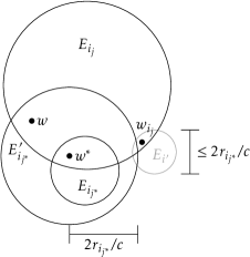
   Figure 10: If $E_{i^{\prime}}$ intersects $E^{\prime}_{i_{j}^{*}}$ then $\|w^{*}w_{i_{j}}\|\leq 4r_{i_{j^{*}}}/c$.

2. If $E_{i^{\prime}}$ and $E^{\prime}_{i_{j^{*}}}$ are disjoint, then we claim that $E_{i^{\prime}}\subset E^{\prime}_{i_{j^{*}+t+C}}$ (see Figure 11). To see why this is so, we argue that, when $C$ is a sufficiently large constant,

   $$r_{i_{j^{*}+t+C}}>2r_{i_{j^{*}+t}}\geq 2r_{i_{j}}\enspace.$$ (7)

   This implies that $E_{i^{\prime}}\subset E^{\prime}_{i_{j^{*}+t+C}}$ since every point in $E_{i^{\prime}}$ is at distance at most $4r_{i_{j}}$ from $w^{*}$ and $E^{\prime}_{i_{j^{*}+t+C}}$ is centered at $w^{*}$ and has radius $2r_{i_{j^{*}+t+C}}>4r_{i_{j}}$.

   To see why the first inequality in (7) holds, we first observe that, for any $i\in\{1,\ldots,n^{\prime}\}$, if any $u\in V_{i}$ and $w\in E_{i}$ form a bad pair, then the distance from $\Delta_{i}$ to $E_{i}$ is less than $r_{i}$. Since each $V_{i_{j}}$ and $E_{i_{j}}$ define at least one pair, this implies that each $\Delta_{i_{j}}$ is contained in a ball of radius $(3+2/c)r_{i_{j}}$ centered at $w^{*}$.

   Now, if $r_{i_{j^{*}+t+C}}<2r_{i_{j^{*}+t}}$, then $\Delta_{i_{j^{*}+t}},\ldots,\Delta_{i_{i_{j^{*}+t+C}}}$ is a set of $C+1$ balls all having radii in $[r_{i_{j^{*}+t}},2r_{i_{j^{*}+t}})$ and that are all contained in a ball of radius $(6+4/c)r_{i_{j^{*}+t}}$ centered at $w^{*}$. Therefore, some point, $p$, in this ball is contained in $\Omega(C)$ of these balls. But then Property 4 of $k$-partitions implies that $C\in O(1)$. Thus, for a sufficiently large constant, $C$, $r_{i_{j^{*}+t+C}}>2r_{i_{j^{*}+t}}$ and $E_{i^{\prime}}\subset E_{i_{j^{*}+t+C}}$, as promised.

   Since $E_{i^{\prime}}$ and $E_{i_{j^{*}}}$ are disjoint and $E_{i^{\prime}}\subset E_{i_{j^{*}+t+C}}$,

   $$|V\cap E_{i_{j^{*}+t+C}}\setminus E_{i_{j^{*}}}|\geq|V\cap\mathrm{E}_{i^{\prime}}|\geq\epsilon n\enspace.$$

   

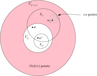
   Figure 11: If $E_{i^{\prime}}$ does not intersect $E^{\prime}_{i_{j}^{*}}$ then $E_{i_{j^{*}+t+C}}\setminus E_{i_{j^{*}}}$ contains at least $\epsilon n$ points.

   But, by definition,

   $$|V\cap E_{i_{j^{*}+t+2\mu}}\setminus E_{i}|\in O(tk/\epsilon)\enspace.$$

   This yields a contradiction when $t<D^{\prime}\epsilon^{2}n/k$, for a sufficiently small constant $D^{\prime}>0$. Note that we have already set $t=D/\epsilon$, so this requires that

   $$D/\epsilon<D^{\prime}\epsilon^{2}n/k\Leftrightarrow\epsilon>\left(\frac{Dk}{D^{\prime}n}\right)^{1/3}\enspace.$$

   Therefore, the condition on $t$ is already contained in the requirement that $\epsilon\geq D_{0}(k/n)^{1/3}$.

This completes the proof of Claim 1. ∎

Finishing Up.

We can now pull everything together to summarize and complete the proof of Theorem 1.

1. The number of Type 1 pairs is at most $O(kn)$.

2. For each Type 2 pair, $(u,w)$, $\|uw\|_{G}/\|uw\|\leq 1+O(1/k^{1/(d-1)}+1/c)$.

3. The number of Type 3 pairs is at most $O(\sqrt{kn^{3}c^{d}\log c})$.

4. For each good Type 4 pair, $(u,w)$, $\|uw\|_{G}/\|uw\|\leq 1+O(1/c)$.

5. The number of bad Type 4 pairs is at most $O(\epsilon n^{2})$ provided that $\epsilon\in\Omega((k/n)^{1/3})$.

Putting all these together, we obtain

$$\operatorname{asf}(G)=1+O\left(1/k^{1/(d-1)}+1/c+\binom{n}{2}^{-1}\left(kn+\sqrt{kn^{3}c^{d}\log c}+\epsilon n^{2}\right)\right)\enspace.$$ (8)

Taking

$$\epsilon=(k/n)^{1/3}\enspace,$$

$$k=\left(\frac{n}{\log n}\right)^{(d-1)/(2d+1)}$$

and

$$c=\left(\frac{n}{\log n}\right)^{1/(2d+1)}$$

yields

$$\operatorname{asf}(G)=1+O\left(\left(\frac{\log n}{n}\right)^{1/(2d+1)}\right)\enspace.$$

(The $O(kn/\binom{n}{2})$ term and the $\epsilon n^{2}/\binom{n}{2}$ term are dominated by the three other terms, which are all $O((\log n/n)^{1/(2d+1)})$.) ∎

Remark 1.

In the next section, efficient algorithms will require that $\epsilon=(\log^{\kappa}n)/k$ for some constant $\kappa\geq 0$. Since the bound on the average stretch factor requires that $\epsilon\in\Omega((k/n)^{1/3})$, this implies that the value of $k$ must be at most $n^{1/4}$. The following table shows the optimal choices of $k$ and $c$ for different dimensions, $d$:

$d$	$k$	$c$	$\operatorname{asf}(G)$
$2$	$(n/\log n)^{1/5}$	$(n/\log n)^{1/5}$	$1+O((\log^{5\kappa+1}n/n)^{1/5})$
$\geq 3$	$n^{1/4}$	$(\log n/n^{3/4})^{1/(d+2)}$	$1+O(1/n^{1/(4d-4)})$

3 Algorithms

In this section, we discuss efficient algorithms for computing a graph $G=(V,E)$ that has low average stretch factor, given the point set $V\subset\mathbb{R}^{d}$. We first present a fairly straightforward adaptation of the construction given in the preceding section that yields an $O(n\log^{d}n)$ time algorithm. We then show that some refinements of this algorithm lead to an $O(n\log n)$ time algorithm.

Our algorithms are randomized. Throughout this section, we say that an event within an algorithm happens with high probability if the event occurs with probability at least $1-O(n^{\alpha})$ and $\alpha$ can be made into an arbitrarily large constant by increasing the running time of the algorithm by a constant factor.

3.1 A Simple Algorithm

For ease of exposition, we start with a simple algorithm that is relatively faithful to the proof of Theorem 1.

Theorem 2.

For every constant dimension, $d$, and every set, $V$, of $n<\infty$ points in $\mathbb{R}^{d}$, there exists a randomized $O(n\log^{d}n)$ time algorithm that constructs a graph $G^{\prime}=(V,E)$ that has $O(n)$ edges and, with high probability,

$$\operatorname{asf}(G^{\prime})=\begin{cases}1+O((\log n/n)^{1/5})&\text{for $d=2$}\\ 1+O(1/n^{1/(4d-4)})&\text{for $d\geq 3$}\\ \end{cases}$$

Proof.

Throughout this proof, a box is an axis-aligned box of the form $[a_{1},b_{1}]\times\cdots\times[a_{d},b_{d}]$ and we call this a square box if $b_{i}-a_{i}=b_{j}-a_{j}$ for all $i,j\in\{1,\ldots,d\}$. As before, $L(B)$ denotes the length of the longest side of the box, $B$. The graph $G^{\prime}$ constructed by our algorithm is similar to the graph, $G$, described in the previous section, except for three major differences:

1. Every element in $G$ that is defined in terms of a ball is now defined in terms of a square box. In particular,

   1. $\Delta_{1},\ldots,\Delta_{n^{\prime}}$ are minimal square boxes that contain the corresponding boxes defined by nodes of the fair-split tree;

   2. $D_{1},\ldots,D_{n^{\prime}}$ are square boxes where each $D_{i}$ is a square box of side-length $cL(\Delta_{i})$ centered at the center of $\Delta_{i}$; and

   3. $E_{1},\ldots,E_{n^{\prime}}$ are square boxes where each $E_{i}$ is a square box of side-length $L(\Delta_{i})/c$ that intersects $D_{i}$.

2. The box $E_{i}$ does not perfectly maximize the number of points it contains. Instead, we guarantee that, if there exists any box of side-length $L(\Delta_{i})/2c$ that intersects $D_{i}$ and contains $m\geq\epsilon n$ points of $V$, then $E_{i}$ is chosen so that it contains at least $m$ points of $V$.

3. We change the value of $\epsilon$ to $\epsilon=1/k$ and use the values of $c$ and $k$ given in Remark 1.

It is straightforward, but tedious, to check that the proof of Theorem 1 using these new definitions of $\Delta_{i}$, $D_{i}$, and $E_{i}$ shows that the graph $G^{\prime}$ satisfies the requirements of the theorem. What remains is to show how the graph $G^{\prime}$ can be constructed in $O(n\log^{d}n)$ time.

As described in the proof of Lemma 1, computing the fair-split tree, and the resulting $\Delta_{1},\ldots,\Delta_{n^{\prime}}$, $V_{1},\ldots,V_{n^{\prime}}$, $u_{1},\ldots,u_{n^{\prime}}$ and $D_{1},\ldots,D_{n^{\prime}}$ is easily accomplished in $O(n\log n)$ time. The 2-spanner of the points in $V$ can be constructed in $O(n\log n)$ time using any of several different possible methods [8, 18, 20]. An algorithm of Ruppert and Seidel [17] can, for any $\gamma>0$, construct a $(1+\gamma)$-spanner of $n^{\prime}$ points in $\mathbb{R}^{d}$ that has $O((1/\gamma)^{d-1}n^{\prime})$ edges in $O((1/\gamma)^{d-1}n^{\prime}\log^{d-1}n^{\prime})$ time. Using this algorithm with $\gamma=1/k^{1/(d-1)}$, the $(1+1/k^{1/(d-1)})$-spanner of the $n^{\prime}$ points in $H$ can be constructed in time

$$O(kn^{\prime}\log^{d-1}n^{\prime})=O(n\log^{d-1}n)\enspace.$$

All that remains is to show how to compute $E_{1},\ldots,E_{n^{\prime}}$ and $w_{1},\ldots,w_{n^{\prime}}$ efficiently.

The reason for moving from balls to square boxes is that boxes allow for the use of range trees [6, 15]. Range trees allow us to preprocess, using $O(n\log^{d-1}n)$ time and space, a set of $n$ points in $\mathbb{R}^{d}$ so that, for any query box, $B$, we can find, in $O(\log^{d-1}n)$ time: (1) the number of points in $B$, or (2) the point with minimum index in $B$. Furthermore, by using a box-point duality that maps square boxes in $\mathbb{R}^{d}$ onto points in $\mathbb{R}^{d+1}$, a set of square boxes in $\mathbb{R}^{d}$ can be preprocessed, using $O(n\log^{d}n)$ time and space, so that, for any query point $p\in\mathbb{R}^{d}$, we can, in $O(\log^{d}n)$ time, determine the index of the smallest box that contains $p$.

Our first task is to find the boxes $E_{1},\ldots,E_{n^{\prime}}$ and for this we use random sampling. Let $D^{\prime}_{i}$ be the square box that is centered at the center of $\Delta_{i}$ and has side-length $(c+1/2c)L(\Delta_{i})$. We repeatedly select a random point $u\in V$. If $u$ is not in $D^{\prime}_{i}$, then we discard it. Otherwise, we count the number of points in the box, $E(u)$, that is centered at $u$ and has side length $L(\Delta_{i})/c$. The sample box containing the maximum number of points is chosen as $E_{i}$. (If all samples were discarded, then we take $E_{i}$ to be any square box of side length $L(\Delta_{i})/c$ that intersects $D_{i}$.)

Let $E^{\prime}_{i}$, be some square box of side length $L(\Delta_{i})/2c$ that intersects $D_{i}$ and that contains the maximum number of points in $V$. Suppose, furthermore, that $|E^{\prime}_{i}\cap V|\geq\epsilon n$ (since this is the only case in which we make any guarantees about $E_{i}$). If we repeat the above sampling procedure $\alpha\ln n/\epsilon$ times, then the probability that none of our samples is a point in $|E^{\prime}_{i}\cap V|$ is at most

$$(1-\epsilon)^{\alpha\ln n/\epsilon}\leq 1/e^{\alpha\ln n}=1/n^{\alpha}\enspace.$$

Therefore, with high probability, at least one of our sample points, $u$, is in $E^{\prime}_{i}$. In this case, $E(u)$ contains $E^{\prime}_{i}$, so we obtain a box, $E_{i}$ that intersects $D_{i}$ and contains $E^{\prime}_{i}$.

By storing the points of $V$ in a range tree, we can therefore identify the boxes $E_{1},\ldots,E_{n^{\prime}}$ in time

$$O(n^{\prime}(\log n/\epsilon)\log^{d-1}n)=O\left(\frac{n\log^{d}n}{\epsilon k}\right)=O(n\log^{d}n)\enspace.$$

Let $E\subseteq\{E_{1},\ldots,E_{n^{\prime}}\}$ be the subset of boxes that contain at least $\epsilon n$ points of $V$. By using the point-box duality, we can store $E$ in a range tree so that, for each point $w\in V$, we can determine the index, $i(w)$, of the smallest box that contains at least $\epsilon n$ points of $V$ and contains $w$. Building the range tree for (the duals of) $E_{1},\ldots,E_{n^{\prime}}$ takes $O(n^{\prime}\log^{d}n)\subset O(n\log n)$ time and searching this range tree for each point $w\in V$ takes time

$$O(n\log^{d}n)\enspace.$$

Finally, we can store the point/index pairs $(u,i(u))$, for all $u\in V$, in a range tree so that, for each box, $E_{i}$, we can find a point $w_{i}\in E_{i}$ that minimizes $i(u)$. Building this range tree takes $O(n\log^{d-1}n)$ time and the queries on this tree take $O(n^{\prime}\log^{d-1}n)\subset O(n\log^{d-1}n)$ time. ∎

3.2 A Faster Algorithm

In the preceding section we gave an $O(n\log^{d}n)$ time algorithm. In this section, we show that the running time can be reduced to $O(n\log n)$ with only a small increase in the average stretch factor.

Theorem 3.

For every constant dimension, $d$, and every set, $V$, of $n<\infty$ points in $\mathbb{R}^{d}$, there exists a randomized $O(n\log n)$ time algorithm that constructs a graph $G^{\prime\prime}=(V,E)$ that has $O(n)$ edges and, with high probability,

$$\operatorname{asf}(G^{\prime\prime})=\begin{cases}1+O((\log^{6}n/n)^{1/5})&\text{for $d=2$}\\ 1+O(\log^{(d-2)/(d-1)}n/n^{1/(4d-4)})&\text{for $d\geq 3$}\end{cases}$$

Proof.

The construction of $G^{\prime\prime}$ is similar to the construction of $G^{\prime}$ described in the proof of Theorem 2. In the construction of $G^{\prime}$, there are three issues that lead to a running-time of $\omega(n\log n)$: (1) the construction of the $(1+(1/k)^{1/(d-1)})$-spanner of $H$ takes $\Theta(n\log^{d-1}n)$ time; (2) the sampling algorithm used to find the boxes $E_{1},\ldots,E_{n^{\prime}}$ that contain at least $\epsilon n$ points takes $\Theta(n\log^{d}n)$ time; and (3) determining the index, $i(u)$, of each point $u\in V$ takes $\Theta(n\log^{d}n)$ time. We address each of these issues in turn:

1. We only construct a $(1+(\log^{d-2}n/k)^{1/(d-1)})$-spanner of $H$. Using the algorithm of Ruppert and Seidel, the construction of this spanner takes only $O(n\log n)$ time. This modification increases the average stretch factor of the resulting graph, so that the lower-order term increases by a factor of $\log^{(d-2)/(d-1)}n$.

2. The sampling process used to find $E_{1},\ldots,E_{n^{\prime}}$ has two phases. In Phase 1, a range tree is constructed that contains the points of $V$. In Phase 2, $O(n^{\prime}\log n/\epsilon)$ queries are performed on this range tree.

   Phase 1 takes $O(n\log^{d-1}n)$ time. To speed up Phase 1, we instead construct a range tree, $T_{1}$, on a Bernoulli sample $V^{\prime}\subseteq V$ where each point is sampled independently with probability $p=\alpha/\log^{d-2}n$. A standard application of Chernoff’s Bounds [4, Appendix A.1] shows that, with high probability,

   1. $T_{1}$ can be constructed in $O(n\log n)$ time;

   2. for all boxes, $B$, with $|B\cap V|\geq\epsilon n$,

      $$(1/2)|B\cap V|\leq|B\cap V^{\prime}|/p\leq 2|B\cap V|\enspace;$$

   3. for all boxes, $B$, with $|B\cap V|\leq\epsilon n/2$,

      $$|B\cap V^{\prime}|/p\leq\epsilon n\enspace.$$

   Properties (b) and (c) above ensure that the quantity $|B\cap V^{\prime}|/p$, which can be computed in $O(\log^{d-1}n)$ time using $T_{1}$, is an accurate enough estimate of $|B\cap V|$.

   Phase 2 requires sampling $\alpha n^{\prime}\ln n/\epsilon$ points and, for each sample point, $u$, counting the number of points of $V$ in some box centered at $u$. By increasing the value of $\epsilon$ from $\epsilon=1/k$ to $\epsilon=\log^{d-1}n/k$, this counting can be done in $O(n\log n)$ time using $T_{1}$. Remark 1, with the value $\kappa=d-1$, explains why this new choice of $\epsilon$ does not increase the average stretch factor for $d\geq 3$, and increases it by a factor of $\log n$ for $d=2$.

3. To determine the index, $i(u)$, of each point $u\in V$, we first construct a range tree, $T_{2}$ for (the duals of) some boxes in $\{E_{1},\ldots,E_{n^{\prime}}\}$. In $T_{2}$, we include every box, $B\in\{E_{1},\ldots,E_{n^{\prime}}\}$ such that $|B\cap V^{\prime}|/p\geq\epsilon n$. From the preceding discussion, with high probability, $T_{2}$ then contains only boxes, $B$ such that $|B\cap V|\geq\epsilon n/2$ and $T_{2}$ includes every box, $B$ such that $|B\cap V|\geq 2\epsilon n$.

   Determining which boxes to include in $T_{2}$ requires $n^{\prime}$ queries in $T_{1}$, so this takes $O(n^{\prime}\log^{d-1}n)\subset O(n\log n)$ time. Building the tree $T_{2}$ takes $O(n^{\prime}\log^{d}n)\subset O(n\log n)$ time. At this point, we would like to use $T_{2}$ to compute $i(w)$ for every point $w\in V$, but this would take $\Omega(n\log^{d}n)$ time. Instead, we take another sample, $V^{\prime\prime}\subseteq V$ of size $n/\log^{d-1}n$ and compute $i(w)$ for each $w\in V^{\prime\prime}$. This takes only $O(n\log n)$ time.

   Finally, we put each pair $(u,i(u))$ for each $u\in V^{\prime\prime}$ into another range tree $T_{3}$. This takes only $O(|V^{\prime\prime}|\log^{d-1}n)=O(n)$ time. We then query $T_{3}$ with each box in $\{E_{1},\ldots,E_{n^{\prime}}\}$ to determine the point $w_{i}\in E_{i}\cap V^{\prime\prime}$ that minimizes $i(w_{i})$. This takes only $O(n^{\prime}\log^{d-1}n)\subset O(n\log n)$ time.

   It remains to argue that the point, $w_{i}$, which minimizes $i(w_{i})$ over all $w_{i}\in E_{i}\cap V^{\prime\prime}$ is a good-enough replacement for the point, $w_{i}^{*}$, that minimizes $i(w_{i}^{*})$ over all $w_{i}^{*}\in E_{i}\cap V$. To establish this, it is necessary to revisit the proof of Theorem 1. The only place in the proof of Theorem 1 in which the choice of $w_{i}$ plays a role is in counting the number of bad Type 4 pairs.

   Recall that this part of the proof of Theorem 1 assumes that the number of bad Type 4 pairs is greater than $\epsilon n^{2}$ and uses this assumption to derive a contradiction. In particular, the proof shows the existence of a point $w^{*}$ that satisfies Conditions B1–B3. Walking through the proof, we see that it continues to work if there is any point $w^{*}\in V^{\prime\prime}$ that satisifies Conditions B1–B3. In particular, $w^{*}\in V^{\prime\prime}$ is sufficient to establish Claim 1, which is the only place in the entire proof of Theorem 1 that makes use of the fact that $w_{i}$ minimizes $i(w_{i})$ over all $w_{i}\in E_{i}$.

   In the proof of Theorem 1, the existence of $w^{*}$ is established by the pigeonhole principle; we have subsets $S_{1},\ldots,S_{r}$ of $V$ whose total size is $\Omega(\epsilon n^{2}/k)$ and we conclude that some element $w^{*}\in V$ must occur in $\Omega(\epsilon n/k)$ subsets. However, the number of subsets, $r$, is only $O(n/k)$. We can therefore make a stronger conclusion: There are $\Omega(\epsilon n)$ elements $w^{*}\in V$ such that $w^{*}$ appears in $\Omega(\epsilon n/k)$ subsets.

   Thus, there exists a set $W^{*}\subseteq V$ of size $\Omega(\epsilon n)$ such that any point $w^{*}\in W^{*}$ is good enough to derive the contradiction required to bound the number of bad Type 4 pairs. If even one point of $W^{*}$ appears in $V^{\prime\prime}$, then the bound on the number of bad Type 4 pairs holds. The sample, $V^{\prime\prime}$, is taken after the boxes $E_{1},\ldots,E_{n^{\prime}}$ and therefore after $W^{*}$ has been defined, so $V^{\prime\prime}$ and $W^{*}$ are independent. The size of $W^{*}$ is $\Omega(\epsilon n)$, so the probability that a randomly chosen element of $V$ is in $W^{*}$ is $\Omega(\epsilon)$. The sample $V^{\prime\prime}$ contains $n/\log^{d-1}n$ randomly chosen elements of $V$, so the probability that $V^{\prime\prime}$ and $W^{*}$ are disjoint is at most

   $$(1-\Omega(\epsilon))^{n/\log^{d-1}n}\leq\exp(-\Omega(\epsilon n/\log^{d-1}n))\leq n^{\alpha}\enspace,$$

   for any constant $\alpha>0$ and all sufficiently large values of $n$. Therefore, with high probability $V^{\prime\prime}$ contains at least one element of $W^{*}$ and the number of bad Type 4 pairs is at most $\epsilon n^{2}$.

This completes the proof of Theorem 3. ∎

4 Lower Bounds

Next, we prove a simple lower-bound which shows that our bound on the average stretch factor is at least of the right flavour: Combined with the upper-bound of Theorem 1, the following result shows that the optimal bound is $1+O(1/n^{\delta})$ for some $\delta\in(1/(2d+1),1/2]$.

Theorem 4.

For every positive integer, $n$, there exists a set, $V$, of $n$ points in $\mathbb{R}^{2}$, such that every geometric graph, $G$, with vertex set $V$ and having $O(n)$ edges has $\operatorname{asf}(G)\geq 1+\Omega(1/\sqrt{n})$.

Proof.

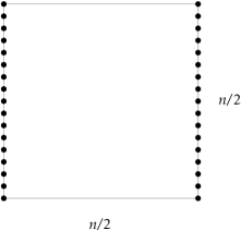
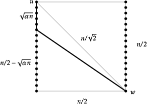
For simplicity, we assume $n$ is even. The point set, $V$, has its points evenly distributed on two opposite sides of a square. The point set $V=A\cup B$, where

$$A=\{(0,i):i\in\{1,\ldots,n/2\}\}$$

and

$$B=\{(n/2,i):i\in\{1,\ldots,n/2\}\}$$

is an example (see Figure 12.a).

(a)	(b)

Figure 12: The lower-bound (a) point set for Theorem 4, and (b) the best-case ratio $\|uw\|_{G}/\|uw\|$ for a pair $(u,w)$ that is not covered by any edge.

Let $G$ be any graph with vertex set $V$. We say that an edge $uw$ with $u\in A$ and $w\in B$ covers the set of pairs

$$\{\left(u+(0,i),w+(0,j)\right):i,j\in\{-\sqrt{\alpha n},\ldots,\sqrt{\alpha n}\}\}$$

for some constant $\alpha$ to be discussed later. Thus, any edge of $G$ covers at most $4\alpha n$ pairs in $A\times B$.

Next, observe that if some pair of points $u\in A$ and $w\in B$ is not covered by any edge of $G$, then a straightforward minimization argument (see Figure 12.b) shows that

$$\frac{\|uw\|_{G}}{\|uw\|} \geq\frac{\sqrt{\alpha n}+\sqrt{(n/2)^{2}+(n/2-\sqrt{\alpha n})^{2}}}{n/\sqrt{2}}$$

$$=\frac{\sqrt{\alpha n}+\sqrt{n^{2}/2-\sqrt{\alpha}n^{3/2}+\alpha n/2}}{n/\sqrt{2}}$$

$$\geq\frac{\sqrt{\alpha n}+n/\sqrt{2}-\sqrt{\alpha n/2}}{n/\sqrt{2}}$$ (9)

$$\geq 1+\Omega(1/\sqrt{n})\enspace.$$

(Inequality (9) is obtained by comparing $\left(\sqrt{n^{2}/2-\sqrt{\alpha}n^{3/2}+\alpha n/2}\right)^{2}$ and $\left(n/\sqrt{2}-\sqrt{\alpha n/2}\right)^{2}$.) If $G$ has $m\in O(n)$ edges, then we select $\alpha\leq\binom{n}{2}/(8mn)$ so that

$$m4\alpha n\leq\frac{\binom{n}{2}}{2}$$

In this way, at least half of the $\binom{n}{2}$ pairs of points in $V$ are not covered by any edge and therefore,

$$\operatorname{asf}(G)\geq 1+\binom{n}{2}^{-1}\cdot\frac{\binom{n}{2}}{2}\cdot\Omega(1/\sqrt{n})=1+\Omega(1/\sqrt{n})\enspace.\qed$$

We remark that the proof of Theorem 4 is easily modified to provide a tradeoff between the number of edges of $G$ and the average stretch factor. In particular, if $G$ has $m\in o(n^{2})$ edges, then

$$\operatorname{asf}(G)\geq 1+\Omega(1/\sqrt{m})\enspace.$$

5 Discussion

We have shown that, for any set, $V$, of $n$ points in $\mathbb{R}^{d}$, we can construct, in $O(n\log n)$ time, a graph on $V$ whose average stretch factor is $1+o_{n}(1)$. Our construction consists of three parts, (1) a 2-spanner, $G_{2}$ of $V$, (2) a $1+o_{n}(1)$-spanner of a subset $H\subset V$ of so-called hubs, and (3) a collection of edges that join all vertices within each group, $V_{i}$, to a single representative vertex, $w_{i}$, within a very dense (compared to $V_{i}$) set of vertices, $E_{i}\cap V$.

5.1 Realistic Networks(?)

We note that, if one has some form of reasonable well-distributed assumption about the points in $V$, like that used by Aldous and Kendall, then it is fairly straightforward to show that the first two parts of our construction are sufficient to obtain an average stretch factor of $1+o_{n}(1)$. The third part of our construction is only required to deal with instances in which there are exponential differences in density of points of $V$. It seems natural to ask whether this part of the construction is necessary in any real-world network or whether the vertices of real-world networks are always well-distributed.

The first two parts of our construction are quite natural and can be recognized in many real-world networks. The most common (though admittedly, imperfect) example is road networks where individual buildings are interconnected by roads, which very often form a partial grid (a $\sqrt{2}$-spanner). The cities, towns, and villages, containing these buildings are themselves interconnected by a relatively fast, and fairly direct, system of highways.

The third part of our construction seems less natural. In road networks, this part of the construction would correspond to densely-populated areas that have several direct routes to them from well-separated locations. Since this part of our construction is only required to deal with pathological cases involving inter-point distances that vary exponentially, one might think that it does not appear in real-world networks.

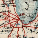
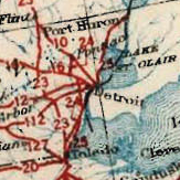
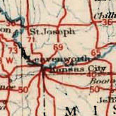
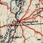
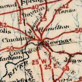
A quick inspection of the U.S. Highway System shows that, even by 1926, there were many direct highway connections to Chicago, Detroit, Kansas City, Memphis, Newport, and other large cities (see Figure 13). These highways were expensive and would have been built unless they added real value to the road network. While this does not correspond perfectly with the third part of our construction, it does suggest that a simple two-level network of clusters, each having a single hub, does not produce real-world networks of sufficient quality; some form of extra augmentation is necessary.

Figure 13: Large cities have many direct routes to them. (Source: Map of the final U.S. Highway system as approved November 11, 1926. This map is in the public domain.)

5.2 Open Problems

Our results leave many areas open for further research. We say that a graph, $G=(V,E)$ has good average stretch if $\operatorname{asf}(G)=1+o_{n}(1)$ and $|E|=O(n)$.

The following open problems have to do with strengthenings of Theorem 1 in which $G$ has additional properties.

Open Problem 1.

Given a point set, $V$, does there always exist a good average stretch graph $G=(V,E)$ whose total edge length is close to that of the minimum spanning tree?

Open Problem 2.

Given a point set, $V$, does there always exist a good average stretch graph $G=(V,E)$ whose maximum degree is bounded by a constant?

Open Problem 3.

Given a point set, $V$, does there always exist a good average stretch graph $G=(V,E)$ that is $k$-fault tolerant? That is, for any set $F\subset V$, $|F|\leq k$, $\operatorname{asf}(G\setminus F)=1+o_{n}(1)$.

Open Problem 4.

Bose et al. [7] define $f(k)$-robust spanners in terms of the (worst-case) stretch factor and their definition extends naturally to average stretch factor. Given a point set, $V$, does there always exist a good average stretch graph $G=(V,E)$ that is $f(k)$-robust, for some reasonable function $f(k)$?

The following question asks if the upper-bound can be proven in a more general setting:

Open Problem 5.

What conditions on a metric space $(V,d)$ are necessary and sufficient so that there always exist a graph $G=(V,E)$, $|E|\in O(n)$ with $\operatorname{asf}(G)=1+o_{n}(1)$? (Here shortest paths in $G$ are measured in terms of the cost of their edges in the metric space.)

It seems likely that some of the techniques used to prove Theorem 1 are applicable to metric spaces of bounded doubling dimension [14, Section 10.13]. Is bounded doubling dimension the weakest possible restriction on the metric space? It is clear that some restrictions on the metric space are required: In the metric space in which all points have unit distance, the average stretch factor of a graph, $G=(V,E)$, having $m$ edges is at least

$$\binom{n}{2}^{-1}\left(m+2\left(\binom{n}{2}-m\right)\right)$$

since, if there is no edge between $u$ and $w$ in $G$, then $\|uw\|_{G}\geq 2$. Therefore any graph with average stretch factor $1+o_{n}(1)$ must have $\binom{n}{2}-o(n^{2})$ edges.

Authors

Vida Dujmović. School of Mathematics and Statistics and Department of Systems and Computer Engineering, Carleton University

Pat Morin and Michiel Smid. School of Computer Scence, Carleton University

References

- [1] I. Abraham, Y. Bartal, H. T.-H. Chan, K. Dhamdhere, A. Gupta, J. M. Kleinberg, O. Neiman, and A. Slivkins. Metric embeddings with relaxed guarantees. In Proceedings of the 46th Annual IEEE Symposium on Foundations of Computer Science (FOCS 2005), pages 83–100. IEEE Computer Society, 2005.
- [2] I. Abraham, Y. Bartal, and O. Neiman. Embedding metrics into ultrametrics and graphs into spanning trees with constant average distortion. In N. Bansal, K. Pruhs, and C. Stein, editors, Proceedings of the Eighteenth Annual ACM-SIAM Symposium on Discrete Algorithms (SODA 2007), pages 502–511. SIAM, 2007.
- [3] D. J. Aldous and W. S. Kendall. Short-length routes in low-cost networks via Poisson line patterns. Advances in Applied Probability, 40(1):1–21, 2008.
- [4] N. Alon and J. H. Spencer. The Probabilistic Method. John Wiley & Sons, Hoboken, third edition, 2008.
- [5] M. A. Bender and M. Farach-Colton. The LCA problem revisited. In Proceedings of Latin American Theoretical Informatics (LATIN 2000), pages 88–94, 2000.
- [6] J. L. Bentley. Multidimensional divide-and-conquer. Communications of the ACM, 23(5):214–228, 1978.
- [7] P. Bose, V. Dujmović, P. Morin, and M. Smid. Robust geometric spanners. In Proceedings of the Twenty-Ninth ACM Symposium on Computational Geometry (SoCG 2013). ACM Press, 2013.
- [8] P. B. Callahan and S. R. Kosaraju. Faster algorithms for some geometric graph problems in higher dimensions. In Proceedings of the 4th ACM-SIAM Symposium on Discrete Algorithms, pages 291–300, 1993.
- [9] P. B. Callahan and S. R. Kosaraju. A decomposition of multidimensional point sets with applications to k-nearest-neighbors and n-body potential fields. Journal of the ACM, 42(1):67–90, 1995.
- [10] P. Carmi and M. Smid. An optimal algorithm for computing angle-constrained spanners. Journal of Computational Geometry,, 3:196–221, 2012.
- [11] M. Elkin and S. Solomon. Steiner shallow-light trees are exponentially lighter than spanning ones. In Proceedings of the 52nd IEEE Symposium on Foundations of Computer Science, pages 373–382, 2011.
- [12] D. Eppstein. Spanning trees and spanners. Technical Report 96-16, Department of Information and Computer Science, University of California, Irvine, 1996. Available from: http://www.ics.uci.edu/~eppstein/pubs/Epp-TR-96-16.pdf.
- [13] D. Eppstein. Spanning trees and spanners. In J.-R. Sack and J. Urrutia, editors, Handbook of Computational Geometry, chapter 9, pages 425–461. Elsevier, 1999.
- [14] J. Heinonen. Lectures on Analysis on Metric Spaces. Universitext. Springer-Verlage, 2001.
- [15] G. S. Lueker. A data structure for orthogonal range queries. In Proceedings of the 19th Annual Symposium on Foundations of Computer Science (FOCS’78), pages 28–34. IEEE Computer Society, 1978.
- [16] G. Narasimhan and M. Smid. Geometric Spanner Networks. Cambridge University Press, New York, 2007.
- [17] J. Ruppert and R. Seidel. Approximating the -dimensional complete Euclidean graph. In Proceedings of the 3rd Canadian Conference on Computational Geometry (CCCG 1991), pages 207–210, 1991.
- [18] J. S. Salowe. Constructing multidimensional spanner graphs. International Journal of Computational Geometry & Applications, 1:99–107, 1991.
- [19] S. Solomon. Personal Communication with M. Smid, 2012.
- [20] P. M. Vaidya. A sparse graph almost as good as the complete graph on points in dimensions. Discrete & Computational Geometry, 6:369–381, 1991.
Authors
![[Uncaptioned image]](/html/1305.4170/assets/vida-b.jpg)
![[Uncaptioned image]](/html/1305.4170/assets/pat-b.jpg)
![[Uncaptioned image]](/html/1305.4170/assets/michiel-b.jpg)