Lattice QCD analysis of the Polyakov loop in terms of Dirac eigenmodes

Abstract

Using the Dirac-mode expansion method, which keeps the gauge invariance, we analyze the Polyakov loop in terms of the Dirac modes in SU(3) quenched lattice QCD in both confined and deconfined phases. First, to investigate the direct correspondence between confinement and chiral symmetry breaking, we remove low-lying Dirac-modes from the confined vacuum generated by lattice QCD. In this system without low-lying Dirac modes, while the chiral condensate $\langle\bar{q}q\rangle$ is extremely reduced, we find that the Polyakov loop is almost zero and $Z_{3}$-center symmetry is unbroken, which indicates quark confinement. We also investigate the removal of ultraviolet (UV) Dirac-modes, and find that the Polyakov loop is almost zero. Second, we deal with the deconfined phase above $T_{c}$, and find that the behaviors of the Polyakov loop and $Z_{3}$-symmetry are not changed without low-lying or UV Dirac-modes. Finally, we develop a new method to remove low-lying Dirac modes from the Polyakov loop for a larger lattice of $12^{3}\times 4$ at finite temperature, and find almost the same results. These results suggest that each eigenmode has the information of confinement, i.e., the “seed” of confinement is distributed in a wider region of the Dirac eigenmodes unlike chiral symmetry breaking, and there is no direct correspondence between confinement and chiral symmetry breaking through Dirac-eigenmodes.

B02, B03, B64

1 Introduction

Quantum chromodynamics (QCD) has been established as the fundamental theory of the strong interaction. However, its non-perturbative phenomena such as color confinement and chiral symmetry breaking Nambu:1961 are not yet fully understood. It is an intriguing subject to clarify the relation between these non-perturbative phenomena Suganuma:1995DGL ; Miyamura:1995 ; Woloshyn:1995 ; Gattringer:2006 ; Bruckmann:2007 ; Bilgici:2008a ; Bilgici:2008b ; Synatschke:2008 ; Gattner:2005 ; Hollwieser:2008 ; Kovacs:2010 ; Lang:2011 ; Glozman:2012 ; Suganuma:2011 ; Gongyo:2012 ; Iritani:2012 ; TMDoi .

As for a possible evidence on the close relation between confinement and chiral symmetry breaking, lattice QCD calculations have shown the almost simultaneous chiral and deconfinement transitions at finite temperature and in finite volume Rothe ; Karsch:2002 . Actually, at the quenched level, the deconfinement phase transition is of the 1st order, and both Polyakov loop $\langle L_{P}\rangle$ and the chiral condensate $\langle\bar{q}q\rangle$ jump at the same critical temperature $T_{c}$ Rothe . (Note that the chiral condensate and the hadron masses can be calculated from the quark propagator even at the quenched level Rothe .)

In the presence of dynamical quarks, the thermal phase transition of QCD is modified depending on the quark mass. In the chiral limit of $N_{f}=3$, chiral transition is of the 1st order Rothe ; Karsch:2002 . For the two light u,d-quarks and relatively heavy s-quark of $N_{f}=2+1$, lattice QCD shows crossover at finite temperature, and hence, to be strict, there is no definite critical temperature Karsch:2002 ; YAoki ; AFKS06 ; AFKS09 . Also in this case, almost coincidence of the two peak positions of the Polyakov-loop susceptibility and the chiral susceptibility suggests a close relation between confinement and chiral symmetry breaking in QCD Karsch:2002 , although several lattice-QCD studies reported a little higher peak position of the Polyakov-loop susceptibility than that of the light-quark chiral susceptibility AFKS06 ; AFKS09 . In the case of QCD-like theory with adjoint-representation fermions, however, two phase transitions of deconfinement and chiral restoration occur at two distinct temperatures Karsch:1999 ; Engels:2005 ; Cossu .

In the dual-superconductor picture DualSuperconductor , the confinement is discussed in terms of the magnetic monopole which appears as the topological object in the maximally Abelian (MA) gauge Miyamura:1995 ; Woloshyn:1995 ; tHooft:1981 ; Kronfeld:1987 ; Hioki:1991 ; Stack:1994 ; Suganuma:1995 ; Amemiya:1999 ; Gongyo:2013 . By removing magnetic monopoles from the QCD vacuum, both confinement and chiral symmetry breaking are simultaneously lost, as shown in lattice QCD Miyamura:1995 ; Woloshyn:1995 . This fact suggests that both phenomena are related via magnetic monopoles. Similar results are also obtained by removing center vortices from the QCD vacuum in the maximal center gauge in lattice QCD Gattner:2005 ; Hollwieser:2008 . However, it is not sufficient to prove the direct relationship, since removing such topological objects might be too fatal for most non-perturbative QCD phenomena Suganuma:2011 .

On the other hand, the Dirac operator is directly related to chiral symmetry breaking. As shown in the Banks-Casher relation, the chiral condensate $\langle\bar{q}q\rangle$ is proportional to the Dirac zero-mode density BanksCasher , and chiral symmetry restoration is observed as a spectral gap of eigenmodes. Therefore, in order to clarify correspondence between chiral symmetry breaking and confinement, it is a promising approach to investigate confinement in terms of the Dirac eigenmodes Gattringer:2006 ; Bilgici:2008a ; Bilgici:2008b ; Bruckmann:2007 ; Synatschke:2008 ; Hollwieser:2008 ; Kovacs:2010 ; Lang:2011 ; Glozman:2012 ; Suganuma:2011 ; Gongyo:2012 ; Iritani:2012 ; TMDoi .

In Gattringer’s formula Gattringer:2006 , the Polyakov loop can be expressed by the sum of Dirac spectra with twisted boundary condition on lattice Gattringer:2006 ; Bruckmann:2007 ; Bilgici:2008a ; Bilgici:2008b ; Synatschke:2008 . In our previous studies, we formulated a gauge-invariant Dirac-mode expansion method in lattice QCD, and analyzed the contribution of Dirac-modes to the Wilson loop, the interquark potential, and the Polyakov loop Suganuma:2011 ; Gongyo:2012 ; Iritani:2012 ; TMDoi . In contrast to chiral symmetry breaking, these studies indicate that the low-lying Dirac eigenmodes are not relevant for confinement properties such as the area law of the Wilson loop, the linear confining potential, and the zero expectation value of the Polyakov loop Suganuma:2011 ; Gongyo:2012 ; Iritani:2012 ; TMDoi . It is also reported that hadrons still remain as bound states even without chiral symmetry breaking by removing low-lying Dirac-modes Lang:2011 ; Glozman:2012 .

In this paper, we perform the detailed analysis of the Polyakov loop in terms of Dirac eigenmodes, using the gauge-invariant Dirac-mode expansion method Suganuma:2011 ; Gongyo:2012 . In fact, we remove low-lying or high Dirac-modes from the QCD vacuum generated by lattice QCD, and then calculate the IR/UV-cut Polyakov loop in both confined and deconfined phases to investigate the contribution of the removed Dirac-modes to the confinement. We also discuss the temperature dependence of the IR/UV-cut Polyakov loop. For the Polyakov loop, unlike the Wilson loop, we can develop a practical calculation after removing the low-lying Dirac modes, by a reformulation with respect to the removed IR Dirac-mode space, which enables us to calculate with larger lattices.

The organization of this paper is as follows. In Sec.II, we briefly review the Dirac-mode expansion method in lattice QCD, and formulate the Dirac-mode projected Polyakov loop. In Sec.III, we show the lattice QCD results of the Dirac-mode projected Polyakov loop in both confined and deconfined phases at finite temperature. In Sec.IV, we propose a new method to calculate the Polyakov loop without IR Dirac modes in a larger volume at finite temperature, by the reformulation with respect to the removed IR Dirac-mode space. Section V will be devoted to summary.

2 Formalism

In this section, we review the Dirac-mode expansion method in lattice QCD Suganuma:2011 ; Gongyo:2012 ; Iritani:2012 ; TMDoi , which is a gauge-invariant expansion with the Dirac eigenmode. We also formulate the Polyakov loop in the operator formalism of lattice QCD, and the Dirac-mode projected Polyakov loop. Gongyo:2012 ; Iritani:2012 .

2.1 Dirac-mode expansion method in lattice QCD

First, we briefly review the gauge-invariant formalism of the Dirac-mode expansion method in Euclidean lattice QCD Suganuma:2011 ; Gongyo:2012 . The lattice-QCD gauge action is constructed from the link-variable $U_{\mu}(x)\in\mathrm{SU}(N_{c})$, which is defined as $U_{\mu}(x)=e^{iagA_{\mu}(x)}$ with the gluon field $A_{\mu}(x)\in\mathfrak{su}(N_{c})$, lattice spacing $a$, and gauge coupling constant $g$ Rothe . Using the link-variable $U_{\mu}(x)$, the Dirac operator ${\ooalign{\hfil/\hfil\crcr$D$}}=\gamma_{\mu}D_{\mu}$ is expressed as

$${\ooalign{\hfil/\hfil\crcr$D$}}_{x,y}\equiv\frac{1}{2a}\sum_{\mu=1}^{4}\gamma_{\mu}\left[U_{\mu}(x)\delta_{x+\hat{\mu},y}-U_{-\mu}(x)\delta_{x-\hat{\mu},y}\right]$$ (1)

on lattice. Here, we use the convenient notation of $U_{-\mu}(x)\equiv U_{\mu}^{\dagger}(x-\hat{\mu})$, and $\hat{\mu}$ denotes for the unit vector in $\mu$-direction in the lattice unit. In this paper, the $\gamma$-matrix is defined to be hermitian, i.e., $\gamma_{\mu}^{\dagger}=\gamma_{\mu}$. Thus, the Dirac operator becomes an anti-hermitian operator as

$${\ooalign{\hfil/\hfil\crcr$D$}}_{y,x}^{\dagger}=-{\ooalign{\hfil/\hfil\crcr$D$}}_{x,y},$$ (2)

and its eigenvalues are pure imaginary. We introduce the normalized eigenstate $|n\rangle$, which satisfies

$${\ooalign{\hfil/\hfil\crcr$D$}}|n\rangle=i\lambda_{n}|n\rangle\quad(\lambda_{n}\in\mathbf{R})$$ (3)

and $\langle n|m\rangle=\delta_{nm}$. From the relation $\left\{\gamma_{5},{\ooalign{\hfil/\hfil\crcr$D$}}\right\}=0$, the eigenvalue appears as a pair $\{i\lambda_{n},-i\lambda_{n}\}$ for non-zero modes, since $\gamma_{5}|n\rangle$ satisfies ${\ooalign{\hfil/\hfil\crcr$D$}}\gamma_{5}|n\rangle=-i\lambda_{n}\gamma_{5}|n\rangle.$ The Dirac eigenfunction $\psi_{n}(x)$ is defined by

$$\psi_{n}(x)\equiv\langle x|n\rangle,$$ (4)

and satisfies

$${\ooalign{\hfil/\hfil\crcr$D$}}_{x,y}\psi_{n}(y)=i\lambda_{n}\psi_{n}(x).$$ (5)

Considering the gauge transformation of the link-variable as

$$U_{\mu}(x)\rightarrow V(x)U_{\mu}(x)V^{\dagger}(x+\mu)$$ (6)

with SU($N_{c}$) matrix $V(x)$, the Dirac eigenfunction $\psi_{n}(x)$ is gauge-transformed like the matter field as Gongyo:2012

$$\psi_{n}(x)\rightarrow V(x)\psi_{n}(x).$$ (7)

To be strict, in the transformation (7), there can appear an $n$-dependent irrelevant global phase factor $e^{i\phi_{n}}$, which originates from the arbitrariness of the definition of the eigenfunction $\psi_{n}(x)$ Gongyo:2012 . However, such phase factors cancel between $|n\rangle$ and $\langle n|$, and do not appear in any gauge-invariant quantities such as the Wilson loop and the Polyakov loop.

Next, we consider the operator formalism in lattice QCD, to keep the gauge covariance manifestly. We introduce the link-variable operator $\hat{U}_{\mu}$ defined by the matrix element as

$$\langle x|\hat{U}_{\mu}|y\rangle=U_{\mu}(x)\delta_{x+\hat{\mu},y}.$$ (8)

As the product of the link-variable operator $\hat{U}_{\mu}$, the Wilson loop operator $\hat{W}$ and the Polyakov loop operator $\hat{L}_{P}$ can be defined, and their functional trace, ${\rm Tr}\hat{W}$ and ${\rm Tr}\hat{L}_{P}$, are found to coincide with the Wilson loop $\langle W\rangle$ and the Polyakov loop $\langle L_{P}\rangle$, apart from an irrelevant constant factor Gongyo:2012 . The Dirac-mode matrix element $\langle n|\hat{U}_{\mu}|m\rangle$ of the link-variable operator can be expressed as

$$\langle n|\hat{U}_{\mu}|m\rangle=\sum_{x}\langle n|x\rangle\langle x|\hat{U}_{\mu}|x+\hat{\mu}\rangle\langle x+\hat{\mu}|m\rangle=\sum_{x}\psi_{n}^{\dagger}(x)U_{\mu}(x)\psi_{m}(x+\hat{\mu}),$$ (9)

by inserting $\sum_{x}|x\rangle\langle x|=1$ and using the Dirac eigenfunction (4). The matrix element $\langle n|\hat{U}_{\mu}|m\rangle$ is gauge-transformed as

$$\langle n|\hat{U}_{\mu}|m\rangle \rightarrow \sum_{x}\psi_{n}^{\dagger}(x)V^{\dagger}(x)\cdot V(x)U_{\mu}(x)V^{\dagger}(x+\hat{\mu})\cdot V(x+\hat{\mu})\psi_{m}(x+\hat{\mu})$$ (10)

$$= \sum_{x}\psi_{n}^{\dagger}(x)U_{\mu}(x)\psi_{m}(x+\hat{\mu})=\langle n|\hat{U}_{\mu}|m\rangle.$$

Therefore, the matrix element $\langle n|\hat{U}_{\mu}|m\rangle$ is constructed in a gauge-invariant manner, apart from an irrelevant global phase factor $e^{i\phi_{n}}$ Gongyo:2012 .

By inserting the completeness relation

$$\sum_{n}|n\rangle\langle n|=1,$$ (11)

we can expand any operator $\hat{O}$ in terms of the Dirac-mode basis $|n\rangle$ as

$$\hat{O}=\sum_{n}\sum_{m}|n\rangle\langle n|\hat{O}|m\rangle\langle m|.$$ (12)

This procedure is just an insertion of unity, and it is mathematically correct. This expression is the basis of the Dirac-mode expansion method.

Now, we introduce the Dirac-mode projection operator $\hat{P}$ as

$$\hat{P}\equiv\sum_{n\in\mathcal{A}}|n\rangle\langle n|$$ (13)

for arbitrary subset $\mathcal{A}$ of the eigenmode space. For example, IR and UV mode-cut operators are given by

$$\hat{P}_{\rm IR} \equiv \sum_{|\lambda_{n}|\geq\Lambda_{\rm IR}}|n\rangle\langle n|,$$ (14)

$$\hat{P}_{\rm UV} \equiv \sum_{|\lambda_{n}|\leq\Lambda_{\rm UV}}|n\rangle\langle n|,$$ (15)

with the IR/UV cut $\Lambda_{\rm IR}$ and $\Lambda_{\rm UV}$. Note that $\hat{P}$ satisfies $\hat{P}^{2}=\hat{P}$, because of $\langle n|m\rangle=\delta_{nm}$.

Using the eigenmode projection operator, we define Dirac-mode projected link-variable operator as

$$\hat{U}_{\mu}^{P}\equiv\hat{P}\hat{U}_{\mu}\hat{P}=\sum_{n\in\mathcal{A}}\sum_{m\in\mathcal{A}}|n\rangle\langle n|\hat{U}_{\mu}|m\rangle\langle m|.$$ (16)

By using this projected operator $\hat{U}_{\mu}^{P}$ instead of the original link-variable operator $\hat{U}_{\mu}$, we can analyze the contribution of individual Dirac eigenmode to the various quantities of QCD, such as the Wilson loop Suganuma:2011 ; Gongyo:2012 . In general, this projection produces some non-locality. However, this non-locality would not be significant for the long-distance properties such as confinement Gongyo:2012 .

Here, we take the similar philosophy to clarify the importance of monopoles by removing them from the QCD vacuum Miyamura:1995 ; Woloshyn:1995 ; Stack:1994 ; Suganuma:1995 . So far, by removing the monopoles from the gauge configuration generated by lattice QCD in the MA gauge and by checking its effect, several studies have shown the important role of monopoles to the nonperturbative phenomena such as confinement Rothe ; Stack:1994 , chiral symmetry breaking Miyamura:1995 ; Woloshyn:1995 , and instantons Suganuma:1995 .

Note that, instead of the Dirac-mode basis, one can expand the link-variable operator with arbitrary eigenmode basis of appropriate operator in QCD. For example, it would be also interesting to analyze the QCD phenomena in terms of the eigenmodes of the covariant Laplacian operator $D^{2}=D^{\mu}D^{\mu}$ Bruckmann:2005 and the Faddeev-Popov operator $M=-\partial_{i}D_{i}$ in the Coulomb gauge Gribov:1978 ; Zwanziger:2003 ; Greensite:2003 ; Greensite:2004 ; Greensite:2005 .

The advantages of the use of the Dirac operator are the gauge covariance and the Lorentz covariance. In addition to these symmetries, the Dirac operator is directly related to chiral symmetry breaking BanksCasher , and also topological charge via Atiyah-Singer’s index theorem AtiyahSinger . In fact, the chiral condensate $\langle\bar{q}q\rangle$ is proportional to the Dirac zero-mode density as

$$\langle\bar{q}q\rangle=-\lim_{m\rightarrow 0}\lim_{V\rightarrow\infty}\pi\rho(0),$$ (17)

which is known as the Banks-Casher relation BanksCasher . Here, $\rho(\lambda)$ is the spectral density of the Dirac operator, and is given by

$$\rho(\lambda)\equiv\frac{1}{V_{\rm phys}}\sum_{n}\langle\delta(\lambda-\lambda_{n})\rangle,$$ (18)

with four-dimensional space-time volume $V_{\rm phys}$.

We also note that the low-lying Dirac-mode is closely related to instantons. By filtering ultraviolet eigenmodes, instanton-like structure is clearly revealed without cooling or smearing techniques Ilgenfritz:2007 . In fact, Dirac eigenfunctions are useful probes to investigate the topological structure of the QCD vacuum.

For the Dirac-mode expansion, we use the lattice Dirac operator (1). To reduce the computational cost, we utilize the Kogut-Susskind (KS) formalism Rothe , and deal with the KS Dirac operator,

$$D^{\rm KS}_{x,y}\equiv\frac{1}{2a}\sum_{\mu=1}^{4}\eta_{\mu}(x)\left[U_{\mu}(x)\delta_{x+\mu,y}-U_{-\mu}(x)\delta_{x-\mu,y}\right],$$ (19)

with the staggered phase $\eta_{\mu}(x)$ defined by

$$\eta_{1}(x)\equiv 1,\quad\eta_{\mu}(x)\equiv(-1)^{x_{1}+\cdots+x_{\mu-1}}\quad(\mu\geq 2).$$ (20)

Using KS operator basis, one can drop off the spinor index, and it reduces the computational cost. For the calculation of the Polyakov loop, it can be proven that the KS Dirac-mode expansion gives the same result as the original Dirac-mode expansion TMDoi .

2.2 Polyakov-loop operator and its Dirac-mode projection

Next, we formulate the Polyakov loop in the operator formalism, and the Dirac-mode projected Polyakov loop in SU(3) lattice QCD with the space-time volume $V=L^{3}\times N_{t}$ and the ordinary periodic boundary condition. Using the temporal link-variable operator $\hat{U}_{4}$, the Polyakov-loop operator $\hat{L}_{P}$ is defined as

$$\hat{L}_{P}\equiv\frac{1}{3V}\prod_{i=1}^{N_{t}}\hat{U}_{4}=\frac{1}{3V}\hat{U}_{4}^{N_{t}}$$ (21)

in the operator formalism. By taking the functional trace “Tr”, the Polyakov-loop operator leads to the expectation value of the ordinary Polyakov loop $\langle L_{P}\rangle$ as

$$\mathrm{Tr}\ \hat{L}_{P} = \frac{1}{3V}\mathrm{Tr}\ \{\prod_{i=1}^{N_{t}}\hat{U}_{4}\}=\frac{1}{3V}\mathrm{tr}\sum_{\vec{x},t}\langle\vec{x},t|\prod_{i=1}^{N_{t}}\hat{U}_{4}|\vec{x},t\rangle$$ (22)

$$= \frac{1}{3V}\mathrm{tr}\sum_{\vec{x},t}\langle\vec{x},t|\hat{U}_{4}|\vec{x},t+a\rangle\langle\vec{x},t+a|\hat{U}_{4}|\vec{x},t+2a\rangle\cdots\langle\vec{x},t+(N_{t}-1)a|\hat{U}_{4}|\vec{x},t\rangle$$

$$= \frac{1}{3V}\mathrm{tr}\sum_{\vec{x},t}U_{4}(\vec{x},t)U_{4}(\vec{x},t+a)\cdots U_{4}(\vec{x},t+(N_{t}-1)a)=\langle L_{P}\rangle$$

In this paper, we use“tr” for the trace over SU(3) color index. Using the Dirac-mode projection operator $\hat{P}$ in Eq. (13), we define Dirac-mode projected Polyakov-loop operator $L_{P}^{\rm proj.}$ as Gongyo:2012 ; Iritani:2012

$${L}_{P}^{\rm proj.} \equiv \frac{1}{3V}\mathrm{Tr}\prod_{i=1}^{N_{t}}\{\hat{U}_{4}^{P}\}=\frac{1}{3V}\mathrm{Tr}\{(\hat{U}_{4}^{P})^{N_{t}}\}=\frac{1}{3V}\mathrm{Tr}\{(\hat{U}_{4}\hat{P})^{N_{t}}\}$$ (23)

$$= \frac{1}{3V}\mathrm{Tr}\{\hat{P}\hat{U}_{4}\hat{P}\hat{U}_{4}\hat{P}\cdots\hat{P}\hat{U}_{4}\hat{P}\}$$

$$= \frac{1}{3V}\mathrm{tr}\sum_{n_{1},n_{2},\dots,n_{N_{t}}\in\mathcal{A}}\langle n_{1}|\hat{U}_{4}|n_{2}\rangle\langle n_{2}|\hat{U}_{4}|n_{3}\rangle\cdots\langle n_{N_{t}}|\hat{U}_{4}|n_{1}\rangle.$$

Similar to Gattringer’s formula Gattringer:2006 , we can investigate the contribution of the individual Dirac-mode to the Polyakov loop using this formula (23). In this paper, we mainly analyze the effect of removing low-lying (IR) and high (UV) Dirac-modes, respectively, and denote IR/UV-mode cut Polyakov loop as

$$\langle L_{P}\rangle_{\rm IR}\equiv\frac{1}{3V}\mathrm{tr}\sum_{|\lambda_{n_{i}}|\geq\Lambda_{\rm IR}}\langle n_{1}|\hat{U}_{4}|n_{2}\rangle\cdots\langle n_{N_{t}}|\hat{U}_{4}|n_{1}\rangle,$$ (24)

$$\langle L_{P}\rangle_{\rm UV}\equiv\frac{1}{3V}\mathrm{tr}\sum_{|\lambda_{n_{i}}|\leq\Lambda_{\rm UV}}\langle n_{1}|\hat{U}_{4}|n_{2}\rangle\cdots\langle n_{N_{t}}|\hat{U}_{4}|n_{1}\rangle,$$ (25)

with the IR/UV-cut parameter $\Lambda_{\rm IR}$/$\Lambda_{\rm UV}$. We also investigate the effect of removing intermediate Dirac-modes in Appendix A. Note that, even the non-locality appears through the Dirac-mode projection, its effect just gives an extension to the Polyakov line, so that its infrared effect should be negligible for the Polyakov loop Gongyo:2012 .

3 Lattice QCD Results

We study the Polyakov loop and the $Z_{3}$ center symmetry in terms of the Dirac mode in SU(3) lattice QCD at the quenched level, using the standard plaquette action and the ordinary periodic boundary condition. We adopt the jackknife method to estimate the statistical error.

In this section, we calculate full eigenmodes of the Dirac operator using LAPACK LAPACK , and perform the Dirac-mode removal from the nonperturbative vacuum generated by lattice QCD calculations. We investigate the Polyakov loop without the specific Dirac-modes, showing the full figure of the Dirac spectrum. For the reduction of the computational cost, we utilize the Kogut-Susskind (KS) formalism Gongyo:2012 . However, to obtain the full Dirac eigenmodes, the reduced computational cost is still quite large, and then we take relatively small lattices, $6^{4}$ and $6^{3}\times 4$. The calculation with larger lattice of $12^{3}\times 4$ will be discussed in Sec.IV.

3.1 Dirac-mode projected Polyakov loop in the confined phase

In this subsection, we mainly analyze the contribution of the low-lying Dirac modes to the Polyakov loop in the confined phase below $T_{c}$.

Below $T_{c}$, the expectation value of the Polyakov loop $\langle L_{P}\rangle$ is very small, and would be exactly zero in infinite volume. Then, one may simply consider that any part of zero is zero and any type of filtering leaves zero unchanged. However, this is not correct. For example, after the filtering of the monopole removal in the MA gauge, the Polyakov loop has a non-zero expectation value in the remaining system called as the photon part, even at low temperatures Miyamura:1995 . Similarly, the confinement property is lost by the removal of center vortices in the maximal center gauge Debbio ; deForcrand , or by cutting off the infrared-momentum gluons in the Landau gauge Yamamoto . We also comment on the other filtering of smearing and cooling methods, which are popular techniques to remove quantum fluctuations Rothe . Using these methods, the low-lying Dirac eigenmode density is reduced Gattringer:2006wq , and confinement property will be lost after many iterations of the cooling. These filtering operations actually change the Polyakov loop from zero even at low temperatures. In fact, after some filtering, it is nontrivial whether the system keeps $\langle L_{P}\rangle=0$ or not.

Here, we consider an interesting filtering of the Dirac-mode projection, introduced in the previous section. We use the periodic $6^{4}$ lattice with $\beta=5.6$ at the quenched level. The lattice spacing $a$ is found to be about $0.25$ fm Suganuma:2011 ; Gongyo:2012 , which is determined so as to reproduce the string tension $\sigma=0.89$ GeV/fm Takahashi . If one regards this system as the finite temperature system, the temperature is estimated as $T=1/(N_{t}a)\simeq 0.13$ GeV.

We show the Dirac-spectral density $\rho(\lambda)$ in Fig. 1. The total number of eigenmodes is $6^{4}\times 3=3888$. From this spectral density, we remove the low-lying or high eigenmodes, and analyze their contribution to the Polyakov loop, respectively. The Banks-Casher relation shows that the low-lying Dirac-modes are the essential ingredient for the chiral condensate $\langle\bar{q}q\rangle$. With the IR Dirac-mode cut $\Lambda_{\rm IR}$, the chiral condensate is given by

$$\langle\bar{q}q\rangle_{\rm IR}=-\frac{1}{V}\sum_{\lambda_{n}\geq\Lambda_{\rm IR}}\frac{2m}{\lambda_{n}^{2}+m^{2}},$$ (26)

where $m$ is the current quark mass.

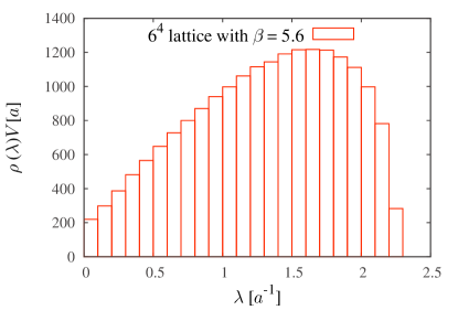
Figure 1: The Dirac spectral density $\rho(\lambda)$ on $6^{4}$ lattice with $\beta=5.6$, i.e., $a\simeq 0.25$ fm. Because of $\rho(-\lambda)=\rho(\lambda)$, only the positive region of $\lambda$ is shown. The bin-width is taken as $\Delta\lambda=0.1a^{-1}$. The total number of eigenmodes is $6^{4}\times 3=3888$.

Figure 2 is the scatter plot of the original (no Dirac-mode cut) Polyakov loop $\langle L_{P}\rangle$ for 50 gauge configurations. As shown in Fig. 2, $\langle L_{P}\rangle$ is almost zero, and $Z_{3}$-center symmetry is unbroken.

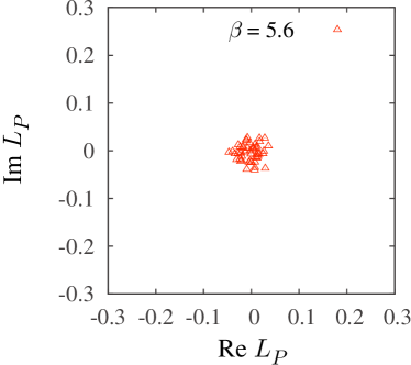
Figure 2: The scatter plot of the Polyakov loop $\langle L_{P}\rangle$ in the confined phase on the periodic lattice of $6^{4}$ and $\beta=5.6$, i.e., $a\simeq 0.25$ fm.

First, we analyze the role of low-lying Dirac-modes using the 50 gauge configurations. Figure 3 shows IR-cut spectral density

$$\rho_{\rm IR}(\lambda)\equiv\rho(\lambda)\theta(|\lambda|-\Lambda_{\rm IR}),$$ (27)

and the scatter plot of the IR-cut Polyakov loop $\langle L_{P}\rangle_{\rm IR}$ for $\Lambda_{\rm IR}=0.5a^{-1}$, which corresponds to about 400 modes removing from full eigenmodes. By this removal of low-lying Dirac modes below $\Lambda_{\rm IR}=0.5a^{-1}\simeq 0.4$ GeV, the IR-cut chiral condensate $\langle\bar{q}q\rangle_{\rm IR}$ is extremely reduced as

$${\langle\bar{q}q\rangle_{\rm IR}}/{\langle\bar{q}q\rangle}\simeq 0.02$$ (28)

around the physical region of the current quark mass, $m\simeq 0.006a^{-1}\simeq 5$ MeV Gongyo:2012 .

As shown in Fig. 3(b), even without the low-lying Dirac-modes, the IR-cut Polyakov loop is still almost zero Gongyo:2012 ,

$$\langle L_{P}\rangle_{\rm IR}\simeq 0$$ (29)

and $Z_{3}$-center symmetry is unbroken. This result shows that the single-quark energy remains extremely large, and the system is still in the confined phase even without low-lying Dirac-modes.

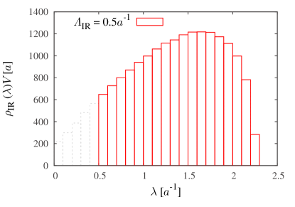
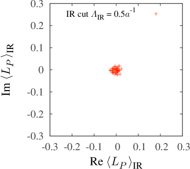
Figure 3: (a) The IR-cut Dirac spectral density $\rho_{\rm IR}(\lambda)\equiv\rho(\lambda)\theta(|\lambda|-\Lambda_{\rm IR})$ and (b) the IR-cut Polyakov loop $\langle L_{P}\rangle_{\rm IR}$ on the periodic lattice of $6^{4}$ at $\beta=5.6$ for the IR-cut of $\Lambda_{\rm IR}=0.5a^{-1}$.

Second, we consider the high Dirac-mode contribution to the Polyakov loop in the confined phase below $T_{c}$. In this case, the chiral condensate is almost unchanged. Figure 4 shows the UV-cut spectral density

$$\rho_{\rm UV}(\lambda)\equiv\rho(\lambda)\theta(\Lambda_{\rm UV}-|\lambda|),$$ (30)

and the UV-cut Polyakov loop $\langle L_{P}\rangle_{\rm UV}$ for $\Lambda_{\rm UV}=2.0a^{-1}$, corresponding to the removal of about 400 modes. Similar to the cut of low-lying modes, the UV-cut Polyakov loop is almost zero as $\langle L_{P}\rangle_{\rm UV}\simeq 0$, and indicates the confinement.

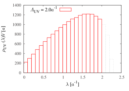
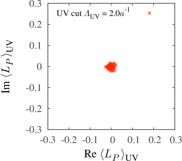
Figure 4: (a) The UV-cut Dirac spectral density $\rho_{\rm UV}(\lambda)\equiv\rho(\lambda)\theta(\Lambda_{\rm UV}-|\lambda|)$ and (b) the UV-cut Polyakov loop $\langle L_{P}\rangle_{\rm UV}$ on the periodic lattice of $6^{4}$ at $\beta=5.6$ for $\Lambda_{\rm UV}=2.0a^{-1}$.

Thus, in both cuts of low-lying Dirac modes in Fig. 3(b) and high modes in Fig. 4(b), the Polyakov loop $\langle L_{P}\rangle_{\rm IR/UV}$ is almost zero, which means that the system remains in the confined phase. In fact, we find “Dirac-mode insensitivity” to the Polyakov loop or the confinement property. We also examine the removal of intermediate (IM) Dirac-modes from the Polyakov loop in the confined phase in Appendix A, and find the similar Dirac-mode insensitivity. It suggests that each eigenmode has the information of confinement, and the Polyakov loop is not affected by removing of any eigenvalue region. Therefore, we consider that there is no direct correspondence between the Dirac eigenmodes and the Polyakov loop in the confined phase. This Dirac-mode insensitivity to confinement is consistent with the previous Wilson-loop analysis Suganuma:2011 ; Gongyo:2012 .

3.2 Dirac-mode projected Polyakov loop in the deconfined phase

Next, we investigate the Polyakov loop in the deconfined phase at high temperature. Here, we use periodic lattice of $6^{3}\times 4$ at $\beta=6.0$, which corresponds to $a\simeq 0.10$ fm and $T\equiv 1/(N_{t}a)\simeq 0.5$ GeV.

As shown in Fig. 5, the Polyakov loop has non-zero expectation values as $\langle L_{P}\rangle\neq 0$, and shows $Z_{3}$-center group structure on the complex plane. This behavior means the deconfined and center-symmetry broken phase.

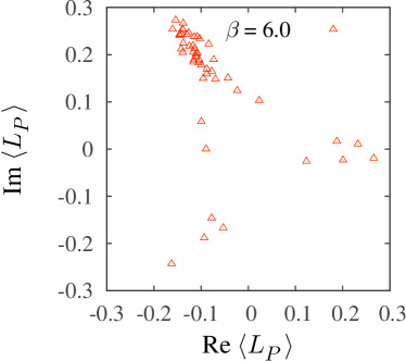
Figure 5: The scatter plot of the Polyakov loop $L_{P}$ in the deconfined phase on the periodic lattice of $6^{3}\times 4$ at $\beta=6.0$, corresponding to $a\simeq 0.10$ fm and $T\equiv 1/(N_{t}a)\simeq 0.5$ GeV.

To begin with, we investigate the difference of the Dirac spectral density $\rho(\lambda)$ between the confined and the deconfined phases. Figure 6 shows the Dirac spectral density in the deconfined phase at high temperature on $6^{3}\times 4$ at $\beta=6.0$, i.e., $T\simeq 0.5$ GeV. For comparison, we also add the spectrum density in the confined phase at low temperature on $6^{3}\times 4$ at $\beta=5.6$, i.e., $a\simeq 0.25$ fm and $T=1/(N_{t}a)\simeq 0.2$ GeV, below the critical temperature $T_{c}\simeq 0.26$ GeV at the quenched level. In both phases, the total number of eigenmodes is $6^{3}\times 4\times 3=2592$. As shown in Fig. 6, the low-lying Dirac eigenmodes are suppressed in the high-temperature phase, which leads to the chiral restoration.

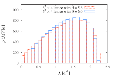
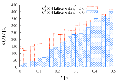
Figure 6: The Dirac spectrum density $\rho(\lambda)$ in confined phase ($\beta=5.6$) and deconfined phase ($\beta=6.0$) on $6^{3}\times 4$ lattice. (a) The comparison on full spectral densities. (b) The comparison on low-lying spectral densities.

We show the Dirac-mode projected Polyakov loop $\langle L_{P}\rangle_{\rm IR/UV}$ at $\Lambda_{\rm IR}=0.5a^{-1}$ and $\Lambda_{\rm UV}=2.0a^{-1}$ in Figs. 7(a) and (b), respectively. These mode-cuts correspond to removing about 200 modes from full eigenmodes. According to the removal of about 200 modes, there appears a trivial reduction (or normalization) factor for the IR/UV-cut Polyakov loop $\langle L_{P}\rangle_{\rm IR/UV}$.

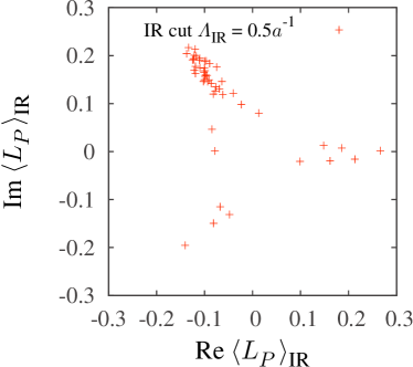
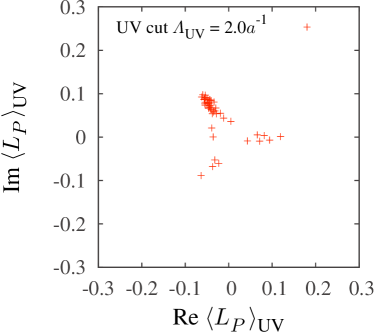
Figure 7: The scatter plot of the IR/UV-cut Polyakov loop in the deconfined phase on the periodic lattice of $6^{3}\times 4$ at $\beta=6.0$, i.e., $a\simeq 0.10$ fm and $T\equiv 1/(N_{t}a)\simeq 0.5$ GeV. (a) $\langle L_{P}\rangle_{\rm IR}$ in the case of IR Dirac-mode cut of $\Lambda_{\rm IR}=0.5a^{-1}$. (b) $\langle L_{P}\rangle_{\rm UV}$ in the case of UV Dirac-mode cut of $\Lambda_{\rm UV}=2.0a^{-1}$. According to the mode cut, there appears a constant reduction factor.

As shown in Fig. 7, both IR/UV-cut Polyakov loops $\langle L_{P}\rangle_{\rm IR/UV}$ are non-zero and show the characteristic $Z_{3}$ structure, similar to the original Polyakov loop $\langle L_{P}\rangle$. This suggests Dirac-mode insensitivity also in the deconfined phase. In Appendix A, we show the IM-cut Polyakov loop $\langle L_{P}\rangle_{\rm IM}$ in the deconfined phase, and find the similar results.

We also note that the absolute value of UV-cut Polyakov loop $\langle L_{P}\rangle_{\rm UV}$ is smaller than that of IR-cut one $\langle L_{P}\rangle_{\rm IR}$ in each gauge configuration, as shown in Fig. 7, in spite of almost the same number of removed IR/UV-modes. In fact, as the quantitative effect to the Polyakov loop, the contribution of UV Dirac-modes is larger than that of IR Dirac-modes Bruckmann:2007 , although the deconfinement nature indicated by the non-zero Polyakov loop does not change by the removal of IR or UV Dirac-modes.

Thus, the Polyakov-loop behavior and the $Z_{3}$ center symmetry are rather insensitive to the removal of the Dirac-modes in the IR, IM or UV region in both confined and deconfined phases. Therefore, we conclude that there is no clear correspondence between the Dirac-modes and the Polyakov loop in both confined and deconfined phases.

3.3 Temperature dependence of the Dirac-mode projected Polyakov loop

So far, we have analyzed the role of the Dirac-mode to the Polyakov loop in both confined and deconfined phases. In this subsection, we consider the temperature dependence of the Polyakov loop in terms of the Dirac-mode by varying the lattice parameter $\beta$ at fixed $N_{t}$. Here, we use $6^{3}\times 4$ lattice with $\beta=5.4\sim 6.0$.

Now, we investigate the gauge-configuration average of the absolute value of the IR/UV-cut Polyakov loop,

$$\langle|L_{P}^{\rm IR/UV}|\rangle\equiv\frac{1}{N_{\rm conf}}\sum_{k=1}^{N_{\rm conf}}|\langle L_{P}\rangle^{\rm IR/UV}_{k}|,$$ (31)

where $\langle L_{P}\rangle^{\rm IR/UV}_{k}$ denotes the IR/UV-cut Polyakov loop obtained from $k$-th gauge configuration, and $N_{\rm conf}$ the gauge configuration number.

Figure 8 shows $\beta$-dependence of the absolute value of the IR-cut Polyakov loop $\langle|L_{P}^{\rm IR}|\rangle$ with the low-lying cut ($\Lambda_{\rm IR}=0.5a^{-1},1.0a^{-1}$), and the UV-cut Polyakov loop $\langle|L_{P}^{\rm UV}|\rangle$ with the UV cut ($\Lambda_{\rm UV}=2.0a^{-1},1.7a^{-1}$). The numbers of the removed Dirac modes for $\Lambda_{\rm IR}=0.5a^{-1}$ and $1.0a^{-1}$ are approximately equal to $\Lambda_{\rm UV}=2.0a^{-1}$ and $1.7a^{-1}$, respectively. For comparison, we also add the original Polyakov loop $\langle|L_{P}|\rangle$, which shows the deconfinement phase transition around $\beta=5.6\sim 5.7$.

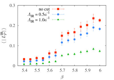
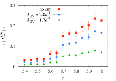
Figure 8: The $\beta$-dependence of the IR/UV-cut Polyakov loop $\langle|L_{P}^{\rm IR/UV}|\rangle$ on $6^{3}\times 4$ lattice. (a) $\langle|L_{P}^{\rm IR}|\rangle$ for the IR Dirac-mode cut of $\Lambda_{\rm IR}=0.5a^{-1}$ and $1.0a^{-1}$. (b) $\langle|L_{P}^{\rm UV}|\rangle$ for the UV-cut of $\Lambda_{\rm UV}=2.0a^{-1}$ and $1.7a^{-1}$. According to the mode cut, there appears a reduction factor for $\langle L_{P}\rangle_{\rm IR/UV}$.

As shown in Fig. 8, both IR-cut and UV-cut Polyakov loops $\langle|L_{P}^{\rm IR/UV}|\rangle$ show almost the same $\beta$-dependence of the original one $\langle|L_{P}|\rangle$, apart from a normalization factor. Thus, we find again no direct connection between the Polyakov-loop properties and the Dirac-eigenmodes. This result is consistent with the similar analysis for the Wilson loop using the Dirac-mode expansion method. Even after removing IR/UV Dirac-modes, the Wilson loop $\langle W\rangle_{\rm IR/UV}$ exhibits the area law with the same slope, i.e., the confining force $\sigma$ Suganuma:2011 ; Gongyo:2012 .

We also show the $\beta$-dependence of the chiral condensate $\langle\bar{q}q\rangle$ in the case of removing IR and UV Dirac modes, respectively. Note that, once the Dirac eigenvalues $\lambda_{n}$ are obtained, the chiral condensate can be easily calculated. In fact, the chiral condensate is expressed as

$$\langle\bar{q}q\rangle = -\frac{1}{V}\mathrm{Tr}\frac{1}{{\ooalign{\hfil/\hfil\crcr$D$}}+m}=-\frac{1}{V}\sum_{n}\frac{1}{i\lambda_{n}+m}$$ (34)

$$= -\frac{1}{V}\left(\sum_{\lambda_{n}>0}\frac{2m}{\lambda_{n}^{2}+m^{2}}-\frac{\nu}{m^{2}}\right),$$ (35)

with the total number $\nu$ of the Dirac zero-modes. Then, the IR/UV-cut chiral condensate is expressed as

$$\langle\bar{q}q\rangle_{{\rm IR}} = -\frac{1}{V}\sum_{\lambda\geq\Lambda_{\rm IR}}\frac{2m}{\lambda^{2}+m^{2}},$$

$$\langle\bar{q}q\rangle_{{\rm UV}} = -\frac{1}{V}\sum_{0<\lambda\leq\Lambda_{\rm UV}}\frac{2m}{\lambda^{2}+m^{2}},$$ (36)

with the Dirac-mode cut $\Lambda_{\rm IR/UV}$, apart from the zero-mode contribution.

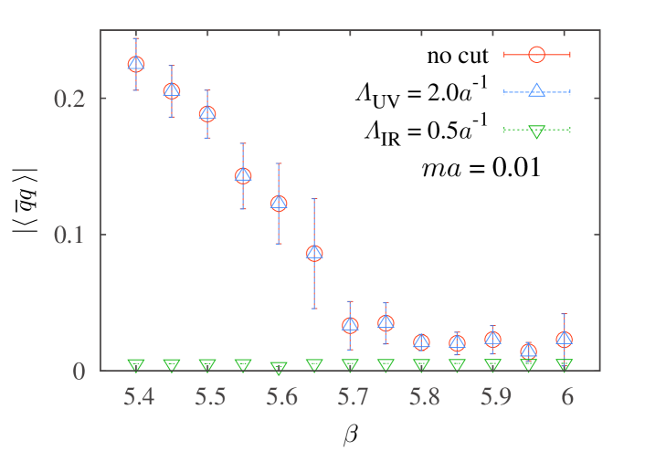
Figure 9: The $\beta$-dependence of the chiral condensate $\langle\bar{q}q\rangle_{{\rm IR}/{\rm UV}}$ after removing IR/UV Dirac-modes on $6^{4}\times 4$ lattice. For comparison, we add the original (no Dirac-mode cut) condensate $\langle\bar{q}q\rangle$, which almost coincides with $\langle\bar{q}q\rangle_{{\rm UV}}$.

Figure 9 shows the IR-cut chiral condensate $\langle\bar{q}q\rangle_{\rm IR}$ with $\Lambda_{\rm IR}=0.5a^{-1}$, and the UV-cut chiral condensate $\langle\bar{q}q\rangle_{\rm UV}$ with $\Lambda_{\rm UV}=2.0a^{-1}$, as a function of $\beta$. Here, the current quark mass is taken as $m=0.01a^{-1}$. For comparison, we also add the original (no Dirac-mode cut) chiral condensate $\langle\bar{q}q\rangle$. The chiral phase transition occurs around $\beta=5.6\sim 5.7$, which coincides with the deconfinement transition indicated by the Polyakov loop in Fig. 8. The chiral condensate is almost unchanged by the UV-mode cut as $\langle\bar{q}q\rangle_{\rm UV}\simeq\langle\bar{q}q\rangle$. On the other hand, the chiral condensate is drastically changed and becomes almost zero as $\langle\bar{q}q\rangle_{\rm IR}\simeq 0$ by the IR Dirac-mode cut in the whole region of $\beta$. This clearly shows the essential role of the low-lying Dirac-modes to the chiral condensate. However, the Polyakov-loop behavior is insensitive to the Dirac-mode, as shown in Fig. 8.

4 A new method to remove low-lying Dirac-modes from Polyakov loop for large lattices

In this section, as a convenient formalism, we propose a new method to remove low-lying Dirac-modes from the Polyakov loop without evaluating full Dirac-modes. Here, we consider the removal of a small number of low-lying Dirac modes, since only these modes are responsible to chiral symmetry breaking. For the Polyakov loop, unlike the Wilson loop, we can easily perform its practical calculation after removing the low-lying Dirac modes, by the reformulation with respect to the removed IR Dirac-mode space, which enables us to calculate with larger lattices.

As a numerical problem, it costs huge computational power to obtain the full eigenmodes of the large matrix / $D$ , and thus our analysis was restricted to relatively small lattices in the previous section. However, in usual eigenvalue problems, e.g., in the quantum mechanics, one often needs only a small number of low-lying eigenmodes. and there are several useful algorithms such as the Lanczos method to evaluate only low-lying eigenmodes, without performing full diagonalization of the matrix.

4.1 Reformulation of IR Dirac mode subtraction

The basic idea is to use only the low-lying Dirac modes. In fact, we calculate only the low-lying Dirac eigenfunction $\psi_{n}(x)\equiv\langle x|n\rangle$ for $|\lambda_{n}|<\Lambda_{\rm IR}$, and the IR matrix elements

$$\langle n|\hat{U}_{\mu}|m\rangle=\sum_{x}\psi_{n}^{\dagger}(x)U_{\mu}(x)\psi_{m}(x+\hat{\mu})$$ (37)

for $|\lambda_{n}|,|\lambda_{m}|<\Lambda_{\rm IR}$. We reformulate the Dirac-mode projection only with the small number of the low-lying Dirac modes of $|\lambda_{n}|<\Lambda_{\rm IR}$.

Here, the IR mode-cut operator $\hat{P}_{\rm IR}$ is expressed as

$$\hat{P}_{\rm IR} \equiv \sum_{|\lambda_{n}|\geq\Lambda_{\rm IR}}|n\rangle\langle n|=1-\sum_{|\lambda_{n}|<\Lambda_{\rm IR}}|n\rangle\langle n|=1-\hat{Q},$$ (38)

with the IR Dirac-mode projection operator

$$\hat{Q}\equiv\sum_{|\lambda_{n}|<\Lambda_{\rm IR}}|n\rangle\langle n|,$$ (39)

corresponding to the low-lying Dirac modes to be removed. Note that $\sum_{|\lambda_{n}|<\Lambda_{\rm IR}}$ in $\hat{Q}$ is the sum over only the low-lying modes, of which number is small, so that this sum is practically performed even for larger lattices. Then, we reformulate the Dirac-mode projection with respect to $\hat{Q}$ or the small-number sum of $\sum_{|\lambda_{n}|<\Lambda_{\rm IR}}$.

We rewrite the IR Dirac-mode cut Polyakov loop as

$$\langle L_{P}\rangle_{\rm IR} = \frac{1}{3V}\mathrm{Tr}\{(\hat{U}_{4}^{P})^{N_{t}}\}=\frac{1}{3V}\mathrm{Tr}\{(\hat{U}_{4}\hat{P})^{N_{t}}\}=\frac{1}{3V}\mathrm{Tr}[\{\hat{U}_{4}(1-\hat{Q})\}^{N_{t}}],$$ (40)

and expand $\langle L_{P}\rangle_{\rm IR}$ in terms of $\hat{Q}$.

As a simple example of the $N_{t}=2$ case, the IR-cut Polyakov loop $\langle L_{P}\rangle_{\rm IR}$ is written as

$$3V\langle L_{P}\rangle_{\rm IR} = \mathrm{Tr}\{\hat{U}_{4}(1-\hat{Q})\hat{U}_{4}(1-\hat{Q})\}$$ (41)

$$= \mathrm{Tr}(\hat{U}_{4}^{2})-2\mathrm{Tr}(\hat{Q}\hat{U}_{4}^{2})+\mathrm{Tr}(\hat{Q}\hat{U}_{4}\hat{Q}\hat{U}_{4})$$

$$= 3V\langle L_{P}\rangle-2\sum_{|\lambda_{n}|<\Lambda_{\rm IR}}\langle n|\hat{U}_{4}^{2}|n\rangle+\sum_{|\lambda_{n}|,|\lambda_{m}|<\Lambda_{\rm IR}}\langle n|\hat{U}_{4}|m\rangle\langle m|\hat{U}_{4}|n\rangle,$$

where $\langle L_{P}\rangle$ is the ordinary (no cut) Polyakov loop, and is easily obtained. In Eq. (41), we only need the IR matrix elements $\langle n|\hat{U}_{4}|m\rangle$ and

$$\langle n|\hat{U}_{4}^{2}|m\rangle \equiv \sum_{x}\sum_{y}\sum_{z}\langle n|x\rangle\langle x|\hat{U}_{4}|y\rangle\langle y|\hat{U}_{4}|z\rangle\langle z|m\rangle$$ (42)

$$= \sum_{x}\psi_{n}^{\dagger}(x)U_{4}(x)U_{4}(x+\hat{t})\psi_{m}(x+2\hat{t})\quad\qquad$$

for $|\lambda_{n}|,|\lambda_{m}|<\Lambda_{\rm IR}$. Here, $\hat{t}$ denotes the temporal unit vector in the lattice unit. In this way, using Eq. (41), we can remove the contribution of the low-lying Dirac-modes from the Polyakov loop, only with the IR matrix elements.

For the $N_{t}=4$ case, the IR-cut Polyakov loop $\langle L_{P}\rangle_{\rm IR}$ is expressed as

$$3V\langle L_{P}\rangle_{\rm IR} = \mathrm{Tr}\{(\hat{U}_{4}^{P})^{4}\}$$ (43)

$$= \mathrm{Tr}\{\hat{U}_{4}(1-\hat{Q})\hat{U}_{4}(1-\hat{Q})\hat{U}_{4}(1-\hat{Q})\hat{U}_{4}(1-\hat{Q})\}$$

$$= \mathrm{Tr}(\hat{U}_{4}^{4})-4\mathrm{Tr}(\hat{Q}\hat{U}_{4}^{4})+4\mathrm{Tr}(\hat{Q}\hat{U}_{4}\hat{Q}\hat{U}_{4}^{3})$$

$$\quad+2\mathrm{Tr}(\hat{Q}\hat{U}_{4}^{2}\hat{Q}\hat{U}_{4}^{2})-4\mathrm{Tr}(\hat{Q}\hat{U}_{4}\hat{Q}\hat{U}_{4}\hat{Q}\hat{U}_{4}^{2})+\mathrm{Tr}(\hat{Q}\hat{U}_{4}\hat{Q}\hat{U}_{4}\hat{Q}\hat{U}_{4}\hat{Q}\hat{U}_{4})$$

$$= 3V\left\{\langle L_{P}\rangle-L_{P}^{(1)}+L_{P}^{(2)}-L_{P}^{(3)}+L_{P}^{(4)}\right\},$$

where $L_{P}^{(i)}$ ($i=1,2,3,4$) are the IR Dirac-mode contributions expanded in terms of $\hat{Q}$, and are given by

$$L_{P}^{(1)}\equiv\frac{4}{3V}\mathrm{Tr}(\hat{Q}\hat{U}_{4}^{4})=\frac{4}{3V}\sum_{n_{1}}^{\rm IR}\langle n_{1}|\hat{U}_{4}^{4}|n_{1}\rangle,$$ (44)

$$L_{P}^{(2)} \equiv \frac{4}{3V}\mathrm{Tr}(\hat{Q}\hat{U}_{4}\hat{Q}\hat{U}_{4}^{3})+\frac{2}{3V}\mathrm{Tr}(\hat{Q}\hat{U}_{4}^{2}\hat{Q}\hat{U}_{4}^{2})$$ (45)

$$= \frac{4}{3V}\sum_{n_{1},n_{2}}^{\rm IR}\langle n_{1}|\hat{U}_{4}|n_{2}\rangle\langle n_{2}|\hat{U}_{4}^{3}|n_{1}\rangle+\frac{2}{3V}\sum_{n_{1},n_{2}}^{\rm IR}\langle n_{1}|\hat{U}_{4}^{2}|n_{2}\rangle\langle n_{2}|\hat{U}_{4}^{2}|n_{1}\rangle,$$

$$L_{P}^{(3)} \equiv \frac{4}{3V}\mathrm{Tr}(\hat{Q}\hat{U}_{4}\hat{Q}\hat{U}_{4}\hat{Q}\hat{U}_{4}^{2})=\sum_{n_{1},n_{2},n_{3}}^{\rm IR}\langle n_{1}|\hat{U}_{4}|n_{2}\rangle\langle n_{2}|\hat{U}_{4}|n_{3}\rangle\langle n_{3}|\hat{U}_{4}^{2}|n_{1}\rangle,$$ (46)

$$L_{P}^{(4)} \equiv \frac{1}{3V}\mathrm{Tr}(\hat{Q}\hat{U}_{4}\hat{Q}\hat{U}_{4}\hat{Q}\hat{U}_{4}\hat{Q}\hat{U}_{4})$$ (47)

$$= \frac{1}{3V}\sum_{n_{1},n_{2},n_{3},n_{4}}^{\rm IR}\langle n_{1}|\hat{U}_{4}|n_{2}\rangle\langle n_{2}|\hat{U}_{4}|n_{3}\rangle\langle n_{3}|\hat{U}_{4}|n_{4}\rangle\langle n_{4}|\hat{U}_{4}|n_{1}\rangle.$$

Here, the summation $\sum^{\rm IR}$ is taken over only low-lying Dirac modes with $|\lambda_{n}|<\Lambda_{\rm IR}$, of which number is small. In Eq. (43), we only need the IR matrix elements $\langle n|\hat{U}_{4}^{k}|m\rangle$ ($k$=1,2,3,4) for $|\lambda_{n}|,|\lambda_{m}|<\Lambda_{\rm IR}$, and they can be calculated as

$$\langle n|\hat{U}_{4}^{k}|m\rangle = \sum_{x}\langle n|x\rangle\langle x|\hat{U}_{4}|x+\hat{t}\rangle\langle x+\hat{t}|\hat{U}_{4}|x+2\hat{t}\rangle\cdots\langle x+(k-1)\hat{t}|\hat{U}_{4}|x+k\hat{t}\rangle\langle x+k\hat{t}|m\rangle$$ (48)

$$= \sum_{x}\psi_{n}^{\dagger}(x)U_{4}(x)U_{4}(x+\hat{t})\cdots U_{4}(x+(k-1)\hat{t})\psi_{m}(x+k\hat{t}).$$

In particular of $k=N_{t}$, this matrix element is simplified as

$$\langle n|\hat{U}_{4}^{N_{t}}|m\rangle=\sum_{x}\psi_{n}^{\dagger}(x)U_{4}(x)\cdots U_{4}(x+(N_{t}-1)\hat{t})\psi_{m}(x)=\sum_{x}\psi_{n}^{\dagger}(x)L_{P}(x)\psi_{m}(x),$$ (49)

with the ordinary Polyakov-loop operator $L_{P}(x)$.

Thus, using Eqs. (43) and (48), we can perform the actual calculation of the IR Dirac-mode cut Polyakov loop $\langle L_{P}\rangle_{\rm IR}$, only with the IR matrix elements on the low-lying Dirac modes. In this method, we need not full diagonalization of the Dirac operator, and hence the calculation cost is extremely reduced.

In principle, we can generalize this method for larger temporal-size lattice and the Wilson-loop analysis, although the number of the terms becomes larger in these cases.

4.2 Lattice QCD analysis of IR Dirac-mode contribution to Polyakov loop

Before applying this method to larger-volume lattice calculations, we investigate the IR Dirac-mode contribution to the Polyakov loop, $L_{P}^{(i)}$ defined in Eqs. (44)$\sim$(47), on the periodic lattice of $6^{3}\times 4$ at $\beta=6.0$, which corresponds to the deconfined phase.

Here, $L_{P}^{(i)}$ ($i=1,2,3,4$) are the IR Dirac-mode contributions expanded in terms of the number of IR projection $\hat{Q}$, and satisfy

$$\langle L_{P}\rangle_{\rm IR}=\langle L_{P}\rangle-L_{P}^{(1)}+L_{P}^{(2)}-L_{P}^{(3)}+L_{P}^{(4)}.$$ (50)

In this expansion, one can identify $\langle L_{P}\rangle=L_{P}^{(0)}$, since the original Polyakov loop $\langle L_{P}\rangle$ includes no IR projection $\hat{Q}$.

We show in Fig. 10 the scatter plot of $L_{P}^{(1)}$, $L_{P}^{(2)}$, $L_{P}^{(3)}$, and $L_{P}^{(4)}$, together with $\langle L_{P}\rangle$, in the case of IR-cut of $\Lambda_{\rm IR}=0.5a^{-1}$. As shown in Fig. 10, all of the IR contributions $L_{P}^{(i)}$ ($i=1,2,3,4$) are rather small in comparison with $\langle L_{P}\rangle$. For each gauge configuration, we find

$$|\langle L_{P}\rangle|\gg|L_{P}^{(1)}|\gg|L_{P}^{(2)}|\gg|L_{P}^{(3)}|\gg|L_{P}^{(4)}|,$$ (51)

which leads to $\langle L_{P}\rangle_{\rm IR}\simeq\langle L_{P}\rangle$. Among the IR contribution, $L_{P}^{(1)}$ gives the dominant contribution, and higher order terms are almost negligible. Note also that each $L_{P}^{(i)}$ distributes in the $Z_{3}$-center direction on the complex plane, and $L_{P}^{(i)}$ in Eq. (50) partially cancels between odd $i$ and even $i$. In this way, the approximate magnitude and the $Z_{3}$ structure of the Polyakov loop would be unchanged by the IR Dirac-mode cut.

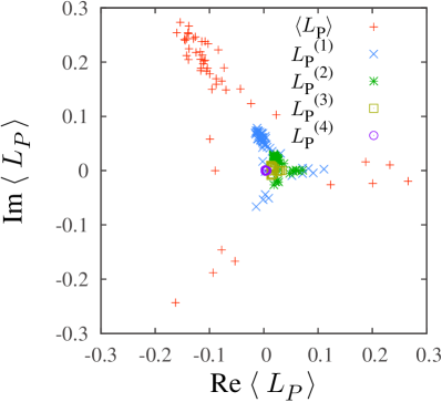
Figure 10: IR Dirac-mode contributions to the Polyakov loop, $L_{P}^{(1)}$, $L_{P}^{(2)}$, $L_{P}^{(3)}$, and $L_{P}^{(4)}$ defined in Eqs. (44)$\sim$(47), in the case of $\Lambda_{\rm IR}=0.5a^{-1}$, in the deconfined phase on the periodic lattice of $6^{3}\times 4$ at $\beta=6.0$. For comparison, the original Polyakov loop $\langle L_{P}\rangle$ is added.

4.3 Lattice QCD result for a larger-volume lattice

Now, we show the lattice QCD result for the Polyakov loop after removing low-lying Dirac modes from the confined phase on a larger periodic lattice. Figure 11 shows the scatter plot of the IR-cut Polyakov loop $\langle L_{P}\rangle_{\rm IR}$ on the quenched lattice of $12^{3}\times 4$ at $\beta=5.6$, i.e., $a\simeq$ 0.25 fm and $T=1/(N_{t}a)\simeq 0.2$ GeV below $T_{c}\simeq 0.26$ GeV, using 50 gauge configurations. For comparison, the original (no-cut) Polyakov loop $\langle L_{P}\rangle$ is also shown in Fig. 11. Here, we use ARPACK ARPACK to calculate low-lying Dirac eigenmodes. On the IR-cut parameter, we use $\Lambda_{\rm IR}=0.08a^{-1}$, which corresponds to the removal of about 180 low-lying Dirac modes from the total 20736 modes. In this case, the IR-cut quark condensate $\langle\bar{q}q\rangle_{\rm IR}$ is reduced to be only about 7%, i.e., $\langle\bar{q}q\rangle_{\rm IR}/\langle\bar{q}q\rangle\simeq 0.07$, around the physical current-quark mass of $m\simeq 0.006a^{-1}\simeq$ 5 MeV.

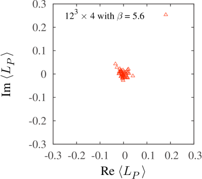
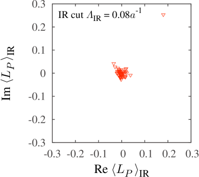
Figure 11: The Polyakov loop $\langle L_{P}\rangle$ (upper) and the IR Dirac-mode cut Polyakov loop $\langle L_{P}\rangle_{\rm IR}$ (lower) with $\Lambda_{\rm IR}\simeq 0.08a^{-1}$ on $12^{3}\times 4$ lattice at $\beta=5.6$ (confinement phase).

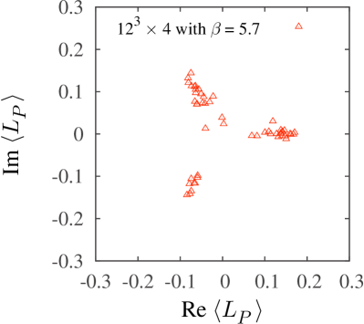
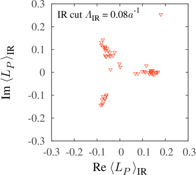
Figure 12: The Polyakov loop $\langle L_{P}\rangle$ (upper) and the IR Dirac-mode cut Polyakov loop $\langle L_{P}\rangle_{\rm IR}$ (lower) with $\Lambda_{\rm IR}\simeq 0.08a^{-1}$ on $12^{3}\times 4$ lattice at $\beta=5.7$ (deconfinement phase).

Note again that the IR-cut Polyakov loop is almost zero as $\langle L_{P}\rangle_{\rm IR}\simeq 0$ and the $Z_{3}$ center symmetry is kept, that is, the confinement is still realized, even without the low-lying Dirac modes, which are essential for chiral symmetry breaking.

Next, we show the removal of low-lying Dirac modes from the deconfined phase on a larger periodic lattice. Figure 12 shows the IR-cut Polyakov loop $\langle L_{P}\rangle_{\rm IR}$ together with $\langle L_{P}\rangle$ on $12^{3}\times 4$ at $\beta=5.7$, i.e., $a\simeq$ 0.186 fm Takahashi and $T\equiv 1/(N_{t}a)\simeq$ 0.27 GeV above $T_{c}$, using 50 gauge configurations. We use $\Lambda_{\rm IR}=0.08a^{-1}$, which corresponds to the removal of about 120 low-lying Dirac modes from the total 20736 modes. In this case, we find $\langle L_{P}\rangle_{\rm IR}\simeq\langle L_{P}\rangle$ for each gauge configuration, and observe almost no effect of the IR Dirac-mode removal for the Polyakov loop.

Thus, for both confined and deconfined phases, the Polyakov-loop behavior is almost unchanged by removing the low-lying Dirac modes, in terms of the zero/non-zero expectation value and the $Z_{3}$ center symmetry. In fact, we find again the IR Dirac-mode insensitivity to the Polyakov-loop or the confinement property also for the larger volume lattice.

5 Summary and Concluding Remarks

In this paper, we have investigated the direct correspondence between the Polyakov loop and the Dirac eigenmodes in a gauge-invariant manner in SU(3) lattice QCD at the quenched level in both confined and deconfined phases. Based on the Dirac-mode expansion method, we have removed the essential ingredient of chiral symmetry breaking from the Polyakov loop.

In the confined phase, we have found that the IR-cut Polyakov loop $\langle L_{P}\rangle_{\rm IR}$ is still almost zero even without low-lying Dirac eigenmodes. As shown in the Banks-Casher relation, these low-lying modes are essential for chiral symmetry breaking. This result indicates that the system still remains in the confined phase after the effective restoration of chiral symmetry. We have also analyzed the role of high (UV) Dirac-modes, and have found that the UV-cut Polyakov loop $\langle L_{P}\rangle_{\rm UV}$ is also zero. These results indicate that there is no definite Dirac-modes region relevant for the Polyakov-loop behavior, in fact, each Dirac eigenmode seems to feel that the system is in the confined phase.

This Dirac-mode insensitivity to the confinement is consistent with the previous Wilson-loop analysis with the Dirac-mode expansion in Refs.Suganuma:2011 ; Gongyo:2012 , where the Wilson loop shows area law and linear confining potential is almost unchanged even without low-lying or high Dirac eigenmodes. These results are also consistent with the existence of hadrons as bound states without low-lying Dirac-modes Lang:2011 ; Glozman:2012 . Also, Gattringer’s formula suggests that the existence of Dirac zero-modes does not seem to contribute to the Polyakov loop Gattringer:2006 .

Next, we have analyzed the Polyakov loop in the deconfined phase at high temperature, where the Polyakov loop $\langle L_{P}\rangle$ has a non-zero expectation value, and its value distributes in $Z_{3}$ direction in the complex plane. We have found that both IR-cut and UV-cut Polyakov loops $\langle L_{P}\rangle_{\rm IR/UV}$ have the same properties of the non-zero expectation value and the $Z_{3}$ symmetry breaking.

We have also investigated the temperature dependence of the IR/UV-cut Polyakov loop $\langle L_{P}\rangle_{\rm IR/UV}$, and have found that $\langle L_{P}\rangle_{\rm IR/UV}$ shows almost the same temperature dependence as the original Polyakov loop $\langle L_{P}\rangle$, while the IR-cut chiral condensate $\langle\bar{q}q\rangle_{\rm IR}$ becomes almost zero even below $T_{c}$, after removing the low-lying Dirac-modes.

Finally, we have developed a new method to calculate the IR-cut Polyakov loop $\langle L_{P}\rangle_{\rm IR}$ in a larger volume at finite temperature, by the reformulation with respect to the removed IR Dirac-mode space, and have found again the IR Dirac-mode insensitivity to the Polyakov loop or the confinement property on a larger lattice of $12^{3}\times 4$.

These lattice QCD results and related studies Lang:2011 ; Glozman:2012 ; Suganuma:2011 ; Gongyo:2012 ; TMDoi suggest that each eigenmode has the information of confinement/deconfinement, i.e., the “seed” of confinement is distributed in a wider region of the Dirac eigenmodes. We consider that there is no direct connection between color confinement and chiral symmetry breaking through the Dirac eigenmodes. In fact, the one-to-one correspondence does not hold between confinement and chiral symmetry breaking in QCD, and their appearance can be different in QCD. This mismatch may suggest richer QCD phenomena and richer structures in QCD phase diagram. It is interesting to proceed full QCD and investigate dynamical quark effects in our framework. It is also interesting to search the relevant modes only for color confinement but irrelevant for chiral symmetry breaking Iritani:2012FP .

Appendix A Intermediate Dirac-mode removal for Polyakov loop

In this appendix, we study the role of the intermediate (IM) Dirac-modes to the Polyakov loop in both confined and deconfined phases. We consider the cut of IM Dirac modes of $\Lambda_{1}<|\lambda_{n}|<\Lambda_{2}$. Then, the IM-cut Polyakov-loop is defined as

$$\langle L_{P}\rangle_{\rm IM}\equiv\frac{1}{3V}\mathrm{tr}\sum_{|\lambda_{n_{i}}|\leq\Lambda_{\rm 1},\\ \Lambda_{\rm 2}\leq|\lambda_{n_{i}}|}\langle n_{1}|\hat{U}_{4}|n_{2}\rangle\cdots\langle n_{N_{t}}|\hat{U}_{4}|n_{1}\rangle,$$ (52)

with the cut parameters, $\Lambda_{1}$ and $\Lambda_{2}$.

Figures 13 and 14 show the IM-cut Polyakov loop $\langle L_{P}\rangle_{\rm IM}$ on the periodic lattice of $6^{4}$ at $\beta=5.6$ in the confined phase, and that of $6^{3}\times 4$ at $\beta=6.0$ in the deconfined phase, respectively. Here, we remove the IM modes of $0.5-1.0[a^{-1}]$, $1.0-1.5[a^{-1}]$, and $1.5-2.0[a^{-1}]$, respectively.

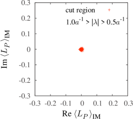
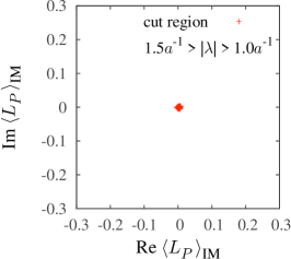
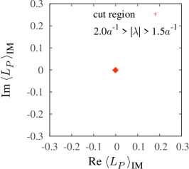
Figure 13: The IM-cut Polyakov loop on the periodic lattice of $6^{4}$ at $\beta=5.6$ in the confined phase. The cut region of the Dirac mode is (a) $|\lambda|\in(0.5a^{-1},1.0a^{-1})$, (b) $|\lambda|\in(1.0a^{-1},1.5a^{-1})$, and (c) $|\lambda|\in(1.5a^{-1},2.0a^{-1})$, respectively.

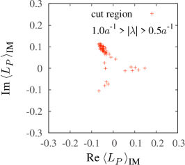
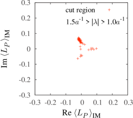
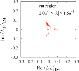
Figure 14: The IM-cut Polyakov loop on the periodic lattice of $6^{3}\times 4$ at $\beta=6.0$ in the deconfined phase. The cut region of the Dirac mode is (a) $|\lambda|\in(0.5a^{-1},1.0a^{-1})$, (b) $|\lambda|\in(1.0a^{-1},1.5a^{-1})$, and (c) $|\lambda|\in(1.5a^{-1},2.0a^{-1})$, respectively.

In the confined phase, the IM-cut Polyakov loop $\langle L_{P}\rangle_{\rm IM}$ is almost zero, and $\langle L_{P}\rangle_{\rm IM}$ has non-zero expectation value in the deconfined phase. These Dirac-mode insensitivities are similar to the case of IR/UV-cut Polyakov loops.

References

- (1) Y. Nambu and G. Jona-Lasinio, Phys. Rev. 122, 345 (1961); ibid. 124, 246 (1961).
- (2) H. Suganuma, S. Sasaki, and H. Toki, Nucl. Phys. B 435, 207 (1995); H. Suganuma, S. Sasaki, H. Toki, and H. Ichie, Prog. Theor. Phys. Suppl. 120, 57 (1995).
- (3) O. Miyamura, Phys. Lett. B353, 91 (1995).
- (4) R.M. Woloshyn, Phys. Rev. D51, 6411 (1995).
- (5) C. Gattringer, Phys. Rev. Lett. 97, 032003 (2006).
- (6) F. Bruckmann, C. Gattringer, and C. Hagen, Phys. Lett. B647, 56 (2007).
- (7) E. Bilgici and C. Gattringer, JHEP05, 030 (2008).
- (8) E. Bilgici, F. Bruckmann, C. Gattringer, and C. Hagen, Phys. Rev. D77, 094007 (2008).
- (9) F. Synatschke, A. Wipf, and K. Langfeld, Phys. Rev. D77, 114018 (2008).
- (10) J. Gattnar, C. Gattringer, K. Langfeld, H. Reinhardt, A. Schaefer, S. Solbrig, and T. Tok, Nucl. Phys. B716, 105 (2005).
- (11) R. Hollwieser, M. Faber, J. Greensite, U.M. Heller, and S. Olejnik, Phys. Rev. D78, 054508 (2008).
- (12) T.G. Kovacs, Phys. Rev. Lett. 104, 031601 (2010).
- (13) C.B. Lang and M. Schröck, Phys. Rev. D84, 087704 (2011); Proc. Sci., Lattice 2011 (2011) 111.
- (14) L.Ya. Glozman, C.B. Lang, and M. Schröck, Phys. Rev. D86, 014507 (2012).
- (15) H. Suganuma, S. Gongyo, T. Iritani, and A. Yamamoto, Proc. Sci., QCD-TNT-II (2011) 044; H. Suganuma, S. Gongyo, and T. Iritani, Proc. Sci., Lattice 2012 (2012) 217; Proc. Sci., Confinement X (2012) 081.
- (16) S. Gongyo, T. Iritani, and H. Suganuma, Phys. Rev. D86, 034510 (2012).
- (17) T. Iritani, S. Gongyo, and H. Suganuma, Proc. Sci., Lattice 2012 (2012) 212; Proc. Sci., Confinement X (2012) 053.
- (18) H. Suganuma, T.M. Doi, and T. Iritani, Proc. Sci., Lattice 2013 (2013) 374; Eur. Phys. J. Web of Conf. (ICNFP2013), arXiv:1312.6178 [hep-lat]; Proc. Sci., QCD-TNT-III (2014) 042; Proc. Sci., Hadron 2013 (2014) 121; T.M. Doi, H. Suganuma, and T. Iritani, Proc. Sci., Lattice 2013 (2013) 375; Proc. Sci., Hadron 2013 (2014) 122.
- (19) H.J. Rothe, Lattice Gauge Theories, (World Scientific, 2012), and its references.
- (20) F. Karsch, Nucl. Phys. A698, 199 (2002); Lect. Notes Phys. 583, 209 (2002), and references threin.
- (21) Y. Aoki, G. Endrodi, Z. Fodor, S. Katz, and K. Szabo, Nature 443, 675 (2006).
- (22) Y. Aoki, Z. Fodor, S.D. Katz, and K.K. Szabo, Phys. Lett. B643, 46 (2006).
- (23) Y. Aoki, S. Borsanyl, S. Durr, Z. Fodor, S.D. Katz, S. Krieg, and K.K. Szabo, JHEP06, 088 (2009).
- (24) F. Karsch and M. Lutgemeier, Nucl. Phys. B 550, 449 (1999).
- (25) J. Engels, S. Holtmann and T. Schulze, Nucl. Phys. B 724, 357 (2005).
- (26) G. Cossu, M. D’Elia, A. Di Giacomo, G. Lacagnina and C. Pica, Phys. Rev. D 77, 074506 (2008); G. Cossu and M. D’Elia, JHEP07, 048 (2009).
- (27) Y. Nambu, Phys. Rev. D10, 4262 (1974); G. ’t Hooft, in “High Energy Physics” (1975); S. Mandelstam, Phys. Rept. 23, 245 (1976).
- (28) G. ’t Hooft, Nucl. Phys. B190, 455 (1981).
- (29) A.S. Kronfeld, G. Schierholz, and U.-J. Wiese, Nucl. Phys. B293, 461 (1987); A.S. Kronfeld, M.L. Laursen, G. Schierholz, and U.-J. Wiese, Phys. Lett. B198, 516 (1987).
- (30) S. Hioki, S. Kitahara, S. Kiura, Y. Matsubara, O. Miyamura, S. Ohno, and T. Suzuki, Phys. Lett. B272, 326 (1991), Erratum-ibid. B281, 416 (1992).
- (31) J.D. Stack, S.D. Neiman, and R.J. Wensley, Phys. Rev. D50, 3399 (1994).
- (32) H. Suganuma, A. Tanaka, S. Sasaki, and O. Miyamura, Nucl. Phys. B (Proc. Suppl.) 47, 302 (1996).
- (33) K. Amemiya and H. Suganuma, Phys. Rev. D60, 114509 (1999); H. Suganuma, K. Amemiya, H. Ichie, and A. Tanaka, Nucl. Phys. A670, 40 (2000).
- (34) S. Gongyo, T. Iritani, and H. Suganuma, Phys. Rev. D86, 094018 (2012); S. Gongyo and H. Suganuma, Phys. Rev. D87, 074506 (2013).
- (35) T. Banks and A. Casher, Nucl. Phys. B169, 103 (1980).
- (36) F. Bruckmann and E.-M. Ilgenfritz, Phys. Rev. D72, 114502 (2005).
- (37) V. Gribov, Nucl. Phys. B193, 1 (1978).
- (38) D. Zwanziger, Phys. Rev. Lett.90, 102001 (2003).
- (39) J. Greensite and S. Olejník, Phys. Rev. D67, 094503 (2003); J. Greensite, Prog. Part. Nucl. Phys.51, 1 (2003).
- (40) J. Greensite, S. Olejník, and D. Zwanziger, Phys. Rev. D69, 074506 (2004).
- (41) J. Greensite, S. Olejník, and D. Zwanziger, JHEP05, 070 (2005).
- (42) M.F. Atiyah and I.M. Singer, Annals Math. 87, 484 (1968).
- (43) E. -M. Ilgenfritz, K. Koller, Y. Koma, G. Schierholz, T. Streuer, and V. Weinberg, Phys. Rev. D 76, 034506 (2007); E. -M. Ilgenfritz, D. Leinweber, P. Moran, K. Koller, G. Schierholz, and V. Weinberg, Phys. Rev. D 77, 074502 (2008), [Erratum-ibid. D 77, 099902 (2008)], and their references.
- (44) E. Anderson et al., LAPACK Users’ Guide (Society for Industrial and Applied Mathematics, Philadelphia, 1999).
- (45) L. Del Debbio, M. Faber, J. Greensite, and S. Olejník, Phys. Rev. D55, 2298 (1997); L. Del Debbio, M. Faber, J. Giedt, J. Greensite, and S. Olejník, Phys. Rev. D58, 094501 (1998).
- (46) Ph. de Forcrand and M. D’Elia, Phys. Rev. Lett. 82, 4582 (1999).
- (47) A. Yamamoto and H. Suganuma, Phys. Rev. Lett. 101, 241601 (2008); Phys. Rev. D79, 054504 (2009).
- (48) C. Gattringer, E. -M. Ilgenfritz and S. Solbrig, hep-lat/0601015, Proc. of “Sense of Beauty in Physics”, Pisa, Italy (2006).
- (49) T.T. Takahashi, H. Suganuma, Y. Nemoto, and H. Matsufuru, Phys. Rev. D65, 114509 (2002); T.T. Takahashi, H. Matsufuru, Y. Nemoto, and H. Suganuma, Phys. Rev. Lett. 86, 18 (2001).
- (50) R.B. Lehoucq, D.C. Sorensen, and C. Yang, ARPACK Users’ Guide (SIAM, New, York, 1998).
- (51) T. Iritani and H. Suganuma, Phys. Rev. D86, 074034 (2012).