Supernovae in the Central Parsec: A Mechanism for Producing Spatially Anisotropic Hypervelocity Stars

Abstract

Several tens of hyper-velocity stars (HVSs) have been discovered escaping our Galaxy. These stars share a common origin in the Galactic centre and are distributed anisotropically in Galactic longitude and latitude. We examine the possibility that HVSs may be created as the result of supernovae occurring within binary systems in a disc of stars around Sgr A^∗ over the last 100 Myr. Monte Carlo simulations show that the rate of binary disruption is $\sim 10^{-4}$ yr^-1, comparable to that of tidal disruption models. The supernova-induced HVS production rate ($\Gamma_{\rm HVS}$) is significantly increased if the binaries are hardened via migration through a gaseous disc. Moderate hardening gives $\Gamma_{\rm HVS}\simeq 2\times 10^{-7}$ yr^-1 and an estimated population of $\sim 20$ HVSs in the last $100$ Myr. Supernova-induced HVS production requires the internal and external orbital velocity vectors of the secondary binary component to be aligned when the binary is disrupted. This leaves an imprint of the disc geometry on the spatial distribution of the HVSs, producing a distinct anisotropy.

1. Introduction

In recent years, several tens of stars have been discovered moving through the Galaxy with large radial velocities (Brown et al., 2005, 2007). They are usually called ‘hypervelocity stars’ (HVSs), although the term is not precisely defined. Brown et al. (2012b) define HVS as a star with a Galactic rest-frame radial velocity $v_{\rm rf}>275$ km/s, with a sub-population of unbound HVSs having $v_{\rm rf}>400$ km/s.

Most HVSs are B-type stars with ages $t_{\rm HVS}\lesssim 200$ Myr (Brown et al., 2012a). The difference between the stellar age and the travel time from the Galactic centre (called the “arrival time”) has been determined for a few HVSs and lies between several tens - 100 Myr (Brown et al., 2012a).

The HVSs follow a statistically significant anisotropic distribution in galactic longitude and latitude and seem to form an extended, thick disc (Brown et al., 2009, 2012b). HVS velocities and orbits (e.g. Brown et al., 2005) strongly suggest an origin in the Galactic Centre (GC) close to Sgr A^∗. Few proper motion measurements of HVSs exist; two HVSs seem to originate in the Galactic disc (Heber et al., 2008; Tillich et al., 2009) and one seems to be confirmed as ejected from the GC (Brown et al., 2010, but see Irrgang et al. 2013 for a claim that the star’s origin in the LMC cannot be ruled out).

The dominant model explaining HVS ejection is the tidal disruption of binaries by Sgr A^∗, the supermassive black hole (SMBH) at the centre of our Galaxy. This model, and associated assumptions, can explain the production rates and velocities of the observed HVS population. An alternative model with a Galactic disc origin, the disruption of binary stars by supernova explosions, does not produce large enough velocities. We discuss HVS production mechanisms in more detail in Section 2 below. We note that there is another definition of HVS based on their production mechanism, with stars created via tidal disruption of binary stars (see below) termed HVSs and those produced by other channels termed ‘runaway’ or ‘hyper-runaway’ stars. In this Paper, we define HVSs only by their radial velocities.

In this paper we develop the idea that HVSs can be produced via supernova-induced disruption of binaries in the GC (Baruteau et al., 2011). We show this model to be consistent with the GC origin, anisotropic spatial distribution and arrival times of the observed HVS population. We propose that a disc of stars analogous to the discs of young stars currently observed in the central parsec (Paumard et al., 2006) formed during extended GC star formation over the last $\sim 10^{8}$ yr (Blum et al., 2003). Core-collapse supernovae will have disrupted many of these binaries, ejecting some secondary (less massive) stars with a range of terminal velocities. When the orbital velocities of binaries around Sgr A^∗ align with the internal orbital velocities of secondary stars within the binaries, the terminal velocity can reach as much as $>600$ km/s, potentially explaining most of the known HVSs. The original stellar disc provides a natural plane for the HVS spatial distribution. We find HVS production rates comparable to tidal disruption models and arrival times consistent with observation.

We begin by outlining the commonly investigated HVS production scenarios and highlight their major features in Section 2. The physical basis for the model and simulations is presented in Section 3. Section 4 presents the expected HVS production rates, spatial distribution and arrival times. We discuss the results in Section 5 and conclude in Section 6.

2. HVS production mechanisms

The earliest and most popular mechanism proposed for the ejection of HVSs is the tidal disruption of stellar binaries by the SMBH in the Galactic Center. In this scenario, originally proposed by Hills (1988) and later studied by Yu & Tremaine (2003), stellar binaries on low angular momentum orbits come close enough to the SMBH to be tidally disrupted in a three-body interaction. As a result, one star acquires a large velocity, possibly becoming an HVS, while the companion remains bound to the SMBH in a very eccentric orbit. Such bound stars may represent the progenitors of the S-stars (e.g. Gillessen et al., 2009; Perets et al., 2009). Models show that the S-stars and the HVSs can be produced from the same parent population (Zhang et al., 2013). Because of the large abundance of binaries in dense stellar environments, this process is considered a natural occurrence in galactic nuclei hosting supermassive black holes. The discovery of the first HVS star (Brown et al., 2005) helped to validate the scenario. The tidal disruption model predicts a continuous ejection of stars from the Galactic Center and an isotropic distribution of HVSs in the halo, unless the original stellar binaries are prevalently found in flattened systems like stellar disks (Lu et al., 2010). In the presence of a binary black hole, encounters with single stars also result in the acceleration of stars to hypervelocities, with a somewhat higher rate. Yu & Tremaine (2003) predict an ejection rate of the order of $10^{-5}$ yr^-1 for a single SMBH and $10^{-4}$ yr^-1 for a black hole binary, in agreement with available observations. However, production rates depend on several assumptions about the binary fraction in the Galactic Center, the state of the loss cone and the number of massive perturbers, such as giant molecular clouds or star clusters (Perets et al., 2007), and are uncertain within two or three orders of magnitude. Possible difficulties of the tidal disruption model include the observed anisotropic distribution of HVSs in the halo and the existence of HVSs with measured proper motion not originating from the Galactic Center (Heber et al., 2008; Tillich et al., 2009).

High velocity stars, generally called runaways, are produced in the Galactic disk by the disruption of massive binaries due to either supernova explosions or dynamical encounters. In the binary supernova mechanism, a stellar binary is unbound when the primary star explodes as supernova (Blaauw, 1961), due to mass loss and a natal kick if the explosion is asymmetric. In this case, the companion star is ejected with a velocity approximately equal to the binary orbital velocity (Hills, 1983), i.e. no more than $\sim 200-300\mbox{ km s${}^{-1}$}$ (e.g. Portegies Zwart, 2000; Dray et al., 2005; Gualandris et al., 2005). In the dynamical ejection mechanism, stars are ejected as a result of close encounters between stars and binaries in dense stellar regions (Leonard, 1991), and ejection velocities can be somewhat higher, being limited by the escape velocity of the most massive star. In addition, if runaways are ejected in the direction of Galactic rotation, their velocity is incremented by the orbital speed at their location. In both scenarios, runaways tend to be concentrated close to the disk plane, with typical vertical height dependent on mass (Bromley et al., 2009). While most runaway stars are bound to the Galaxy, a few have been discovered to be unbound (Przybilla et al., 2008; Irrgang et al., 2010), and hence named hyper-runaways, though some argue they should be considered HVSs. The production of unbound runaway stars has been confirmed by numerical simulations (Gvaramadze et al., 2009; Gvaramadze & Gualandris, 2011).

An alternative mechanism for the production of HVSs is the tidal disruption of dwarf galaxies in the galactic potential (Abadi et al., 2009), though the contribution to the observed sample may be small (Piffl et al., 2011).

3. Supernovae in Galactic centre binaries

3.1. Supernova rates

Figure 1.— Number of supernovae in $10^{8}$ yr per $10^{6}\;{\,{\rm M}_{\odot}}$ of initial stellar mass and its dependence on the IMF power-law slope $\Gamma$ and the minimum and maximum stellar mass.

Figure 1 shows the expected number of supernovae (SNe) within $10^{8}$ years of a star formation event per $10^{6}\;{\,{\rm M}_{\odot}}$ of initial stellar mass and its dependence on the IMF power-law index $\Gamma$ (where ${\rm d}N(M)/{\rm d}M\propto M^{-\Gamma}$) and the stellar mass limits. The number of SNe is assumed to be equal to the number of stars more massive than 8${\,{\rm M}_{\odot}}$, the supernova limit (by $100$ Myr all of these stars will have undergone supernovae; Woosley et al., 2002). Observations (Kollmeier et al., 2009) and theory (Nayakshin, 2006) constrain the IMF of stars close to Sgr A^∗ to be normal or top-heavy (i.e. $\Gamma>-2.3$), so that we expect $\sim 1-2\times 10^{4}$ SNe per $10^{6}\;{\,{\rm M}_{\odot}}$ of stars formed in the Galactic centre 100 Myr ago.

The star formation history of the GC is poorly constrained, but observations (Blum et al., 2003) indicate that $\gtrsim 3\times 10^{5}\;{\,{\rm M}_{\odot}}$ of stars formed within $r=2.5$ pc of Sgr A^∗ in the last $10^{8}$ yr and a similar or higher mass formed between $1$ Gyr – $100$ Myr ago. We investigate initial stellar masses in the range $\sim 3-10\times 10^{5}\;{\,{\rm M}_{\odot}}$ with a high binary fraction $f_{\rm bin}=0.7-1$ (e.g., Kobulnicky & Fryer, 2007), giving GC supernova rates $\sim 2\times 10^{-5}-2\times 10^{-4}$ yr^-1. We use a fiducial value of $10^{-4}$ yr^-1 when presenting results.

3.2. Effects of a supernova kick

Observations of isolated radio pulsars (Hobbs et al., 2005; Arzoumanian et al., 2002) suggest that many core collapse SNe produce remnants with kick velocities

$$30\>{\rm km\>s^{-1}}\lesssim v_{\rm k}\lesssim 1200\>{\rm km\>s^{-1}}$$ (1)

(corresponding to $1\sigma$ deviations from the two peaks in the distribution found by Arzoumanian et al. 2002). For binaries with equal mass, $10{\,{\rm M}_{\odot}}$ components and typical orbital periods $1-300$ days (Raguzova & Popov, 2005) the orbital velocities of the members around their common centre of mass (the “internal” orbit) range between

$$50\>{\rm km\>s^{-1}}\lesssim v_{\rm int}\lesssim 320\>{\rm km\>s^{-1}}.$$ (2)

Clearly, the kick velocities can be sufficient to unbind massive binaries in this period range.

The velocities of binaries in circular orbits around Sgr A^∗ (the “external” orbit) follow

$$v_{\rm ext}\simeq 130R_{\rm pc}^{-1/2}\>{\rm km\>s^{-1}},$$ (3)

where $R_{\rm pc}$ is the radius of the external orbit in parsecs. These external orbital velocities are of comparable magnitude to the internal orbital velocities and their vector sum determines the subsequent orbits of ejected binary members. If the internal and external orbital velocity vectors of a secondary star are aligned when the binary is disrupted, then the secondary may be ejected from the GC as an HVS. The natal kick helps unbind the binary, but it is the combination of the internal and external orbital velocities that produces HVSs. This alignment requirement naturally results in an anisotropic distribution of HVSs, with a higher density of objects in the plane of the stellar disc. Since the disc alignment is unknown (the present-day discs are not aligned with any larger structures in the Galaxy), the observed plane in the HVS distribution could represent a fossil imprint of the orientation of a $\lesssim 10^{6}\;{\,{\rm M}_{\odot}}$ stellar disc in the GC $\sim 100$ Myr ago.

3.3. Model description

We use Monte Carlo simulations of binary supernovae in the GC to constrain HVS production rates and possible orientations of the proposed stellar disc.

Binaries are initially distributed in a thin disc (external orbits at $z=0$) extending from $r_{\rm in}=0.04$ pc to $r_{\rm out}=2.5$ pc from a $4\times 10^{6}\>M_{\odot}$ point mass. The radial stellar density profile is a power law with $\Sigma\propto r^{-0.5}$. Calculations assume circular, Keplerian external orbits, appropriate for $r_{\rm out}\lesssim 3$ pc. Primary masses range between $M_{\rm p,min}=8$ and $M_{\rm p,max}=100\>{\,{\rm M}_{\odot}}$ and follow a Salpeter IMF. Secondary masses are selected from $M_{\rm s,min}=1\>{\,{\rm M}_{\odot}}-M_{\rm p}$. Binary mass ratios are uniformly distributed.

Following Sana et al. (2012), binary internal orbital periods are selected from the range $1-300$ days, following a $({\rm log}P/{\rm days})^{-0.55}$ distribution. Internal orbital planes are randomly orientated and uncorrelated with the disc plane. We also consider the effects of binary hardening (evolution to shorter internal orbital periods), which may happen in a few tens of external orbits as binaries migrate through a gaseous disc (Baruteau et al., 2011). We examine the cases of no hardening, weak hardening (binary separation reduced by 2) and strong hardening (separation reduced by 10), with circular orbits assumed in all cases. In each case, we reject binary systems which, after hardening, would have separation smaller than the sum of the two stellar radii. The latter are calculated using equation (2) in Gvaramadze et al. (2009).

Pre-supernova evolution is governed by mass loss from the primary. We adopt the pre-explosion – ZAMS mass relation of Limongi & Chieffi (2009). Supernova mass loss is assumed to be instantaneous and remnant masses are taken from Limongi & Chieffi (2009). Kick velocities are drawn from the bimodal distribution of Arzoumanian et al. (2002) and follow an isotropic spatial distribution. These are added to the remnant orbital velocities. We do not consider the effects of the supernova ejecta on the secondary.

For disrupted binaries, we calculate the velocities of the secondaries after they escape the remnant. For those secondaries with velocities greater than the escape velocity from the SMBH, we calculate their terminal velocities. (Real velocities would be somewhat smaller since we do not consider the extended background potential.) If the terminal velocity is greater than $500$ km/s, we label the star as an HVS.

Each calculation samples $N_{\rm tot}=10^{7}$ SNe for each case of binary hardening. The results were divided into 20 subsamples to examine statistical variations. Statistical convergence was tested by varying $N_{\rm tot}$, with $N_{\rm tot}=10^{7}$ being well converged.

4. Results

Table 1Probabilities of binary disruption and HVS ejection by supernova explosions

Model	Hardeninga	$p_{\rm disr}$ $\!{}^{b}$	$p_{\rm unb}$ $\!{}^{c}$	$p_{\rm 275}$ $\!{}^{d}$	$p_{\rm 400}$ $\!{}^{e}$
H1	None	$96.6\pm 0.1\%$	$3.92\pm 0.15\%$	$0.37\pm 0.10\%$	$0.06\pm 0.03\%$
H0.5	Weak	$95.5\pm 0.1\%$	$7.26\pm 0.11\%$	$0.75\pm 0.09\%$	$0.19\pm 0.04\%$
H0.1	Strong	$93.5\pm 0.1\%$	$21.66\pm 0.28\%$	$5.12\pm 0.18\%$	$1.09\pm 0.08\%$

• ^a “Hardening” refers to a reduction in binary separation caused by migration (see text);

  ^b probability that a supernova disrupts a binary;

  ^c probability that a secondary star becomes unbound from the SMBH;

  ^d probability that a secondary has terminal velocity $>275$ km/s;

  ^e probability that a secondary has terminal velocity $>400$ km/s.

Table 1 presents the results of the Monte Carlo calculations. The models differ in the extent of binary hardening. All production probabilities are given per binary supernova.

4.1. Binary disruption rate

The probability that a supernova disrupts a binary is $p_{\rm disr}\gtrsim 93\%$. This result is higher than earlier models (e.g., Hills, 1983, where $p_{\rm disr}\sim 70-80\%$) because we consider SN progenitors with masses down to $8\;{\,{\rm M}_{\odot}}$. Low-mass progenitors lose a larger fraction of their mass during the explosion and so are more easily unbound. Hence, top-heavy IMFs give lower binary disruption rates. We ran model H0.5 with an IMF slope of 1.3 and found $p_{\rm disr}=90\%$, with a negligible effect on the other probabilities (see below). Disruption rates are independent of external orbital radii.

The high disruption probabilities yield a fiducial supernova-induced binary disruption rate for the GC $\Gamma_{\rm disr}\sim 10^{-4}$ yr^-1, with uncertainties giving a range $2\times 10^{-5}-2\times 10^{-4}$ yr^-1. This is comparable to the tidal disruption rates of binaries as found by Perets et al. (2007). In that model, tidal disruption rates are enhanced by rare encounters with massive perturbers, such as giant molecular clouds. We find similar disruption rates as a natural result of SNe in massive binaries without recourse to external encounters.

4.2. Stellar ejection rate

Figure 2.— Top panel: distribution of ejected star velocities as a fraction of all ejected stars for the three models. Bottom panel: Production rates of stars as a function of terminal velocity; three thick lines correspond to the three models presented in this paper. Horizontal dashed lines: HVS production rates for tidal disruption models, see text for details. Vertical dashed lines: velocity cuts from Brown et al. (2012b).

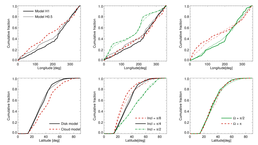
Figure 3.— Variation of final HVS spatial distribution for models H1 (thick lines) and H0.5 (thin lines) with initial binary spatial distribution. We neglect all stars that would be hidden by the Galactic plane, ($\left|b\right|<20^{\circ}$) and reduce statistical weight of stars with $b<0$ by 3 to account for lack of southern hemisphere observations in Brown et al. (2012b) (see their figure 4). Top panels: cumulative fraction of stars vs Galactic longitude. Bottom panels: cumulative fraction vs Galactic latitude. Left: comparison of a thin disc inclined by $45^{\circ}$ with line-of-nodes along $\Omega=120^{\circ}$ with a spherically symmetric initial distribution. Disc geometry causes a clear anisotropy. Middle: dependence on the inclination of the disc plane; modest inclinations do not affect the longitude distribution significantly, while a large inclination results in peaks at $\Omega\pm 90^{\circ}$. Right: dependence on the line-of-nodes position; the position of the longitude peak shifts while the latitude distribution is unaffected.

Figure 4.— Fraction of HVSs as a function of the main sequence lifetime of the primary, binned by $10^{7}$ yr, for models H1 (solid), H0.5 (dashed) and H0.1 (dot-dashed line). The lowest mass supernova progenitors spend $\sim 70$ Myr on main sequence, potentially explaining the HVSs with arrival times close to $10^{8}$ yr.

Although most secondary stars remain bound to the SMBH even after binary disruption, a fraction attains a large enough velocity to escape from the sphere of influence. We give the secondary star ejection probability per SN explosion in the fourth column of Table 1; it ranges from $\sim 4\%$ for unhardened binaries to $\sim 25\%$ for strong hardening. For moderate hardening we find a stellar ejection rate of $\sim 8\times 10^{-6}$ yr^-1.

The production rate of unbound stars is $\sim 3-4$ times higher for binaries with external orbital radii $R\sim 0.1-0.5$ pc, where $v_{\rm ext}\sim v_{\rm int}$, than elsehwere. Closer to the SMBH, $v_{\rm ext}\gg v_{\rm int}$ and the central potential is too deep for stars to easily escape. Further out, external velocities are too low to significantly boost the terminal velocities. Hence, our results are insensitive to the inner and outer disc boundaries.

We present the cumulative distribution of ejected star terminal velocities in Figure 2. In the top panel, we show the distributions as fractions of all ejected stars. This shows that models with stronger hardening not only eject more stars, but also eject them with higher average velocities. In the bottom panel, the distributions are convolved with the supernova rate of $10^{-4}$ yr^-1 and the probabilities of stellar ejection. We also show the HVS production rates predicted by tidal disruption models: Yu & Tremaine (2003), who considered binary injection into low angular momentum orbits due to stellar relaxation only (dashed line labelled ‘YT03’); an equivalent model by Perets et al. (2007), who used a better-constrained binary distribution to find a production rate a factor $10^{3}$ lower (‘P+07, only stars’); and two models from Perets et al. (2007) involving relaxation accelerated by gravitational interactions with massive perturbers such as GMCs (‘P+07, highest rate’ refers to their model GMC1, which gives the highest binary disruption rate and largest number of HVSs, while ‘P+07, S-star match’ refers to model GMC2, which provides the number of S-stars in the central $\sim 0.04$ pc around Sgr A^∗consistent with observations). The two vertical dashed lines represent the velocity cut at $275$ km/s used by Brown et al. (2012b) to identify HVSs and the $400$ km/s Galactic escape velocity used by the same authors. We also give the production probabilities per SN explosion for stars with velocities higher than the two thresholds in Table 1.

In $10^{8}$ years, our models H1, H0.5 and H0.1 predict $37$, $75$ and $512$ stars ejected with terminal velocities $v_{\rm term}>275$ km/s, respectively. These values are somewhat optimistic, because we do not consider deceleration while escaping the Galactic gravitational potential. The latter can be crudely approximated as $\Delta\Phi\sim\sigma^{2}{\rm ln}\left(R/R_{\rm infl}\right)$, with $\sigma=100$ km/s the velocity dispersion in the Galaxy and $R_{\rm infl}\simeq 2$ pc the radius of influence of Sgr A^∗. Taking $R=R_{\rm Solar}=8$ kpc, we find that only stars with $v_{\rm term}\lower 2.15277pt\hbox{$\;\buildrel>\over{\sim}\;$}400$ km/s have radial velocities above the cut at the Solar circle. For these, our models predict $6$, $19$ and $109$ such stars. Therefore, a binary orbit hardening by slightly more than a factor $2$ is enough to produce HVS numbers consistent with observations. In addition, the ratio of unbound to bound HVSs is $\sim 0.3$ in all our models, slightly lower than the observationally derived $\sim 0.5$ (Brown et al., 2012b).

The highest velocities we expect to find in $10^{8}$ yr are $\sim 500$, $\sim 600$ and $\sim 700$ km/s for models H1, H0.5 and H0.1, respectively. Accounting for the deceleration while escaping the galaxy, these velocities are reduced to $\sim 400$, $\sim 530$ and $\sim 640$ km/s, respectively. Such velocities cannot explain the fastest known HVSs, for example US708 with $v_{\rm rf}\simeq 750$ km/s (Hirsch et al., 2005), but the vast majority of currently known ones are moving slower than these maximal radial velocities.

4.3. Spatial distribution of HVSs

Brown et al. (2012b) present observational evidence for anisotropy in the spatial distribution of HVSs (see their Figures 4 and 5). They find a strong excess of HVSs in the Northern galactic hemisphere at longitudes $240^{\circ}<l<300^{\circ}$ and a mild excess at latitudes $45^{\circ}<b<60^{\circ}$. Overall, their result provides a $3\sigma$ confirmation that the HVS distribution is not spherically symmetric.

We produce plots equivalent to Figure 5 from Brown et al. (2012b) in Figure 3 for models H1 and H0.5. We apply a similar a-priori cut as in Brown et al. (2012b): we only consider stars with $\left|b\right|>20^{\circ}$ and reduce the statistical weight of stars with $b<0$ by a factor 3. We consider only stars with terminal velocity $v_{\rm term}>400$ km/s; as we showed above, these stars would have $v_{\rm radial}\sim 275$ km/s at the Solar circle, equivalent to the velocity cut Brown et al. (2012b) used to define HVSs. We compare the HVS distribution obtained from an thin disc with an inclination $i=45^{\circ}$ to the Galactic plane and line-of-nodes direction $\Omega$ pointing toward Galactic longitude $l=120^{\circ}$ with an initially spherically symmetric distribution in the left panels. We find a clear anisotropy caused by the disc. The middle panels show the effects of disc inclination. Angles $i\lesssim 60^{\circ}$ yield a longitude distribution similar to that observed, while $i\simeq 45^{\circ}$ produces a comparable latitude distribution. The effects of the line-of-nodes direction $\Omega$ are shown in the right panels and the longitude distribution can be seen to have a strong peak at $\Omega+\pi/2$ and a weaker one at $\Omega-\pi/2$. The anisotropy is weaker in the H0.5 model than in H1 because hardened binaries have larger internal orbital velocities, weakening the effect of correlated external motions (i.e. the disc). Nevertheless, anisotropy is still present in H0.5. The anisotropy would be amplified if the internal orbits aligned with the disc due to the same torques that cause binary hardening.

4.4. Arrival times

Brown et al. (2012a) recently put constraints on the difference between the stellar age and the travel time from the Galactic centre for five HVSs (the “arrival time”). In our model, arrival time is approximately equal to the main sequence lifetime of the primary star. We plot the fraction of HVSs as a function of the lifetime of the primary star in Figure 4. The main sequence lifetime is given by $t_{\rm MS}\simeq 1.2\times 10^{10}\left(M/{\,{\rm M}_{\odot}}\right)^{-2.5}$ yr and is a very steep function of mass. Stars with $M\simeq 8\;{\,{\rm M}_{\odot}}$ survive for $\sim 70$ Myr and will have been the companions of HVSs with the longest arrival times.

We find $\sim 5-10\%$ of HVSs have companions with main sequence lifetimes $t_{\rm MS}>50$ Myr, within $3\sigma$ of the arrival time results of Brown et al. (2012a). It it also worth noting that massive stars tend to have companions of similar masses (Halbwachs et al., 2003), such that the companions of the most massive stars are more likely to have undergone SNe explosions themselves, reducing the fraction of observable HVSs with short arrival times.

5. Discussion

Our results suggest that supernova-induced disruption of binaries in the Galactic centre can eject stars with rates high enough to explain the majority of the observed HVSs, provided that binaries are hardened compared to their counterparts in the field. We now discuss the processes that potentially lead to binary hardening, the influence of Type Ia supernovae on our results and the fate of undisrupted binaries.

5.1. Binary hardening

Baruteau et al. (2011) present an analysis of binary evolution and migration through gaseous discs. One of the findings is that the disc exerts a torque on the migrating binaries, which hardens them. Typical hardening timescales are a few tens of external orbital times. In our case, the external orbital timescale is $t_{\rm orb}\sim 7500R_{\rm pc}^{3/2}$ yr and binaries are expected to harden on a timescale $t_{\rm harden}\sim 10^{5}$ yr, much shorter than the lifetime of even the most massive stars. This validates our assumption of binary orbits remaining circular after hardening.

Since the hardening torque acts perpendicular to the disc plane, it also works to align the binary internal orbit with its external orbit within the disc. The effect is unlikely to be strong, as the torque direction is essentially random on length scales much smaller than the disc scale height, $H\sim 200R_{\rm pc}$ AU for $H/R=10^{-3}$, but may lead to a weak correlation between internal and external orbital velocity planes. Our calculations show that even a perfect correlation does not increase the stellar ejection rates significantly, however the spatial anisotropy of ejected star directions does become more pronounced.

Another potential binary hardening mechanism is the common envelope phase at the end of the primary’s life. This phase of binary star evolution may occur when the binary separation is of the same order as the primary star’s radius so that the secondary star is engulfed by the envelope of the primary. The binary orbit is then hardened as (internal) orbital energy is used in unbinding the primary’s envelope. The efficiency with which orbital energy is extracted by this process is very uncertain (Ivanova et al., 2013, see e.g. ) and we do not include its effects in our model. However, we note that common envelope evolution would be more frequent in a binary population with orbits hardened via migration through a disc and may play an important role in HVS production.

5.2. Type Ia supernovae

In our calculations, we have considered only core-collapse supernova explosions. White dwarfs in binary systems can explode as Type Ia supernovae; since there is no remnant in that case, the binary disappears and the secondary star can also be ejected from the GC. It is difficult to estimate the rate of these supernovae, because it depends on many parameters of the system, so we cannot constrain the rate of ejection of low-mass stars. Their dynamics, however, are very similar to those presented in this paper. Although the binary components have lower masses, the orbital separations can also be lower due to one binary component being compact, therefore the internal orbital velocities should be comparable. Furthermore, since the secondary star does not need to escape the gravity of the supernova remnant, it loses less orbital energy while leaving the system. Pan et al. (2013) recently interpreted the HVS US708 (Hirsch et al., 2005) as a possible former companion of a Type Ia SN progenitor.

5.3. Pulsars and XRBs in the Galactic Centre

Undisrupted binaries may remain visible as pulsars or X-ray binaries until the secondary star dies. Using an approximate $5\%$ non-disruption probability (see Table 1), we estimate a XRB creation rate $\Gamma_{\rm puls}<10^{-5}$ yr. Typical XRB lifetimes $\lesssim 10^{7}$ yr (King et al., 2001) lead us to predict a population of $<100$ Galactic centre XRBs at any time. This number may be significantly reduced as undisrupted binaries are likely to have eccentric orbits and possibly be prone to tidal disruption. The fate of XRBs and the remnants in general is complicated by stellar dynamics within the GC, binary evolution and accretion physics and we intend to examine these issues in future work.

6. Conclusions

We have used a Monte Carlo model to examine the effects of core-collapse SN explosions in binary stars in orbit around Sgr A^∗. We calculate the post-SN orbits of the binary members and find that most binaries get disrupted, with some secondary stars escaping the gravity of Sgr A^∗. The binary disruption rate is $\sim 10^{-4}$ yr^-1, comparable to tidal disruption models. Stellar ejection rates depend on the degree of binary hardening, which may occur during migration in the gaseous disc from which the binary stars formed. Three cases - no hardening, moderate hardening (binary separation reduced by a factor 2) and strong hardening (reduction by 10) give ejection rates of $4$, $7$ and $22\times 10^{-6}$ yr, respectively. Of these stars, a fraction would have terminal velocities large enough to be classed as HVSs observationally. For the three models, we estimate HVS populations of $37$, $75$ and $512$ stars respectively, although these numbers are certainly optimistic.

Our models also preserve the spatial anisotropy of the original stellar population. However, stronger binary hardening increases the HVS production rate at the expense of dampening the spatial anisotropy. Taking these factors together requires massive binaries formed in the few central parsecs of the Galactic centre to have had typical separations a factor 2 less than those in the field at the point just prior to the supernova explosion. This constraint would be significantly weakened if the hardening process also caused the binary orbital planes to become somewhat correlated with the plane of the stellar disc, thus helping to preserve the spatial anisotropy of the ejected HVSs. We note that the similar HVS production rates predicted by the SN-induced and tidal disruption models mean that both mechanisms likely contribute to the observed HVS population.

We thank Sergei Nayakshin and Richard Alexander for helpful discussions. Astrophysics research at the University of Leicester is supported by the STFC.

References

- Abadi et al. (2009) Abadi, M. G., Navarro, J. F., & Steinmetz, M. 2009, ApJ, 691, L63
- Arzoumanian et al. (2002) Arzoumanian, Z., Chernoff, D. F., & Cordes, J. M. 2002, ApJ, 568, 289
- Baruteau et al. (2011) Baruteau, C., Cuadra, J., & Lin, D. N. C. 2011, ApJ, 726, 28
- Blaauw (1961) Blaauw, A. 1961, Bull. Astr. Inst. Netherlands, 15, 265
- Blum et al. (2003) Blum, R. D., Ramírez, S. V., Sellgren, K., & Olsen, K. 2003, ApJ, 597, 323
- Bromley et al. (2009) Bromley, B. C., Kenyon, S. J., Brown, W. R., & Geller, M. J. 2009, ApJ, 706, 925
- Brown et al. (2010) Brown, W. R., Anderson, J., Gnedin, O. Y., et al. 2010, ApJ, 719, L23
- Brown et al. (2012a) Brown, W. R., Cohen, J. G., Geller, M. J., & Kenyon, S. J. 2012a, ApJ, 754, L2
- Brown et al. (2012b) Brown, W. R., Geller, M. J., & Kenyon, S. J. 2012b, ApJ, 751, 55
- Brown et al. (2009) Brown, W. R., Geller, M. J., Kenyon, S. J., & Bromley, B. C. 2009, ApJ, 690, L69
- Brown et al. (2005) Brown, W. R., Geller, M. J., Kenyon, S. J., & Kurtz, M. J. 2005, ApJ, 622, L33
- Brown et al. (2007) Brown, W. R., Geller, M. J., Kenyon, S. J., Kurtz, M. J., & Bromley, B. C. 2007, ApJ, 671, 1708
- Dray et al. (2005) Dray, L. M., Dale, J. E., Beer, M. E., Napiwotzki, R., & King, A. R. 2005, MNRAS, 364, 59
- Gillessen et al. (2009) Gillessen, S., Eisenhauer, F., Trippe, S., et al. 2009, ApJ, 692, 1075
- Gualandris et al. (2005) Gualandris, A., Portegies Zwart, S., & Sipior, M. S. 2005, MNRAS, 363, 223
- Gvaramadze & Gualandris (2011) Gvaramadze, V. V., & Gualandris, A. 2011, MNRAS, 410, 304
- Gvaramadze et al. (2009) Gvaramadze, V. V., Gualandris, A., & Portegies Zwart, S. 2009, MNRAS, 396, 570
- Halbwachs et al. (2003) Halbwachs, J. L., Mayor, M., Udry, S., & Arenou, F. 2003, A&A, 397, 159
- Heber et al. (2008) Heber, U., Edelmann, H., Napiwotzki, R., Altmann, M., & Scholz, R.-D. 2008, A&A, 483, L21
- Hills (1983) Hills, J. G. 1983, ApJ, 267, 322
- Hills (1988) —. 1988, Nature, 331, 687
- Hirsch et al. (2005) Hirsch, H. A., Heber, U., O’Toole, S. J., & Bresolin, F. 2005, A&A, 444, L61
- Hobbs et al. (2005) Hobbs, G., Lorimer, D. R., Lyne, A. G., & Kramer, M. 2005, MNRAS, 360, 974
- Irrgang et al. (2010) Irrgang, A., Przybilla, N., Heber, U., Nieva, M. F., & Schuh, S. 2010, ApJ, 711, 138
- Irrgang et al. (2013) Irrgang, A., Wilcox, B., Tucker, E., & Schiefelbein, L. 2013, A&A, 549, A137
- Ivanova et al. (2013) Ivanova, N., Justham, S., Chen, X., et al. 2013, A&A Rev., 21, 59
- King et al. (2001) King, A. R., Davies, M. B., Ward, M. J., Fabbiano, G., & Elvis, M. 2001, ApJ, 552, L109
- Kobulnicky & Fryer (2007) Kobulnicky, H. A., & Fryer, C. L. 2007, ApJ, 670, 747
- Kollmeier et al. (2009) Kollmeier, J. A., Gould, A., Knapp, G., & Beers, T. C. 2009, ApJ, 697, 1543
- Leonard (1991) Leonard, P. J. T. 1991, AJ, 101, 562
- Limongi & Chieffi (2009) Limongi, M., & Chieffi, A. 2009, Memm. della SAI, 80, 151
- Lu et al. (2010) Lu, Y., Zhang, F., & Yu, Q. 2010, ApJ, 709, 1356
- Nayakshin (2006) Nayakshin, S. 2006, MNRAS, 372, 143
- Pan et al. (2013) Pan, K.-C., Ricker, P., & Taam, R. 2013, ArXiv e-prints, arXiv:1303.1228
- Paumard et al. (2006) Paumard, T., Genzel, R., Martins, F., et al. 2006, ApJ, 643, 1011
- Perets et al. (2009) Perets, H. B., Gualandris, A., Kupi, G., Merritt, D., & Alexander, T. 2009, ApJ, 702, 884
- Perets et al. (2007) Perets, H. B., Hopman, C., & Alexander, T. 2007, ApJ, 656, 709
- Piffl et al. (2011) Piffl, T., Williams, M., & Steinmetz, M. 2011, A&A, 535, A70
- Portegies Zwart (2000) Portegies Zwart, S. F. 2000, ApJ, 544, 437
- Przybilla et al. (2008) Przybilla, N., Nieva, M. F., Heber, U., & Butler, K. 2008, ApJ, 684, L103
- Raguzova & Popov (2005) Raguzova, N. V., & Popov, S. B. 2005, Astronomical and Astrophysical Transactions, 24, 151
- Sana et al. (2012) Sana, H., de Mink, S. E., de Koter, A., et al. 2012, Science, 337, 444
- Tillich et al. (2009) Tillich, A., Przybilla, N., Scholz, R.-D., & Heber, U. 2009, A&A, 507, L37
- Woosley et al. (2002) Woosley, S. E., Heger, A., & Weaver, T. A. 2002, Reviews of Modern Physics, 74, 1015
- Yu & Tremaine (2003) Yu, Q., & Tremaine, S. 2003, ApJ, 599, 1129
- Zhang et al. (2013) Zhang, F., Lu, Y., & Yu, Q. 2013, ApJ, 768, 153