Critical behavior of the fidelity susceptibility for the $d=2$ transverse-field Ising model

Abstract

The overlap (inner product) between the ground-state eigenvectors with proximate interaction parameters, the so-called fidelity, plays a significant role in the quantum-information theory. In this paper, the critical behavior of the fidelity susceptibility is investigated for the two-dimensional tranverse-field (quantum) Ising model by means of the numerical diagonalization method. In order to treat a variety of system sizes $N=12,14,\dots,32$, we adopt the screw-boundary condition. Finite-size artifacts (scaling corrections) of the fidelity susceptibility appear to be suppressed, as compared to those of the Binder parameter. As a result, we estimate the fidelity-susceptibility critical exponent as $\alpha_{F}=0.715(20)$.

1 Introduction

In the quantum-information theory, the inner product (overlap) between the ground-state eigenvectors

$$F(\Gamma,\Gamma+\Delta\Gamma)=|\langle\Gamma|\Gamma+\Delta\Gamma\rangle|,$$ (1)

for proximate interaction parameters, $\Gamma$ and $\Gamma+\Delta\Gamma$, the so-called fidelity [1, 2], provides valuable information as to a distinguishability of quantum states. The idea of fidelity also plays a significant role in the quantum dynamics [3] as a measure of tolerance for external disturbances; see Ref. [4] for a review.

As would be apparent from the definition (1), the fidelity suits the numerical-exact-diagonalization calculation, for which an explicit expression for $|\Gamma\rangle$ is available. At finite temperatures, the above definition, Eq. (1), has to be modified accordingly, and the modified version of $F$ is readily calculated with the quantum Monte Carlo method [5, 6, 7].

Meanwhile, the fidelity (1) tuned out to be sensitive to an onset of criticality [8, 9, 10]; see Ref. [11] for a review. To be specific, for a finite-size cluster with $N$ spins, the fidelity susceptibility

$$\chi_{F}=\frac{1}{N}\partial^{2}_{\Delta\Gamma}F|_{\Delta\Gamma=0},$$ (2)

exhibits a notable singularity at a critical point. Because the tractable system size with the numerical-exact-diagonalization method is restricted severely, an alternative scheme for criticality might be desirable to complement traditional ones. In fact, the quantum-Monte-Carlo algorithm applies successfully [6] to the analysis of $\chi_{F}$ for the $d=2$ transverse-field Ising model with $N\leq 48\times 48$ spins. However, for the frustrated magnetism, the quantum-Monte-Carlo method suffers from the negative-sign problem. On the contrary, the numerical diagonalization method is free from such difficulty, permitting us to consider a wide range of intriguing topics.

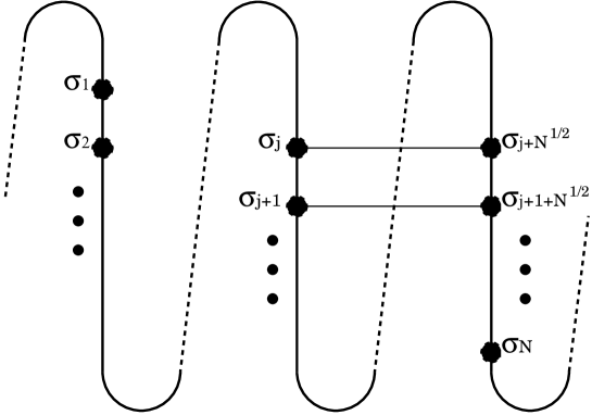
Figure 1: Imposing the screw-boundary condition [12, 13], we construct the finite-size cluster for the two-dimensional transverse-field Ising model (3) with $N$ spins. As indicated above, the spins constitute a $d=1$-dimensional alignment $\{\sigma_{i}\}$ ($i=1,2,\dots,N$), and the dimensionality is lifted to $d=2$ by the bridges (long-range interactions) over the ($N^{1/2}$)th-neighbor pairs. The simulation algorithm is explained in Sec. 2.1.

In this paper, we calculated the fidelity susceptibility (2) for the two-dimensional transverse-field (quantum) Ising model (3) by means of the numerical diagonalization method. In order to treat a variety of system sizes, $N=12,14,\dots,32$, systematically, we implemented the screw-boundary condition with the aid of Novotny’s method [12, 13]; see Fig. 1. So far, the fidelity susceptibility has been calculated [14] for $N=10,16,18$, and $20$. As a comparison, we calculated the Binder parameter [15] to determine the location of the critical point. As a matter of fact, it has been known that owing to the screw-boundary condition, the simulation result suffers from a slowly undulating deviation with respect to $N$ [12]; namely, for a quadratic value of $N=16,25$, the amplitude of deviation gets enhanced. Such a notorious wavy deviation seems to be suppressed for $\chi_{F}$; the fidelity susceptibility may serve a promising candidate for the numerical analysis of critical phenomena.

To be specific, the Hamiltonian for the two-dimensional transverse-field Ising model is given by

$${\cal H}=-\sum_{\langle ij\rangle}\sigma^{z}_{i}\sigma^{z}_{j}-\Gamma\sum_{i}^{N}\sigma^{x}_{i}.$$ (3)

Here, the Pauli operator $\{\vec{\sigma}_{i}\}$ is placed at each two-dimensional- (square-) lattice point $i$. The summation $\sum_{\langle ij\rangle}$ runs over all possible nearest-neighbor pairs $\langle ij\rangle$. The parameter $\Gamma$ denotes the transverse magnetic field. Upon increasing $\Gamma$, a phase transition between the ferro- and para-magnetic phases takes place at $\Gamma_{c}=3.04497(19)$ [16]; see Ref. [17] as well. Our aim is to investigate the critical behavior of the fidelity susceptibility [14]

$$\chi_{F}\sim|\Gamma-\Gamma_{c}|^{-\alpha_{F}},$$ (4)

with the critical exponent $\alpha_{F}$. As a byproduct, we calculated the correlation-length critical exponent $\nu$ through resorting to the scaling relation advocated in Ref. [6]; to avoid a confusion as to the definition of $\nu$, we refer readers to a brief remark [18].

The rest of this paper is organized as follows. In Sec. 2, we investigate the critical behavior of the fidelity susceptibility (2) with the numerical diagonalization method; a brief account for the simulation scheme is given as well. In Sec. 3, we show the summary and discussions.

2 Numerical results

In this section, we present the numerical result for the transverse-field Ising model (3). For the sake of self-consistency, we give a brief account for the simulation scheme, namely, Novotny’s method [12, 13], to implement the screw-boundary condition (Fig. 1). This simulation method allows us to treat a variety of system sizes $N=12,14,\dots,32$ in a systematic manner. The linear dimension $L$ of the cluster is given by

$$L=\sqrt{N},$$ (5)

because $N$ spins constitute a rectangular cluster.

2.1 Simulation method: Screw-boundary condition

In this section, we explain the simulation scheme to implement the screw-boundary condition. Our scheme is based on Novotny’s method [12, 13], which was developed for the transfer-matrix simulation of the classical Ising model. In order to adapt this method for the quantum-mechanical counterpart, a slight modification has to be made. Here, we present a brief, albeit, mathematically closed, account for the simulation algorithm.

Before commencing an explanation of the technical details, we sketch a basic idea of Novotny’s method. We consider a finite-size cluster as shown in Fig. 1. We place an $S=1/2$ spin (Pauli operator $\vec{\sigma}_{i}$) at each lattice point $i(\leq N)$. Basically, the spins constitute a one-dimensional ($d=1$) structure. The dimensionality is lifted to $d=2$ by the long-range interactions over the $\sqrt{N}$-th-neighbor distances; owing to the long-range interaction, the $N$ spins form a $\sqrt{N}\times\sqrt{N}$ rectangular network effectively.

According to Novotny [12, 13], the long-range interactions are introduced systematically by the use of the translation operator $P$; see Eq. (9). The operator $P$ satisfies the formula

$$P|\sigma_{1},\sigma_{2},\dots,\sigma_{N}\rangle=|\sigma_{N},\sigma_{1},\dots,\sigma_{N-1}\rangle.$$ (6)

Here, the Hilbert-space bases $\{|\sigma_{1},\sigma_{2},\dots,\sigma_{N}\rangle\}$ ($\sigma_{i}=\pm 1$) diagonalize the longitudinal component $\sigma^{z}_{i}$ of the Pauli operator;

$$\sigma_{j}^{z}|\{\sigma_{i}\}\rangle=\sigma_{j}|\{\sigma_{i}\}\rangle.$$ (7)

The Hamiltonian is given by

$${\cal H}=-\left[H\left(1\right)+H\left(\sqrt{N}\right)\right]-\Gamma\sum_{i=1}^{N}\sigma^{x}_{i},$$ (8)

Here, the matrix $H(v)$ denotes the $v$-th neighbor interaction. The matrix $H(v)$ is diagonal, and the diagonal element is given by

$$H_{\{\sigma_{i}\},\{\sigma_{i}\}}(v)=\langle\{\sigma_{i}\}|H(v)|\{\sigma_{i}\}\rangle=\langle\{\sigma_{i}\}|TP^{v}|\{\sigma_{i}\}\rangle.$$ (9)

The insertion of $P^{v}$ is a key ingredient to introduce the $v$-th neighbor interaction. Here, the matrix $T$ denotes the exchange interaction between $\{\sigma_{i}\}$ and $\{\tau_{i}\}$; namely, the matrix element of $T$ is given by

$$\langle\{\sigma_{i}\}|T|\{\tau_{i}\}\rangle=\sum_{k=1}^{N}\sigma_{k}\tau_{k}.$$ (10)

The above formulae complete the formal basis of our simulation scheme. We diagonalize the Hamiltonian matrix (8) for $N\leq 32$ spins numerically. In the practical numerical calculation, however, a number of formulas may be of use; see the Appendices of Refs. [19, 20].

2.2 Analysis of the critical point with the fidelity susceptibility $\chi_{F}$ and Binder’s parameter $U$

In Fig. 2, we present the fidelity susceptivity $\chi_{F}$ (2) for various $\Gamma$ and $N=12,14,\dots,32$. Around $\Gamma\approx 3$, there appears a clear signature of criticality; in Ref. [14], the criticality was analyzed for $N=10,16,18$ and $20$. Our aim is to survey the critical behavior of $\chi_{F}$ for extended system sizes $N\leq 32$.

In Fig. 3, we plot the approximate critical point $\Gamma_{c}(L)$ (plusses) for $1/L^{2}(=1/N)$; the range of $N$ is the same as that of Fig. 2. Here, the approximate critical point denotes the location of maximal $\chi_{F}$; namely, the relation

$$\partial_{\Gamma}\chi|_{\Gamma=\Gamma_{c}(L)}=0,$$ (11)

holds. The series of $\Gamma_{c}(L)$ appears to exhibits a wavy (slowly undulating) deviation with respect to $L(=\sqrt{N})$. Such a wavy character is attributed to an artifact of the screw-boundary condition [12]; namely, the deviation amplitude is suppressed for quadratic values of $N=16,25$ (commensurate condition). The least-squares fit to the data in Fig. 3 yields an estimate $\Gamma_{c}=2.965(46)$ in the thermodynamic limit. The result is consistent with a preceding estimate $\Gamma_{c}=2.95(1)$ [14]. A large-scale numerical-exact-diagonalization result $\Gamma_{c}=3.04497(19)$ for $N\leq 6\times 6$ [16] lies out of the error margin. Possibly, the abscissa scale $1/L^{2}$ in Fig. 3, namely, the power-law singularity of corrections to scaling, has to be finely-tuned in order to better attain precise extrapolation to the thermodynamic limit. Nevertheless, the extrapolated critical point $\Gamma_{c}$ is no longer used in the subsequent analyses, and we do not go into further details; rather, the approximate critical point $\Gamma_{c}(L)$ is fed into the formula, Eq. (15).

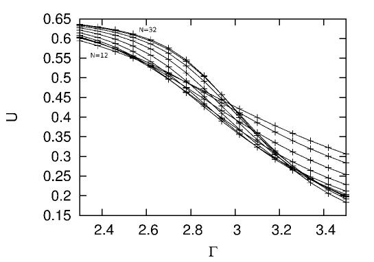
Figure 4: The Binder parameter $U$ (12) is plotted for various $\Gamma$ and $N=12,14,\dots,32$. The intersection point of the curves indicates a location of the critical point $\Gamma_{c}(L)$ (14), which is shown in Fig. 3.

As a comparison, we provide an alternative analysis of $\Gamma_{c}$ via the Binder parameter [15]. In Fig. 4, we present the Binder parameter

$$U=1-\frac{\langle\Gamma|M^{4}|\Gamma\rangle}{3\langle\Gamma|M^{2}|\Gamma\rangle^{2}},$$ (12)

with the magnetic moment

$$M=\sum_{i=1}^{N}\sigma^{z}_{i},$$ (13)

for various $\Gamma$ and $N=12,14,\dots,32$. The intersection point of the curves indicates a location of criticality. Because of the above-mentioned wavy deviation, the location of the intersection point becomes unclear.

In Fig. 3, we plot the approximate critical point $\Gamma_{c}(L)$ (crosses) for $1/L^{2}$. Here, the approximate critical point denotes an intersection point of the Binder-parameter curves with respect to a pair of system sizes $N=L^{2}-1$ and $L^{2}+1$. Namely, the following relation holds:

$$U(L^{2}-1)|_{\Gamma=\Gamma_{c}(L)}=U(L^{2}+1)_{\Gamma=\Gamma_{c}(L)}.$$ (14)

The finite-size deviation of $U$ appears to be much larger than that of $\chi_{F}$. As mentioned above, such a wavy character is attributed to an artifact of the screw-boundary condition [12]. Namely, the deviation amplitude gets enhanced for quadratic values of $N=16,25$. The least-squares fit to these data yields an estimate $\Gamma_{c}=3.89(31)$ in the thermodynamic limit $L\to\infty$. The pronounced finite-size deviation prohibits us from analyzing the criticality reliably.

We address a remark. As mentioned above, the oscillatory-deviation amplitude depends on the condition whether the system size $L(=\sqrt{N})$ is close to an integral number (commensurate) or not (incommensurate). One is able to reduce the oscillatory deviation by tuning the screw pitch for each $N$ [21]. Such an elaborate treatment might be worth pursuing to better attain precise estimation of critical indices.

2.3 Fidelity-susceptibility critical exponent $\alpha_{F}$

In this section, we analyze the fidelity-susceptibility critical exponent $\alpha_{F}$ with the finite-size-scaling method. As a byproduct, we estimate the correlation-length critical exponent $\nu$.

In Fig. 5, we plot the logarithm of $\chi_{F}$ at the approximate critical point, namely,

$$\ln\chi_{F}|_{\Gamma=\Gamma_{c}(L)},$$ (15)

against $\ln L$ for $N=12,14,\dots,32$ ($L=\sqrt{N}$). According to the finite-size scaling, at the critical point, (the singular part of) the susceptibility obeys the power law $\chi_{F}\sim L^{\alpha_{F}/\nu}$ with the correlation-length critical exponent $\nu$; see Ref. [18] as well. Therefore, the slope of $\ln L$-$\ln\chi_{F}|_{\Gamma=\Gamma_{c}(L)}$ data indicates the critical exponent $\alpha_{F}/\nu$. The least-squares fit to the data in Fig. 5 yields $\alpha_{F}/\nu=1.113(49)$. This result is to be compared with the preceding one $\alpha_{F}/\nu=1.02$ [14] for $N=10,16,18$ and $20$. The series of data in Fig. 5 exhibit a slowly undulating deviation inherent in the screw-boundary condition. As mentioned above, the deviation amplitude depends on the condition whether the system size $L(=\sqrt{N})$ is close to an integral number (commensurate) or not (incommensurate). The system size $12\leq N\leq 32$ in Fig. 5 covers one period in the sense that the difference of the system size $\sqrt{32}-\sqrt{12}\approx 2.2$ is close to two (an even number); owing to the cancellation over one period, the result $\alpha_{F}/\nu=1.113(49)$ might not be affected by the oscillatory deviation very much. As a reference, we provide an alternative analysis of $\alpha_{F}/\nu$. As mentioned above, the commensurate series $N=16,24,26$ and the incommensurate one $N=12,14,30,32$ behave differently. Among the pairs $(N_{1},N_{2})$ ($L_{1,2}=\sqrt{N_{1,2}}$) within each series, we calculate the exponent

$$\alpha_{F}/\nu=\frac{\ln\chi_{F}(L_{1})|_{\Gamma=\Gamma_{c}(L_{1})}-\ln\chi_{F}(L_{2})|_{\Gamma=\Gamma_{c}(L_{2})}}{\ln L_{1}-\ln L_{2}}.$$ (16)

For the commensurate-series pairs, $(N_{1},N_{2})=(16,24)$ and $(16,26)$, we arrive at $\alpha_{F}/\nu=1.126$ and $1.068$, respectively. Similarly, for the incommensurate-series pairs, $(12,14)$, $(30,32)$, $(12,30)$, $(14,32)$, and $(12,32)$, we obtain $\alpha_{F}/\nu=1.191$, $1.157$, $1.133$, $1.124$, and $1.135$, respectively. The least-squares fit to these data with the abscissa scale $1/(N_{1}+N_{2})^{2}$ yields $\alpha_{F}/\nu=1.10(3)$ in the thermodynamic limit $N\to\infty$. This result confirms the above preliminary result $\alpha_{F}/\nu=1.113(49)$; hereafter, we accept $\alpha_{F}/\nu=1.113(49)$, aiming to estimate related scaling indices. Nevertheless, we stress that a rather moderate cluster size already reaches the scaling regime, as noted in Ref. [14].

We are able to estimate the respective indices, $\alpha_{F}$ and $\nu$, through resorting to a number of scaling relations. According to the scaling argument [6], the index $\alpha_{F}$ satisfies the relation

$$\alpha_{F}=\alpha+\nu,$$ (17)

with the specific-heat critical exponent $\alpha$. On the one hand, the hyper-scaling theory insists that the specific-heat critical exponent satisfies the relation $\alpha=2-D\nu$ with the spatial and temporal dimensionality $D=2+1$. Putting the present estimate $\alpha_{F}/\nu=1.113(49)$ into the above scaling relations, we arrive at $\alpha_{F}=0.715(20)$ and $\nu=0.642(10)$. The former is in good agreement with the preceding estimate $\alpha_{F}=0.73$ [14] for $N=10,16,18$ and $20$. The latter lies slightly out of a recent Monte Carlo result $\nu=0.63020(12)$ [22] for the three-dimensional classical Ising model; the universality class of the ground-state phase transition for the two-dimensional transverse-field Ising model belongs to the three-dimensional classical counterpart. Again, it is suggested that the $\chi_{F}$-based finite-size scaling analysis is less influenced by corrections to scaling. In particular, an agreement with $\alpha_{F}=0.73$ [14] confirms that a rather moderate system size $N\approx 4\times 4$ already reaches the scaling regime.

3 Summary and discussions

The critical behavior of the fidelity susceptibility (2) was investigated for the two-dimensional transverse-field Ising model (3) by means of the numerical diagonalization method. In order to treat a variety of system sizes $N=12,14,\dots,32$, we implemented the screw-boundary condition (Sec. 2.1) with the aid of Novotny’s method [12, 13].

The fidelity susceptibility exhibits a notable singularity (Fig. 2), with which we estimated the critical point as $\Gamma_{c}=2.965(46)$ (Fig. 3). Moreover, scrutinizing its power-law singularity at the critical point (Fig. 5), we obtained the critical exponent $\alpha_{F}=0.715(20)$. These results are to be compared with the preceding estimates [14], $\Gamma_{c}=2.95(1)$ and $\alpha_{F}=0.73$, obtained for $N=10,16,18$ and $20$. Hence, it is suggested that the simulation results for rather small clusters already reach the scaling regime. As a byproduct, through the scaling relation (17) [6], we arrive at $\nu=0.642(10)$. According to an extensive Monte Carlo simulation for the three-dimensional classical Ising model [22], the correlation-length critical exponent was estimated as $\nu=0.63020(12)$; this value lies slightly out of the error margin. Again, it is suggested that the analysis via $\chi_{F}$ might be less influenced by corrections to scaling (systematic errors). As mentioned in Introduction, the quantum-Monte-Carlo method is also a clue to the analysis of the fidelity susceptibility. Actually, a considerably precise result $\nu=0.625(3)$ was reported in Ref. [6].

By definition (1), the fidelity susceptivity suits the numerical diagonalization calculation. Because the tractable system size with the numerical diagonalization method is severely restricted, such an alternative scheme might be desirable to complement the existing ones. It would be tempting to apply the fidelity susceptibility to a wide class of systems of current interest such as the frustrated quantum magnetism, for which the Monte Carlo method suffers from the negative-sign problem. This problem would be addressed in the future presentation.

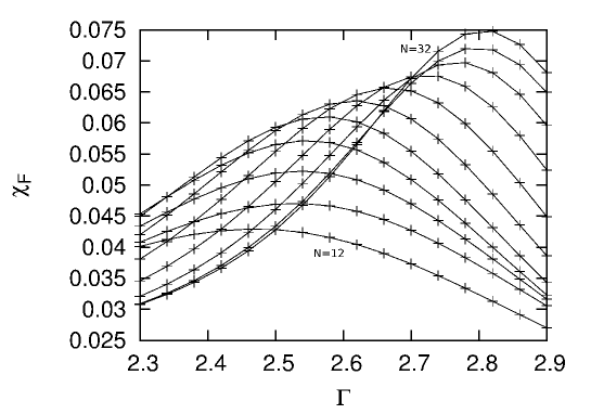
Figure 2: The fidelity susceptibility $\chi_{F}$ (2) is plotted for various $\Gamma$ and $N=12,14,\dots,32$. A notable singularity emerges at $\Gamma\approx 3$. The drift of $\Gamma_{c}$ is analyzed in Fig. 3.

Figure 3: The approximate critical point $\Gamma_{c}(L)$ determined via $\chi_{F}$ (plusses) [Eq. (11)] and $U$ (crosses) [Eq. (14)] is plotted for $1/L^{2}$. The least-squares fit to these data yields $\Gamma_{c}=2.965(46)$ and $3.89(31)$, respectively, in the thermodynamic limit $L\to\infty$. The series of data exhibit a slowly undulating deviation intrinsic to the screw-boundary condition [12]; that is, for quadratic values of $N=16$ and $25$, the deviation amplitude gets enhanced.

Figure 5: The logarithm of the fidelity susceptibility at the approximate critical point, namely, $\ln\chi_{F}|_{\Gamma=\Gamma_{c}(L)}$, is plotted against $\ln L$ for $N=12,14,\dots,32$ ($L=\sqrt{N}$). The slope of the series of data indicates the critical exponent $\alpha_{F}/\nu$. The least-squares fit to these data yields an estimate $\alpha_{F}/\nu=1.113(49)$. A further consideration of the respective indices, $\alpha_{F}$ and $\nu$, is made in the text.

References

- [1] A. Uhlmann, Rep. Math. Phys. 9 (1976) 273.
- [2] R. Jozsa, J. Mod. Opt. 41 (1994) 2315.
- [3] A. Peres, Phys. Rev. A 30 (1984) 1610.
- [4] T. Gorin, T. Prosen, T. H. Seligman, and M. Žnidarič, Phys. Rep. 435 (2006) 33.
- [5] D. Schwandt, F. Alet, and S. Capponi, Phys. Rev. Lett. 103 (2009) 170501.
- [6] A. F. Albuquerque, F. Alet, C. Sire, and S. Capponi, Phys. Rev. B 81 (2010) 064418.
- [7] C. De Grandi, A. Polkovnikov, and A. W. Sandvik, Phys. Rev. B 84 (2011) 224303.
- [8] H. T. Quan, Z. Song, X. F. Liu, P. Zanardi, and C. P. Sun, Phys. Rev. Lett. 96 (2006) 140604.
- [9] P. Zanardi and N. Paunković, Phys. Rev. E 74 (2006) 031123.
- [10] H.-Q. Zhou, and J. P. Barjaktarevic̃, J. Phys. A: Math. Theor. 41 (2008) 412001.
- [11] V. R. Vieira, J. Phys: Conference Series 213 (2010) 012005.
- [12] M.A. Novotny, J. Appl. Phys. 67 (1990) 5448.
- [13] M.A. Novotny, Phys. Rev. B 46 (1992) 2939.
- [14] W.-C. Yu, H.-M. Kwok, J. Cao, and S.-J. Gu, Phys. Rev. E 80 (2009) 021108.
- [15] K. Binder, Phys. Rev. Lett. 47 (1981) 693.
- [16] C. J. Hamer, J. Phys. A 33 (2000) 6683.
- [17] M. Henkel, J. Phys. A 20 (1987) 3969.
- [18] S.-J. Gu, H.-M. Kwok, W.-Q. Ning, and H.-Q. Lin, Phys. Rev. B 77 (2008) 245109; ibid. 83 (2011) 159905(E).
- [19] Y. Nishiyama, Phys. Rev. E 75 (2007) 051116.
- [20] Y. Nishiyama, Nucl. Phys. B 832 (2010) 605.
- [21] Y. Nishiyama, J. Stat. Mech. (2011) P08020.
- [22] Y. Deng and H. W. J. Blöte, Phys. Rev. E 68 (2003) 036125.