Quantum Energy Teleportation without Limit of Distance

Abstract

Quantum energy teleportation (QET) is, from the operational viewpoint of distant protocol users, energy transportation via local operations and classical communication. QET has various links to fundamental research fields including black hole physics, the quantum theory of Maxwell’s demon, and quantum entanglement in condensed matter physics. However, the energy that has been extracted using a previous QET protocol is limited by the distance between two protocol users; the upper bound of the energy being inversely proportional to the distance. In this letter, we prove that introducing squeezed vacuum states with local vacuum regions between the two protocol users overcomes this limitation, allowing energy teleportation over practical distances.

I Introduction

Quantum fields in the vacuum state accompany spatially entangled energy density fluctuations via the noncommutativity of energy density operators. However, the eigenvalue of the total Hamiltonian can be set to zero by discarding the zero-point energy, primarily because this energy exhibits the fundamental property known as passivity passivity and is of little use; any intended local operation for extracting the zero-point energy out of a field actually injects energy and excites the vacuum. The zero-point energy, however, can be glimpsed through a spatial region with negative energy density BD , along with the Casimir effect C and the Unruh effect UW . In such a spatial region, the quantum field can afford to attain a lower energy density than the zero value of the vacuum state because it saves the zero-point energy in the vacuum state. Of course, we have another region with sufficient positive energy to ensure that the total energy is greater than zero.

Recently, quantum information theory has revealed some exotic aspects of the entangled energy density fluctuation of many-body systems in the ground state, and it has been proven that quantum energy teleportation (QET) is possible QET ; bh . QET is, from the operational viewpoint of distant protocol users, energy transportation via local operations and classical communication (LOCC). In contrast to the standard protocols of quantum teleportation qt , QET protocols involve energy transportation. QET is related to the quantum theory of Maxwell’s demon at low temperatures fgh and the local cooling problem of many-body quantum systems sc . Furthermore, QET provides insight into the black hole entropy problem bh . QET can be implemented in various research fields including spin chains sc , harmonic chains hc , and cold trapped ions coti . Although QET has not yet been experimentally verified, a realistic experiment was recently proposed yih ; the experiment uses 1+1-dimensional chiral massless boson fields of quantum Hall edge currents yoshioka , and the teleported energy may be expected to take values near $O(100)~{}\mu$eV with present technology.

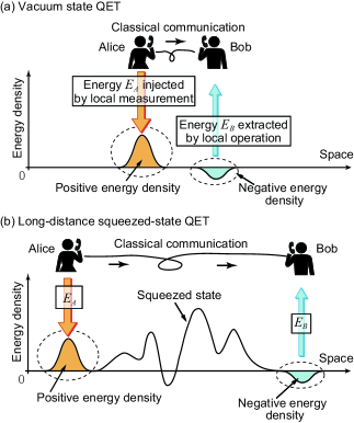
Figure 1: (Color online) Schematic diagram of (a) vacuum state quantum energy teleportation (QET) protocol and (b) long-distance squeezed-state QET.

Despite such experimental proposals for various physical systems sc ; hc ; coti ; yih , a strong distance limitation has hampered experimental verification; in QET over a distance $L$, the transferred energy $E_{B}$ of 1+1 dimensional massless scalar fields is bounded by

$$E_{B}\leq\frac{1}{12\pi L},$$ (1)

as long as vacuum-state QET protocols are adopted. Here, the natural unit $c=\hbar=1$ is adopted. QET thus sends only a small amount of energy over a long distance $L$. This vacuum-state QET distance bound appears for two reasons: From an informational viewpoint, the spatial correlations of the zero-point fluctuation, including quantum entanglement, decay as the distance becomes large, and hence the amount of information for distant control of a quantum fluctuation becomes small and only weak strategies for extracting energy out of the distant zero-point fluctuation are available. From a physical viewpoint, the localized negative energy induced by a QET protocol cannot be separated from the positive energy injected by the measurement device; otherwise, the negative energy excitation would exist without any positive energy excitations. To make the total energy of the field nonnegative, the negative energy excitation requires a sufficient amount of positive energy at a close distance. However, there is an interesting possibility that avoids this bound by using an exotic quantum state for QET, as we argue in this paper.

We propose here a new version of the QET protocols that use a squeezed vacuum state in place of the vacuum state between two protocol users (Fig. 1). In our proposal, the spatial correlation of the quantum fluctuations with zero energy is maintained even if the distance between the sender and receiver of QET is very large. The negative energy induced by the extraction of positive energy via QET is sustained not by the positive energy injected by the measurement but instead by the excitation energy in the squeezed region of the state. Thus, the bound in Eq. (1) is overcome and long-distance energy teleportation can be achieved. The protocol may be implemented by adopting a spatial expansion method, which is one strategy for realizing a long-distance correlation, thus facilitating experimental verification of QET and potentially contributing to quantum device applications.

The paper is organized as follows. In Section 2, a brief review of vacuum-state QET is provided, and in Section 3, the distance bound in Eq. (1) is derived. In Section 4, using a squeezed state, we outline the new protocol that realizes QET without the limit of distance. The results are summarized in Section 5.

II
Brief Review of Vacuum-State QET

Recalling the experimental proposal using quantum Hall edge currents yih , let us consider a free massless scalar quantum field $\hat{\varphi}$ in 1+1 dimensions that obeys the equation of motion

$$\left(\partial_{t}^{2}-\partial_{x}^{2}\right)\hat{\varphi}=0.$$

The general solution is obtained as the sum of a left-moving component $\hat{\varphi}_{+}(x^{+})~{}$and a right-moving component $\hat{\varphi}_{-}(x^{-})~{}$using the light-cone coordinates $x^{\pm}=t\pm x$. For the purposes of our discussion, we can focus solely on the left mover $\hat{\varphi}_{+}(x^{+})$. In quantum Hall systems, $\hat{\varphi}_{+}(x^{+})$ describes the charge density fluctuation of the edge yoshioka . The energy flux operator is given by

$$\hat{T}_{++}(x^{+})=:\hat{\Pi}_{+}(x^{+})^{2},$$

where $\hat{\Pi}_{+}(x^{+})=\partial_{x^{+}}\hat{\varphi}_{+}(x^{+})$, and the total energy operator is calculated as

$$\hat{H}_{+}=\int_{-\infty}^{\infty}\hat{T}_{++}(x^{+})dx^{+},$$

which is clearly a nonnegative operator. The vacuum state $|0\rangle$ is the eigenstate with a zero eigenvalue of $\hat{H}_{+}$.

Let us briefly review vacuum-state QET using this $\hat{\varphi}~{}$bh . Consider two separate experimenters (say, Alice and Bob) who are able to execute LOCC on this field in the vacuum state. Alice stays in the spatial region $\left[x_{1A},x_{2A}\right]$ and Bob in $\left[x_{1B},x_{2B}\right]$, with $x_{2A}<x_{1B}$. Bob’s region is located to the right of Alice’s region, and the distance between them is $L=x_{1B}-x_{2A}$. Assume that the initial state is the vacuum state $|0\rangle\langle 0|$. The field possesses zero-point fluctuation, and its nontrivial correlation is induced by vacuum-state entanglement. Hence, if Alice obtains information about a local fluctuation around her through a measurement, she simultaneously obtains some information about a local fluctuation around Bob via the correlation. Although the average value of the energy density in Bob’s region remains zero after Alice’s measurement, Bob’s local field in the post-measurement state carries positive or negative energy, depending on Alice’s measurement result. When the result indicates the positive-energy case, Bob can extract energy from the field after receiving the information from Alice. At time $t=0$, Alice instantaneously conducts a general measurement nc in $\left[x_{1A},x_{2A}\right]$. Although several measurements are useful for realistic QET experiments m , let us consider a simple measurement model with a one-bit output, to grasp the essence of QET. Alice prepares a qubit $Q$ in $|-\rangle$, which is the down eigenstate of the third Pauli matrix $\hat{\sigma}_{3Q}$, as a probe of $\hat{\Pi}_{+}(x^{+})$ in $|0\rangle$. The interaction between the two states such that

$$H_{int}(t)=\delta(t)\left(\hat{A}-\frac{\pi}{4}\right)\otimes\hat{\sigma}_{2Q},$$

where $\hat{\sigma}_{2Q}$ is the second Pauli matrix of $Q$, and $\hat{A}$ is a local Hermitian operator defined as

$$\hat{A}=\int_{-\infty}^{\infty}g_{A}(x)\hat{\Pi}_{+}(x)dx,$$

with the real function $g_{A}(x)$ localized in $\left[x_{1A},x_{2A}\right]$. After switching off the interaction, a projection measurement of $\hat{\sigma}_{3Q}$ is performed for $Q$, and Alice obtains a binary measurement result of $\mu=0,1$ that corresponds to the eigenvalue $\left(-1\right)^{\mu+1}$ of $\hat{\sigma}_{3Q}$. The (unnormalized) post-measurement state of the field is given by $\hat{M}_{\mu A}|0\rangle$, where $\hat{M}_{\mu A}$ are the measurement operators and are explicitly computed bh as

$$\hat{M}_{0A} =\cos\left(\hat{A}-\frac{\pi}{4}\right),$$ (2)

$$\hat{M}_{1A} =\sin\left(\hat{A}-\frac{\pi}{4}\right).$$ (3)

A straightforward computation shows that the emergence probability of each result $\mu$ is the same: $p_{\mu}=\langle 0|\hat{\Xi}_{\mu A}|0\rangle=1/2$. The post-measurement state for each $\mu$ is calculated as

$$\hat{\rho}_{\mu}=\frac{1}{p_{\mu}}\hat{M}_{\mu A}|0\rangle\langle 0|\hat{M}_{\mu A}^{{\dagger}}.$$

As a result of the passivity, this measurement injects an average energy of

$$E_{A}=\sum_{\mu}p_{\mu}\operatorname*{Tr}\left[\hat{H}_{+}\hat{\rho}_{\mu}\right]-\operatorname*{Tr}\left[\hat{H}_{+}|0\rangle\langle 0|\right]$$

into the field and generates a positive energy wave packet. The injected energy is computed as

$$E_{A}=\int_{0}^{\infty}\left|\widetilde{g}_{A}(\omega)\right|^{2}\omega^{2}\frac{d\omega}{4\pi}.$$

Here, $\widetilde{g}_{A}(\omega)~{}$is the Fourier transform of $g_{A}(x)$. Because $\hat{M}_{\mu A}$ includes only the left-mover operator $\hat{\Pi}_{+}(x)$, the wave packet moves to the left, i.e., further away from Bob. Thus, Bob cannot receive the energy through direct propagation of the wave packet. Note that the field in Bob’s region is in a local vacuum state with zero energy, although a wave packet with $E_{A}$ exists far from Bob. Assuming that Bob receives the information of $\mu$ from Alice at time $t=T$, Bob then performs an instantaneous unitary operation dependent on $\mu$ given by

$$\hat{U}_{\mu B}=\exp\left(i\theta_{\mu}\hat{B}\right),$$ (4)

where $\theta_{\mu}$ is a $\mu$-dependent real parameter fixed so as to maximize the amount of teleported energy bh , and

$$\hat{B}=\int_{-\infty}^{\infty}g_{B}(x)\hat{\Pi}_{+}(x)dx$$

with the real function $g_{B}(x)$ localized in $\left[x_{1B},x_{2B}\right]$. The post-operation state is computed as

$$\hat{\rho}_{QET} =\sum_{\mu}\hat{U}_{\mu B}\exp\left(-iT\hat{H}_{+}\right)\hat{M}_{\mu A}|0\rangle\langle 0|\hat{M}_{\mu A}^{{\dagger}}$$

$$\times\exp\left(iT\hat{H}_{+}\right)\hat{U}_{\mu B}^{{\dagger}}.$$

It can then be verified that the total energy decreases during this local operation by Bob. This implies that a positive amount of teleported energy $E_{B}$ is extracted from the field in the local vacuum state as negative work by Bob’s operation:

$$E_{B} =\operatorname*{Tr}\left[\hat{H}_{+}\sum_{\mu}p_{\mu}\exp\left(-iT\hat{H}_{+}\right)\hat{\rho}_{\mu}\exp\left(iT\hat{H}_{+}\right)\right]$$

$$-\operatorname*{Tr}\left[\hat{H}_{+}\hat{\rho}_{QET}\right]>0.$$

Simultaneously, a wave packet with negative energy $-E_{B}$ is generated in Bob’s region and begins to move to the left. It is useful at this point to define the two-point correlation function $C_{\mu AB}$ as

$$C_{\mu AB}=\langle 0|\hat{\Xi}_{\mu A}\hat{B}^{\prime}(T)|0\rangle/p_{\mu},$$ (5)

with

$$\hat{\Xi}_{\mu A}=\hat{M}_{\mu A}^{{\dagger}}\hat{M}_{\mu A}$$

and

$$\hat{B}^{\prime}(T)=\int_{-\infty}^{\infty}g_{B}(x-T)\partial_{x}\hat{\Pi}_{+}(x)dx.$$

Note that $C_{\mu AB}$ is real because of the operator locality: $\left[\hat{\Xi}_{\mu A},\hat{B}^{\prime}(T)\right]=0$. To maximize the extracted energy, we fix the real parameter $\theta_{\mu}$ as

$$\theta_{\mu}=\frac{2C_{\mu AB}}{G_{B}},$$

where $G_{B}=\int_{-\infty}^{\infty}\left(\partial_{x}g_{B}(x)\right)^{2}dx$. This implies that positive energy is extracted from the field in the local vacuum state as negative work by Bob’s operation. The teleported energy $E_{B}$ can be evaluated as

$$E_{B}=\frac{1}{G_{B}}\sum_{\mu}p_{\mu}C_{\mu AB}^{2}.$$ (6)

From the correlation function,

$$\langle 0|\hat{\Pi}_{+}(x_{B})\hat{\Pi}_{+}(x_{A})|0\rangle=-\frac{1}{4\pi\left(x_{B}-x_{A}-i\epsilon\right)^{2}},$$ (7)

we can evaluate $C_{\mu AB}$ in a straightforward manner, and $E_{B}$ can be explicitly computed bh as

$$E_{B}=\frac{\left(\int_{-\infty}^{\infty}\int_{-\infty}^{\infty}\frac{g_{B}(x_{B})g_{A}(x_{A})}{\left(x_{B}-x_{A}+T\right)^{3}}dx_{B}dx_{A}\right)^{2}}{\pi^{2}\int_{-\infty}^{\infty}\left(\partial_{x}g_{B}(x)\right)^{2}dx\exp\left(\frac{1}{\pi}\int_{0}^{\infty}\left|\widetilde{g}_{A}(\omega)\right|^{2}\omega d\omega\right)}.$$ (8)

The teleported energy $E_{B}$ is not larger than $E_{A}$ because of the nonnegative property of the total Hamiltonian.

III
Distance Bound for Vacuum-State QET

For vacuum-state QET, when the distance $L(=x_{1B}-x_{2A})$ between Alice and Bob increases, $E_{B}$ in Eq. (8) decreases as $E_{B}\varpropto 1/L^{6}$. This damping behavior can be slightly improved to $E_{B}\varpropto 1/L^{4}$ by replacing $\hat{B}$ in Eq. (4) with $\hat{B}=\int_{-\infty}^{\infty}\tilde{g}_{B}(x)\hat{\varphi}(x)dx$. A natural question then arises: To what extent does another QET protocol improve this long-distance behavior of $E_{B}$? As mentioned above, a stringent bound on the long-distance damping of $E_{B}$ is given by Eq. (1) for any vacuum-state QET. This bound is based on Flanagan’s theorem F , which asserts the following. Consider a nonnegative continuous function $\xi(x)$ with $\xi(x\rightarrow\pm\infty)=0$ and define a Hermitian operator as

$$\hat{H}_{\xi}=\int_{-\infty}^{\infty}\xi(x)\hat{T}_{++}(x)dx.$$

The inequality

$$\operatorname*{Tr}\left[\hat{H}_{\xi}\hat{\rho}\right]\geq-\frac{1}{12\pi}\int_{-\infty}^{\infty}\left(\partial_{x}\sqrt{\xi(x)}\right)^{2}dx$$

holds for an arbitrary state $\hat{\rho}$, and applying this theorem to vacuum-state QET yields Eq. (1).

Let $\hat{\rho}_{QET}$ denote the post-operation state following an arbitrary vacuum-state QET. Assume that a wave packet with negative energy $-E_{B}$ is generated in $\left[x_{1B},x_{2B}\right]$. In the intermediate region between Alice and Bob, $\left[x_{2A},x_{1B}\right]$, the average energy density vanishes. In the region to the left of Alice, $(-\infty,x_{2A}]$, a wave packet exists with positive energy $E_{A}$. Let us impose the values $\xi(x)=0$ for $x\in(-\infty,x_{2A}]$ and $\xi(x)=1$ for $x\in\left[x_{1B},x_{2B}\right]$ on $\xi(x)$. In the region $[x_{2B},\infty)$, it is sufficient to assume that $\xi(x)$ slowly decreases to $0$. Resultantly,

$$\operatorname*{Tr}\left[\hat{H}_{\xi}\hat{\rho}_{QET}\right]=-E_{B}$$

for an arbitrary $\xi(x)$ satisfying the above conditions. Thus,

$$E_{B}\leq\frac{1}{12\pi}\inf_{\xi(x)}\int_{-\infty}^{\infty}\left(\partial_{x}\sqrt{\xi(x)}\right)^{2}dx$$

must be satisfied. The infimum of the $\xi(x)$ satisfying the above boundary conditions is then obtained, using a variation method, from the function $\xi_{opt}(x)$ obeying

$$\xi_{opt}(x)=\left(x/L\right)^{2}$$

for $x\in\left[x_{2A},x_{1B}\right]$. This results in the inequality of Eq. (1). Note that a spatial region with negative energy can appear only when another region with sufficient positive energy exists. If an excitation with a fixed negative energy could be separated from a positive-energy excitation by an infinitely large distance, then the positive-energy excitation at the spatial infinity will not influence the negative-energy excitation due to the locality of quantum field theory. This leads to an apparent contradiction in the nonnegativity of the total energy in a broad region surrounding the negative-energy excitation. Thus, in vacuum-state QET, the negative-energy excitation generated by Bob should be located in the neighborhood of the positive-energy excitation generated by Alice. This fact yields the distance bound of Eq. (1).

IV
Long-Distance Squeezed-State QET

A long-distance QET is expected to open new doors in the development of quantum devices. Thus, it is important to raise the question, can the distance bound in Eq. (1) be overcome by some means? Interestingly, a loophole can be found. Here, we propose the use of a squeezed state between Alice and Bob instead of the vacuum state (Fig. 1) to achieve a long-distance QET. For simplicity, let us set

$$x_{2A}=-\left(L+T\right)/2=-d$$

and

$$x_{1B}+T=\left(L+T\right)/2=d.$$

Consider a non-decreasing $C^{1}$ function $f(x)$ such that

$$f(x)=x\,+l/2$$ (9)

for $x\leq-d$ and

$$f(x)=x-l/2$$ (10)

for $x\geq d$. Here, $l$ is a length parameter, and because $\partial_{x}f(x)\geq 0$, the parameter $l$ satisfies

$$l\leq L+T=2d.$$

In the following analysis, any $f(x)$ satisfying these conditions can be applied. A typical example of $f(x)$ that exactly satisfies these conditions is provided as a $C^{1}$-class odd function under the $x\rightarrow-x$ transformation as follows. A coordinate value $\bar{x}$ ($0<\bar{x}<d$) and a positive parameter $\Lambda$ satisfying $0<\Lambda<\left[2(d-\bar{x})\right]^{-1}$ can be used to define $f(x)$ as

$$f(x)=\left(1-2\Lambda\left(d-\bar{x}\right)\right)x$$ (11)

for $0\leq x\leq\bar{x}$ and

$$f(x)=x-l/2+\Lambda\left(x-d\right)^{2}$$ (12)

for $\bar{x}\leq x\leq d$.  In this case, the shift is given by

$$l=2\Lambda\left(d^{2}-\bar{x}^{2}\right).$$

When $\Lambda\rightarrow\left[2(d-\bar{x})\right]^{-1}$ and $\bar{x}\rightarrow d$, the parameter $l$ approaches its upper limit, $L+T$. From any $f(x)$, it is possible to define a complete set of mode functions $\left\{v_{\omega}(x)\right\}$ of $\hat{\varphi}_{+}(x^{+})$ using the relation BD

$$v_{\omega}(x)=\frac{1}{\sqrt{4\pi\omega}}\exp\left(-i\omega f(x)\right).$$ (13)

The orthonormality of the modes are proven by calculating the inner products

$$\left(v_{\omega},v_{\omega^{\prime}}\right)=i\int_{-\infty}^{\infty}v_{\omega}(x)^{\ast}\partial_{x}v_{\omega^{\prime}}(x)dx.$$

Through a change of coordinates $x^{\prime}=f(x)$, it is verified that

$$\left(v_{\omega},v_{\omega^{\prime}}\right)=\left(u_{\omega},u_{\omega^{\prime}}\right)=\delta\left(\omega-\omega^{\prime}\right),$$

where

$$u_{\omega}(x)=\frac{1}{\sqrt{4\pi\omega}}e^{-i\omega x}.$$ (14)

The completeness of $\left\{v_{\omega}(x)\right\}$ is trivial because $v_{\omega}(x)$ has a one-to-one correspondence with $u_{\omega}(x)$ due to the monotonicity of $f(x)$ and the fact that $\left\{u_{\omega}(x)\right\}$ is complete. Then, $\hat{\varphi}_{+}(x^{+})$ can be expanded in terms of this mode function as

$$\hat{\varphi}_{+}(x^{+})=\int_{0}^{\infty}\left(\hat{f}_{\omega}v_{\omega}(x^{+})+\hat{f}_{\omega}^{{\dagger}}v_{\omega}^{\ast}(x^{+})\right)d\omega,$$ (15)

where $\hat{f}_{\omega}^{{\dagger}}$ and $\hat{f}_{\omega}$ are creation and annihilation operators, respectively, satisfying $\left[\hat{f}_{\omega},\hat{f}_{\omega^{\prime}}^{{\dagger}}\right]=\delta\left(\omega-\omega^{\prime}\right)$ and $\left[\hat{f}_{\omega},\hat{f}_{\omega^{\prime}}\right]=0$ BD . Let us introduce a quantum state $|f\rangle$ such that

$$\hat{f}_{\omega}|f\rangle=0$$ (16)

for all $\omega$. Because $v_{\omega}(x)$ is not a superposition of $u_{\omega}(x)$ with positive frequency, the state $|f\rangle$ is a squeezed vacuum state of the form

$$|f\rangle\propto\exp\left(\int_{0}^{\infty}d\omega\int_{0}^{\infty}d\omega^{\prime}\gamma_{\omega\omega^{\prime}}\hat{a}_{\omega}^{{\dagger}}\hat{a}_{\omega^{\prime}}^{{\dagger}}\right)|0\rangle,$$

where $\hat{a}_{\omega}^{{\dagger}}$ is a creation operator corresponding to $u_{\omega}(x)$. For an arbitrary $|f\rangle$, the two-point correlation function $\langle f|\hat{\Pi}_{+}(x)\hat{\Pi}_{+}(x^{\prime})|f\rangle$ is evaluated as

$$\langle f|\hat{\Pi}_{+}(x)\hat{\Pi}_{+}(x^{\prime})|f\rangle=-\frac{\partial_{x}f(x)\partial_{x^{\prime}}f(x^{\prime})}{4\pi\left(f(x)-f(x^{\prime})-i\epsilon\right)^{2}}.$$

Thus, for $x_{A}\leq x_{2A}$ and $x_{A}^{\prime}\leq x_{2A}$,

$$\langle f|\hat{\Pi}_{+}(x_{A})\hat{\Pi}_{+}(x_{A}^{\prime})|f\rangle=\langle 0|\hat{\Pi}_{+}(x_{A})\hat{\Pi}_{+}(x_{A}^{\prime})|0\rangle$$

holds. Because $|f\rangle$ is a Gaussian state completely specified by $\langle f|\hat{\Pi}_{+}(x)\hat{\Pi}_{+}(x^{\prime})|f\rangle$, the above relation implies that the quantum fluctuation in $(-\infty,x_{2A}]$ is the same as the zero-point fluctuation of $|0\rangle\langle 0|$. This indicates that $(-\infty,x_{2A}]$ is a local-vacuum-state region with zero energy. The term “zero energy” is used here to indicate not only that the average value of the energy density in this region vanishes but also that all correlations between the energy density operators are the same as those in the vacuum state. Similarly, for $x_{B}\geq x_{1B}+T$ and $x_{B}^{\prime}\geq x_{1B}+T$,

$$\langle f|\hat{\Pi}_{+}(x_{B})\hat{\Pi}_{+}(x_{B}^{\prime})|f\rangle=\langle 0|\hat{\Pi}_{+}(x_{B})\hat{\Pi}_{+}(x_{B}^{\prime})|0\rangle$$

holds, implying that $[x_{1B}+T,\infty)$ is also a local-vacuum-state region with zero energy. After time $T$ has elapsed, the local-vacuum-state region moves to $[x_{1B},\infty)$ because of the left-moving evolution.

Consider the case of a large $L$. At time $t=0$, Alice (who stays in the zero-energy region of $(-\infty,x_{2A}]$) applies the measurements in Eqs. (2) and (3) to $\hat{\varphi}~{}$ in the state $|f\rangle$. The measurement result $\mu$ is sent to Bob (who stays in the zero-energy region of $[x_{1B},\infty)$) at $t=T$. During communication time $T$, the information of $\mu$ jumps across the long-distance region $(x_{2A},x_{1B})$ with a positive finite energy $E_{C}$, evaluated as

$$E_{C}=\frac{1}{48\pi}\int_{x_{2A}}^{x_{1B}+T}\left(\partial_{x}\ln\left(\partial_{x}f(x)\right)\right)^{2}dx.$$ (17)

The excitation energy $E_{C}$ is so large that it can afford to maintain the negative energy $-E_{B}$ generated by Bob because $E_{C}$ is placed near to $-E_{B}$. Hence, the positive energy $E_{A}$ injected by Alice can be separated far from $-E_{B}$, and a long-distance QET becomes possible. Since $f(x)$ is a nonsingular $C^{1}$ function, $E_{C}$ is finite unless it exactly attains $\partial_{x}f(x)=0$ with  $l=2d$. At $t=T$, Bob is able to extract the teleported energy from $\hat{\varphi}$ by performing the same operation as in Eq. (4) on the local zero-point fluctuation. Note that

$$f(x_{B})-f(x_{A})=x_{B}-x_{A}-l.$$

This means the effective distance for the correlation between the two points in the state $|f\rangle$ is much less than the physical distance. By simply replacing Eq. (7) with

$$\langle f|\hat{\Pi}_{+}(x_{B})\hat{\Pi}_{+}(x_{A})|f\rangle=-\frac{1}{4\pi\left(x_{B}-x_{A}-l-i\epsilon\right)^{2}},$$ (18)

the amount of teleported energy $E_{Bf}$ can be evaluated as

$$E_{Bf}=\frac{\left(\int_{-\infty}^{\infty}\int_{-\infty}^{\infty}\frac{g_{B}(x_{B})g_{A}(x_{A})}{\left(x_{B}-x_{A}+T-l\right)^{3}}dx_{B}dx_{A}\right)^{2}}{\pi^{2}\int_{-\infty}^{\infty}\left(\partial_{x}g_{B}(x)\right)^{2}dx\exp\left(\frac{1}{\pi}\int_{0}^{\infty}\left|\widetilde{g}_{A}(\omega)\right|^{2}\omega d\omega\right)}.$$ (19)

The difference between Eq. (8) and Eq. (19) is just the appearance of $l$ in the correlation function between the two separate regions of the numerator integral. It should be noted that $l$ can, in principle, take a large value satisfying $l\leq L+T$. By taking an $L$-dependent squeezed state $|f\rangle$ such that

$$l\sim L+T,$$ (20)

the long-distance damping of $E_{Bf}$ behaves not as $O(L^{-6})$ but as $O(L^{0})$ as the distance $L$ increases. Therefore, this squeezed-state QET indeed overcomes the distance bound in Eq. (1). Note that $E_{Bf}$ for an $L$-independent $|f\rangle$ with a fixed $l$ again exhibits the original damping behavior of $O(L^{-6})$ when $L\gg l$, as it should. The energy distribution of the final state of the protocol is depicted in Fig. 1.

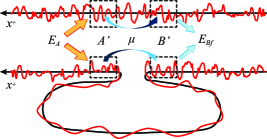
Figure 2: (Color online) Schematic showing abrupt expansion of the space where quantum fluctuation of the field becomes severely stretched. The upper figure depicts quantum fluctuation in the vacuum state before the expansion, while the lower figure depicts the stretched quantum fluctuation, which can be described by the modified mode function $v_{\omega}(x^{+})$ after the expansion.

The essence of QET without the limit of distance is as follows. The distance dependence of $E_{B}$ for vacuum-state QET comes from $C_{\mu AB}$ as defined in Eq. (5). This correlation is generated by the vacuum-state entanglement between local zero-point fluctuations in the regions of Alice and Bob. If we supply two local quantum fluctuations of $\hat{\varphi}$ that are far away from each other and with the same entanglement and correlations as those of the local zero-point fluctuations of two close regions, the QET remains effective, independent of the distance, because $C_{\mu AB}$ is the same. However, to sustain the negative-energy excitation generated by Bob, additional positive energy of the field must be placed near the negative-energy excitation. In this new protocol, the negative energy is sustained by the positive energy of the squeezed region. As depicted in Fig. 2, such a long distance correlation is indeed realized by an abrupt expansion of the space over which the quantum field $\hat{\varphi}$ exists, analogous to cosmological inflation in general relativity. The upper diagram in Fig. 2 depicts the vacuum fluctuation of $\hat{\varphi}$ in the state-preparation region, which is equipped on the right-hand side of $B$, before moving left to the original QET experimental region of $A$ and $B$. Assume that, if we perform the vacuum QET from $A^{\prime}$ to $B^{\prime}$, the distance between $A^{\prime}$ and $B^{\prime}$ in Fig. 2 is so small that the amount of teleported energy attains a large value of $E_{Bf}$. The lower diagram in Fig. 2 shows the sudden expansion of the small subspace between $A^{\prime}$ and $B^{\prime}$, which generates local excitation of $\hat{\varphi}$ due to severe stretching of the field modes. Note that the stretched mode function can be described by $v_{\omega}(x^{+})$ in a similar way to expanding Universe models including cosmological inflation KT ; BD . The expansion is specified by the metric

$$ds^{2}=g_{\mu\nu}dx^{\mu}dx^{\nu}=dt^{2}-\left(a(t,x)dx\right)^{2},$$ (21)

the scale factor of which obeys $a(t,x)=1$ outside the stretching region. Let us assume that the expansion is very rapid so that we can regard it instantaneous, and the expansion happens at time $t=0$. The initial condition of the scale factor is $a(t=-0,x)=1$, and the equation of motion of $\hat{\varphi}$ in the expansion is given by

$$\partial_{\mu}\left(\sqrt{-g}g^{\mu\nu}\partial_{\nu}\hat{\varphi}\right)=0.$$ (22)

When we consider the plane-wave mode function $u_{\omega}(x)$ in Eq. (14) just before the rapid expansion, the form of the mode function remains unchanged under the instantaneous expansion of space at the coordinate $(t,x)$. However, from Eq. (21), the correct physical distance coordinate $X$ should be obtained by

$$X=X(x)=\int_{0}^{x}a(+0,x^{\prime})dx^{\prime}.$$

Thus, the mode function after the expansion is computed in terms of the physical coordinate $(t,X)$ as

$$v_{\omega}(X)=\frac{1}{\sqrt{4\pi\omega}}e^{-i\omega x(X)},$$

where $x(X)$ is the inverse function of $X(x)$. This indeed reproduces the squeezed mode function in Eq. (13) by defining $f(X)=x(X)$. Thus, $f(x)$ in Eq. (13) is computed from the relation

$$f^{-1}(x)=\int_{0}^{x}a(+0,x^{\prime})dx^{\prime},$$

where $f^{-1}$ is the inverse function of $f$. Hence, the quantum state after the expansion is equivalent to the squeezed vacuum state given by Eq. (16). Since the field is still in a local vacuum state outside the expanded region, the correlation between $A^{\prime}$ and $B^{\prime}$ remains unchanged. Hence, if QET from $A^{\prime}$ to $B^{\prime}$ is executed, we would be able to teleport the same amount of energy $E_{Bf}$, although the distance would become very large. After the sudden expansion, the long-range correlated quantum fluctuation moves left into the experimental region including $A$ and $B$ and can be used for the original long-distance QET from $A$ to $B$ with teleported energy $E_{Bf}$.

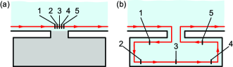
Figure 3: (Color online) Schematics of quantum Hall edge current (red lines) (a) before and (b) after the expansion.

Such spatial expansion, for example, may be performed in quantum Hall edge current systems yih . Recall that the current [red line and arrows in Fig. 3(a)] is well described by a chiral (unidirectional) massless field in one dimension yoshioka . A local extrusion of bulk electrons toward the outside [Fig. 3(b)] can be experimentally obtained by dynamically controlling the electron density in the depleted region [the gray region in Fig. 3]. Such operations are commonly used in field-effect transistors at frequencies up to the subterahertz regime. Since marked points 1–5 on the current trajectory in Fig. 3(a) are separated as in Fig. 3(b) after the extrusion, the transition describes an expansion of space in which the massless field exists. The field satisfies Eq. (22) in terms of a metric $g_{\mu\nu}$ induced by the extrusion, creating a continuously parameterized multi-mode squeezed state. Generation of such a squeezed state is well known in research of quantum fields in curved spacetime, such as inflationary universes KT , and provides an interesting squeezing method even in condensed matter physics. Finally, it should be noted that high-precision squeezed-state generation is not required for long-distance QET. However, it is imperative that a very long detour path with length $l$ for the edge current be inserted between two very-close local vacuum regions just as $A^{\prime}$ and $B^{\prime}$ in Fig. 2. This achieves the same amount of $E_{B}$ in Eq. (19). This spatial expansion method is one strategy for realizing long-distance correlation, thus facilitating experimental verification of QET and potentially contributing to quantum device applications.

V
Summary

In this paper, we have pointed out that vacuum-state QET suffers from the distance bound in Eq. (1). The bound is a severe obstacle to the implementation of long-distance QET in nanophysics. To overcome the bound on the distance $L$ between the sender and receiver of QET, we proposed a new QET protocol that adopts a squeezed vacuum state defined by Eq. (16), which corresponds to the mode function in Eq. (13) with a $C^{1}$ function $f(x)$ defined by Eqs. (9)–(12). The measurement of Alice and the local operation of Bob are the same as those of the vacuum-state QET and are given by Eqs. (2), (3), and (4). By taking an $L$-dependent squeezed state $|f\rangle$ such that the parameter $l$ of $f(x)$ satisfies Eq. (20), the long-distance damping of $E_{Bf}$ behaves as $O(L^{0})$. Therefore, QET without the limit of distance can be attained. Long-distance QET may be experimentally verified by adopting a spatial expansion method in quantum Hall edge currents, which is a new scheme to create a continuously parameterized multi-mode squeezed state in condensed matter physics.

Acknowledgments

- (1) W. Pusz and S. L. Woronowicz, Commun. Math. Phys. 58, 273 (1978).
- (2) N. D. Birrell and P. C. W. Davies, Quantum Fields in Curved Space (Cambridge Univ. Press, 1982).
- (3) H. B. G. Casimir, Proc. Kon. Nederland. Akad. Wetensch. B51, 793 (1948).
- (4) W. G. Unruh and R. M. Wald, Phys. Rev. D 29, 1047 (1984).
- (5) M. Hotta, Phys. Rev. D 78, 045006 (2008).
- (6) M. Hotta, Phys. Rev. D 81, 044025 (2010).
- (7) C. H. Bennett, G. Brassard, C. Crépeau, R. Jozsa, A. Peres, and W. K. Wootters, Phys. Rev. Lett. 70, 1895 (1993).
- (8) M. R. Frey, K. Gerlach, and M. Hotta, J. Phys. A: Math. Theor. 46, 455304 (2013).
- (9) M. Hotta, Phys. Lett. A 372, 5671 (2008).
- (10) Y. Nambu and M. Hotta, Phys. Rev. A 82, 042329 (2010).
- (11) M. Hotta, Phys. Rev. A 80, 042323 (2009).
- (12) G. Yusa, W. Izumida, and M. Hotta, Phys. Rev. A 84, 032336 (2011).
- (13) D. Yoshioka, The Quantum Hall Effect (Springer, Berlin, 2002).
- (14) For information on general measurement, see M. A. Nielsen and I. L. Chuang, Quantum Computation and Quantum Information, (Cambridge Univ. Press, 2000) p. 90.
- (15) For example, a general measurement using a nanoscale RC circuit has been proposed as a realistic QET experiment in quantum Hall edge currents yih .
- (16) E. E. Flanagan, Phys. Rev. D 56, 4922 (1997).
- (17) E. W. Kolb and M. S. Turner, The Early Universe (Addison-Wesley, 1990).