MHD Disc Winds and Line Width Distributions

Abstract

We study AGN emission line profiles combining an improved version of the accretion disc-wind model of Murray & Chiang with the magneto-hydrodynamic model of Emmering et al. We show how the shape, broadening and shift of the C iv ​ line depend not only on the viewing angle to the object but also on the wind launching angle, especially for small launching angles. We have compared the dispersions in our model C iv ​ linewidth distributions to observational upper limit on that dispersion, considering both smooth and clumpy torus models. As the torus half-opening angle (measured from the polar axis) increases above about 18°, increasingly larger wind launching angles are required to match the observational constraints. Above a half-opening angle of about 47°, no wind launch angle (within the maximum allowed by the MHD solutions) can match the observations. Considering a model that replaces the torus by a warped disc yields the same constraints obtained with the two other models.

1 Introduction

Broad Emission Lines (BELs) are one characteristic feature of the spectra of Type 1 Active Galactic Nuclei (AGNs). Lines arising from high-ionization species are generally blueshifted and single-peaked (e.g. Sulentic et al., 1995, 2000; Vanden Berk et al., 2001). Quasars (and AGN in general) are powered by accreting mass into a central super-massive black hole (SMBH). The accreting mass is assumed to form a disc-like structure, responsible for most of the ultraviolet (UV) and optical continuum emission. This continuum emission illuminates and ionizes dense gas surrounding the central engine and forms the Broad Line Region (BLR), where the BELs originate. The black hole, disc and BLR are embedded in a dusty toroidal structure that obscures some lines of sight to the nucleus (e.g., Elitzur, 2008). In the model of Lawrence & Elvis (2010), the torus is replaced by a warped disc.

Currently there is no consensus on the nature of the BLR and numerous models have been developed to explain it. The spectroscopic characteristics of the BEL can be explained by lines arising from either an approximately spherical distribution of discrete clouds, with no preferred velocity direction (e.g., Kaspi & Netzer, 1999) or at the base of a wind from an accretion disc (e.g., Murray et al., 1995; Murray & Chiang, 1997; Bottorff et al., 1997). In the cloud scenario, the BLR is described as composed of numerous optically-thick clouds that, photoionized by the continuum-source emission, are the emitting entities responsible for the observed lines. Although this model can explain many observed spectral features, it also leaves several unsolved issues, such as the formation and confinement of the clouds (e.g., Netzer, 1990). The two relevant time-scales for these clouds are the sound crossing time $t_{\mathrm{sc}}$ and the dynamical time $t_{\mathrm{dyn}}$. According to the models, the masses of individual BLR clouds are below their Jeans mass, therefore without a confinement mechanism such clouds will disintegrate on a time-scale $t_{\mathrm{sc}}\ll t_{\mathrm{dyn}}$, in which case they would need to be continuously produced. In addition, the number of clouds needed to reproduce the observed smoothness of BEL profiles (Arav et al., 1998; Dietrich et al., 1999) is implausibly large. Furthermore, even if the clouds are confined, cloud-cloud collisions would destroy the clouds on a dynamical timescale (e.g. Mathews & Capriotti, 1985), again requiring a high rate of cloud formation or injection.

One approach aimed at solving the discrete-cloud model difficulties was proposed by Emmering, Blandford & Shlosman (1992). In their model, the BLR is associated with disc-driven, hydromagnetic winds and the lines are formed by clouds which are confined by the magnetic pressure. Low-ionization line profiles, (e.g., Mg ii), and high-ionization line profiles (e.g., C iv) are produced in the wind at different latitudes and radii. Within that framework, the estimated values of parameters such as ionizing flux, electron density, cloud filling factor, column density, and velocity are in agreement with values for these quantities inferred from observations. Emmering et al. (1992) consider emission models with and without electron scattering and attempt to construct a typical C iv  emission profile. Different blueshifts and line asymmetries are obtained by varying model parameters.

Murray et al. (1995) and later Murray & Chiang (1997, 1998) proposed a wind model motivated by the similarities between broad emission lines in AGNs and other astrophysical objects, such as cataclysmic variables, protostars and X-ray binaries. They made the assumption that the outflow is continuous instead of being composed of discrete clouds and showed that such a continuous, optically thick, radiatively driven wind launched from just above the accretion disc can account for both the single-peaked nature of AGN emission lines and their blueshifts with respect to the AGN systemic redshift, although not for the magnitude of these shifts. In a accelerating wind, the wind opacity in a given direction depends on the velocity gradient in that direction. The larger radial gradient of velocity in a radially accelerating wind means that the opacity seen by radially-emitted photons will be lower than the opacity seen by photons emitted in other directions. Thus, photons will tend to escape radially and the resultant emission lines are single-peaked. In addition, the model high-velocity component of the wind naturally explains the existence of blueshifted broad absorption lines seen in an optically selected subset (15-20$\%$) of the quasar population, known as broad absorption line quasars.

Here we combine an improved version of the Murray & Chiang (1997) model with the Emmering et al. (1992) model and analyse the dependence of the resulting emission line profiles on several parameters. The plan of the paper is as follows. In Section 2 we review the Murray & Chiang (1997) disc-wind model and the modifications that we have introduced in a companion paper (Hall et al., in preparation). In Section 3 we outline the basics of MHD winds and show how we combined the two models. In section  4 we calculate a key quantity of the model, $Q$: the line-of-sight gradient of the line-of-sight velocity. The line profile results are presented in Section 5. In Section 6 we follow Fine et al. (2008) and study the predicted BEL width distribution incorporating two models for the escape probability from the BLR, including the clumpy torus model of Nenkova et al. (2008a, 2008b), and use the results to obtain constraints on the torus parameters. We analyse the warped disc models of Lawrence & Elvis (2010) in a similar fashion in Section 7. We present our conclusions in Section 8.

2 The Modified Wind Model

In a companion paper (Hall et al. 2012, in preparation) we extend the disc-wind model of Murray & Chiang (1997, MC97 hereafter) to the case of non-negligible radial and vertical velocities. The new treatment retains a number of factors neglected in MC97 and introduces the ‘local inclination angle’ to account for the different effective inclinations to the line of sight of different portions of the emitting region. Below we summarize these modifications.

As shown in Figure 1, we assume the SMBH is at the origin of a cylindrical coordinate system ($r,\phi,z$) with the $z$ axis normal to the accretion disc and the observer, in the $xz$ plane, making an angle $i$ with the disc axis. At any $r$, the azimuthally symmetric emitting region has its base at $z_{\mathrm{em}}=r\tan\beta(r)$ above the disc plane and has a density which drops off above the base as a Gaussian with characteristic thickness that satisfies $l_{\mathrm{em}}(r)\ll r$. Because the photons originate in a narrow layer above the disk, the emission region can be approximated as an emitting surface with a source function $S_{\nu}$ that is a function of radius only. The wind streamlines make an angle of $\vartheta(r,z)$ relative to the disc plane.

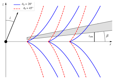
Figure 1: Streamlines for two different launching angles: $\vartheta_{0}=20\degr,45\degr$. The blue line represents the base of the emitting region, tilted by an angle $\beta$ with respect to the disc plane.

Under these assumptions, the specific luminosity for a given line in the direction of the observer, $L_{\nu}({\bf\hat{n}})$, is given by

$$L_{\nu}({\bf\hat{n}})=\int_{r_{\mathrm{min}}}^{r_{\mathrm{max}}}\!\!\!\!\!\!\!\!\!\!\!\!\!S_{\nu}(r)~{}a(r)~{}r~{}dr\int_{0}^{2\pi}\!\!\!\!\!\![1-e^{-\tau_{\nu}(r,\phi,{\bf\hat{n}})}]\cos\iota(r,\phi,{\bf\hat{n}})~{}d\phi$$ (1)

where $I_{\nu}=S_{\nu}(r)[1-e^{-\tau_{\nu}}]$ is the specific intensity, $a(r)~{}r~{}dr~{}d\phi$ is the area of the emitting surface between cylindrical radii $r$ and $r+dr$, $\tau_{\nu}$ is the optical depth from $z_{\mathrm{em}}(r)=r\tan\beta(r)$ to infinity along the direction $\bf{\hat{n}}$ from the location $(r,\phi)$, and $\iota(r,\phi,{\bf\hat{n}})$ is the local inclination angle between ${\bf\hat{n}}$ and the local normal to the surface at radius $r$ and azimuthal angle $\phi$. For $i<90\degr-\beta(r)$, the area factor and the local inclination angle are given by

$$a(r)=\frac{1}{\cos\beta(r)}$$ (2)

and

$$\cos\iota=\cos i\cos\beta(r)-\cos\phi\sin i\sin\beta(r)\,,$$ (3)

respectively.

To evaluate the optical depth $\tau_{\nu}$, MC97 expanded the projection of the wind velocity along the line of sight, $\mathbf{\vec{v}\cdot\hat{n}}$, in terms of $z-z_{\mathrm{em}}$ to first order to obtain (their equation 12)

$$\mathbf{\hat{n}\cdot\vec{v}}(r,\phi,z) \cong\mathbf{\hat{n}\cdot\vec{v}}(r,\phi,z_{\mathrm{em}})+\mathbf{\hat{n}\cdot\Lambda\cdot\hat{n}}~{}\frac{(z-z_{\mathrm{em}})}{\cos\iota/\cos\beta}$$

$$\equiv v_{\mathrm{D}}(r,\phi,z_{\mathrm{em}})+\frac{(z-z_{\mathrm{em}})}{l_{\mathrm{em}}}~{}v_{\mathrm{sh}}(r,\phi,z_{\mathrm{em}}).$$ (4)

The zeroth order term in Equation 2 is the Doppler velocity $v_{\mathrm{D}}$:

$$v_{\mathrm{D}}=-v_{\phi}\sin\phi\sin i+v_{\mathrm{p}}\left(\cos\phi\cos\vartheta\sin i+\sin\vartheta\cos i\right)$$ (5)

where $v_{\phi}$ and $v_{\mathrm{p}}$ are, respectively, the azimuthal and poloidal velocities of the wind at $z=z_{\mathrm{em}}$.

The first order term in Equation 2 involves the shear velocity $v_{\mathrm{sh}}$, defined as $v_{\mathrm{sh}}=l_{\mathrm{em}}Q\cos\beta/\cos\iota$ where $Q$ (Rybicki & Hummer, 1978, 1983) is the line-of-sight gradient of the line-of-sight wind velocity:

$$Q\equiv\mathbf{\hat{n}\cdot\Lambda\cdot\hat{n}}$$ (6)

where $\mathbf{\hat{n}}$ is the unit vector in the line of sight direction and $\mathbf{\Lambda}$ is the strain tensor. The entries of the strain tensor $\Lambda$ consist of spatial derivatives of velocity components. It is symmetric ($\Lambda_{ij}=\Lambda_{ji}$) and its elements are given in cylindrical coordinates by (see e.g. Batchelor, 1967):

$$\Lambda_{r\phi} =\frac{1}{2}\left(\frac{1}{r}\frac{\partial v_{r}}{\partial\phi}-\frac{v_{\phi}}{r}+\frac{\partial v_{\phi}}{\partial r}\right),\quad\Lambda_{rz}=\frac{1}{2}\left(\frac{\partial v_{r}}{\partial z}+\frac{\partial v_{z}}{\partial r}\right),$$

$$\Lambda_{\phi z} =\frac{1}{2}\left(\frac{\partial v_{\phi}}{\partial z}+\frac{1}{r}\frac{\partial v_{z}}{\partial\phi}\right),$$

$$\Lambda_{rr} =\frac{\partial v_{r}}{\partial r},\quad\Lambda_{\phi\phi}=\frac{1}{r}\frac{\partial v_{\phi}}{\partial\phi}+\frac{v_{r}}{r},\quad\Lambda_{zz}=\frac{\partial v_{z}}{\partial z}.$$ (7)

In terms of these $\Lambda_{ji}$, the quantity $Q$ is:

$$\begin{split}Q&=\sin^{2}i\left[\Lambda_{rr}\cos^{2}\phi+\Lambda_{\phi\phi}\sin^{2}\phi-2\Lambda_{r\phi}\sin\phi\cos\phi\right]+\\ &\quad\cos i\left[2\Lambda_{rz}\sin i\cos\phi+\Lambda_{zz}\cos i-2\Lambda_{\phi z}\sin i\sin\phi\right]\\ \end{split}$$ (8)

Assuming azimuthal symmetry, all the $\partial/\partial\phi=0$ and the simplified expressions for the different $\Lambda_{ij}$ are:

$$\Lambda_{r\phi} =\frac{1}{2}\left(\frac{\partial v_{\phi}}{\partial r}-\frac{v_{\phi}}{r}\right),\quad\Lambda_{rz}=\frac{1}{2}\left(\frac{\partial v_{r}}{\partial z}+\frac{\partial v_{z}}{\partial r}\right),$$

$$\Lambda_{\phi z} =\frac{1}{2}\frac{\partial v_{\phi}}{\partial z},\quad\Lambda_{rr}=\frac{\partial v_{r}}{\partial r},\quad\Lambda_{\phi\phi}=\frac{v_{r}}{r},\quad\Lambda_{zz}=\frac{\partial v_{z}}{\partial z}$$ (9)

In the above, the novel element introduced in Hall et al. (2012, in preparation) is the dropping of the assumption of $v_{r}\ll v_{\phi}$, thus allowing for non-negligible radial and vertical velocities.

Including that and several factors that have been omitted or considered negligible in the original MC97 work, the final expression for the specific luminosity in a line of central frequency $\nu_{0}$ emitted from a disc with a disc wind is given by

$$\begin{split}L_{\nu}(i)&=\int_{r_{\mathrm{min}}}^{r_{\mathrm{max}}}S_{\nu}(r)~{}a(r)~{}r~{}dr\int_{0}^{2\pi}\cos\iota(r,\phi,i)~{}\times\\ &(1-\exp[-\tau(r,\phi,i)\times e_{\nu}(r,\phi,i)\times e^{-x_{\nu}^{2}(r,\phi,i)}])~{}d\phi\end{split}$$ (10)

where

$$\tau(r,\phi,i)\equiv\frac{ck_{0}(r)/2\nu_{0}}{\sqrt{Q^{2}(r,\phi,i)+q_{\mathrm{tt}}^{2}(r,\phi,i)}}$$ (11)

$$e_{\nu}(r,\phi,i)\equiv{\mathrm{\,erfc}}\left(-\frac{\nu-\nu_{\mathrm{D}}(r,\phi,i)}{\sqrt{2}\Delta\nu_{\mathrm{tt}}\sqrt{1+q_{\mathrm{tt}}^{2}(r,\phi,i)/Q^{2}(r,\phi,i)}}\right)\\$$ (12)

$$x_{\nu}^{2}(r,\phi,i)\equiv\frac{1}{2}\left(\frac{\nu-\nu_{\mathrm{D}}(r,\phi,i)}{\Delta\nu_{\mathrm{tt}}\sqrt{1+Q^{2}(r,\phi,i)/q^{2}_{\mathrm{tt}}(r,\phi,i)}}\right)^{2}$$ (13)

and erfc is the complementary error function. In the above expression, the $k_{0}(r)$ is the integrated line opacity (units of Hz/cm) at $z_{\mathrm{em}}$, and we have defined the Doppler-shifted central frequency of the line emitted towards the observer from location ($r,\phi$) on the emitting surface, $\nu_{\mathrm{D}}=\nu_{0}(1+v_{\mathrm{D}}/c)$, and the ‘thermal $Q$’, the ratio of the characteristic thermal plus turbulent velocity of the ion to the thickness of the emitting layer along the line of sight, $q_{\mathrm{tt}}(r,\phi,i)=v_{\mathrm{tt}}\cos\iota(r,\phi,i)/l_{\mathrm{em}}(r)\cos\beta(r)$, with $v_{\mathrm{tt}}^{2}\equiv v_{\mathrm{th}}^{2}+v_{\mathrm{turb}}^{2}$. The effective frequency dispersion of the line is given by $\Delta\nu_{\mathrm{tt}}=\nu_{0}v_{\mathrm{tt}}/c$. The $z$-dependent quantities are evaluated at $z=z_{\mathrm{em}}$ where applicable. The emission region thickness is given by

$$l_{\mathrm{em}}(r)=0.1{z_{\mathrm{em}}}\left[{v_{\mathrm{tt}}+v_{\mathrm{p}}(r,z_{\mathrm{em}})\over v_{\mathrm{tt}}+v_{\infty}(r,z_{\mathrm{em}})}\right].$$ (14)

3 Magneto-hydrodynamic wind model

The presence of an ordered magnetic field threading an AGN accretion disc has been suggested by several authors (e.g., Blandford & Payne, 1982; Contopoulos & Lovelace, 1994; Königl & Kartje, 1994) as a mechanism able to either confine the clouds (as in Emmering et al., 1992) or direct the outflow velocity field (e.g., Everett, 2005). Along with most works in the field, we do not discuss here the origin of the magnetic field, but assume it is present and study its effects within the postulated framework.

The standard magneto-hydrodynamic (MHD) wind equations are:

$$\frac{\partial\rho}{\partial t}+\mathbf{\nabla}\cdot(\rho\mathbf{v}) =0$$ (15a)

$$\rho\frac{\partial\mathbf{v}}{\partial t}+\rho(\mathbf{v}\cdot\mathbf{\nabla})\mathbf{v} =-\mathbf{\nabla}p-\rho\mathbf{\nabla}\Phi_{\mathrm{g}}+\frac{1}{4\pi}(\mathbf{\nabla}\times\mathbf{B})\times\mathbf{B}$$ (15b)

$$\frac{\partial\mathbf{B}}{\partial t} =\mathbf{\nabla}\times(\mathbf{v}\times\mathbf{B})$$ (15c)

$$\mathbf{\nabla}\cdot\mathbf{B} =0,$$ (15d)

where $\mathbf{B}$ and $\mathbf{v}$ are respectively the magnetic and velocity fields, $\rho$ is the mass density, $p$ is the thermal pressure and $\Phi_{\mathrm{g}}$ is the gravitational potential.

We look for steady state wind solutions for this model. In that case (i.e. when $\partial/\partial t=0$), there are conserved quantities along each magnetic field line (e.g., Mestel, 1968), such as

mass to magnetic flux ratio,

$$\frac{k}{4\pi}=\frac{\rho v_{\mathrm{p}}}{B_{\mathrm{p}}}$$ (16)

specific angular momentum,

$$l=r\left(v_{\phi}-\frac{B_{\phi}}{k}\right)\\$$ (17)

specific energy

$$e=\frac{v^{2}}{2}+h+\Phi_{\mathrm{g}}-\frac{r\Omega B_{\phi}}{k}$$ (18)

where $h$ is the specific enthalpy, and, owing to the axisymmetry of the problem, we have separated the velocity and magnetic fields into their poloidal and azimuthal components:

$$\mathbf{v}=\mathbf{v}_{p}+\mathbf{v}_{\phi}\;\;\qquad\qquad\hfill\mathbf{B}=\mathbf{B}_{p}+\mathbf{B}_{\phi}$$ (19)

3.1 Self-similar solutions

Solutions of the steady, axisymmetric, non-relativistic ideal MHD equations assuming a spherically self-similar scaling were obtained by e.g. Blandford & Payne (1982, BP82 hereafter) for the cold plasma outflow from the surface of a Keplerian disc. This solution for the field can be written in terms of variables $\chi$, $\xi(\chi)$, $\phi$, and $r_{0}$, which are related to the cylindrical coordinates via

$$\mathbf{r}\equiv\left[r,\phi,z\right]=\left[r_{0}\xi(\chi),\phi,r_{0}\chi\right],$$ (20)

where the adopted independent variables $(r_{0},\chi)$ are a pair of spatial coordinates analogous to $(r,z)$. The function $\xi(\chi)$ describes the shape of the field lines and, in the general case, is not a priori known, but found as part of a self-consistent solution to the MHD equations. The flow velocity components are given by

$$\mathbf{v}=\left[\xi^{\prime}(\chi)f(\chi),g(\chi),f(\chi)\right]\sqrt{\frac{GM}{r_{0}}},$$ (21)

where a prime denotes differentiation with respect to $\chi$, and $G$ and $M$ are respectively the gravitational constant and the mass of the central black hole.

In this self-similar model, the scaling of the speed $v$, magnetic field amplitude $B$, and gas density $\rho$ with the spherical radial coordinate $r$ is determined from the relation $B/\sqrt{\rho}\propto r^{-1/2}$ and from the assumption that $r_{0}^{2}\rho v_{0}$ is independent of $r_{0}$, from where $\rho_{0}\propto r_{0}^{-3/2}$ and $B_{0}\propto r_{0}^{-5/4}$. Other authors (e.g., Contopoulos & Lovelace, 1994; Emmering et al., 1992) generalized this class of self-similar solutions by considering winds with a density scaling $\rho\propto r^{-b}$, for which $B\propto r^{-(b+1)/2}$. Note that, in this context, the BP82 solution corresponds to $b=3/2$. The magnetic field and density at arbitrary positions can be then written, in accordance with the self-similarity Ansatz (20), as ${\bf{B}}=B_{0}(r_{0}){\bf{b}}(\chi)$ and $\rho=\rho_{0}(r_{0})\varrho(\chi)$. On the disc plane the rotational velocity, $v_{\phi}$, is Keplerian and scales as $v_{\phi}\propto r_{0}^{-1/2}$. The functions $\xi(\chi)$, $f(\chi)$ and $g(\chi)$ have to satisfy the flow MHD equations subject to the above scalings of $\rho$, $B$, and $v_{\phi}$ and boundary conditions. In particular, at the disc surface $\xi(0)=1$, $f(0)=0$ and $g(0)=1$.

Following BP82, we introduce the dimensionless expressions of the integrals of motion defined in equations 16-18, in terms of which the solutions are defined:

$$\kappa=k(1+\xi^{\prime}_{0})^{1/2}\frac{(GM/r_{0})^{1/2}}{B_{0}}$$ (22)

$$\lambda=\frac{l}{(GMr_{0})^{1/2}}\\$$ (23)

$$\epsilon=\frac{e}{(GM/r_{0})}$$ (24)

The parameters of the model are $\epsilon$, $\lambda$ and $\kappa$ and $\xi^{\prime}_{0}$. However, due to the regularity conditions that must be satisfied, these parameters are not independent. Combining equations 23 and 24 gives $\epsilon~{}=~{}\lambda-\frac{3}{2}$. The value of $\xi^{\prime}_{0}\equiv\xi^{\prime}(\chi=0)$ must be chosen to ensure the regularity of the solution at the Alfvén point. The solutions are therefore parametrized only by two numbers, which can be chosen to be $\kappa$ and $\lambda$ (e.g. BP82).

The Alfvén speed, $v_{\mathrm{A}}$, is the characteristic velocity of the propagation of magnetic signals in an MHD fluid and is defined by:

$$v_{\mathrm{A}}=\frac{B^{2}}{\mu_{0}\,\rho},$$ (25)

where $\mu_{0}$ is the vacuum permeability. Another important characteristic quantity in magnetized fluids is the Alfvén Mach number at each position. The square of this quantity is expressed in the present model as

$$m(\chi)=\frac{v_{\mathrm{p}}^{2}}{v_{\mathrm{pA}}^{2}}=\frac{4\pi\rho\,v_{\mathrm{p}}^{2}}{B_{\mathrm{p}}^{2}}=\kappa\,f(\chi)\,\xi(\chi)\,J(\chi),$$ (26)

where

$$J(\chi)=\xi(\chi)-\chi\;\xi^{\prime}(\chi)$$ (27)

is the determinant of the Jacobian matrix of the transformation $(r,z)\rightarrow(r_{0},\chi)$ and $v_{\mathrm{pA}}$ is the poloidal component of the Alfvén velocity.

The function $g(\chi)$ can be expressed in terms of the function $m$ and the specific angular momentum, $\lambda$:

$$g(\chi)=\frac{\xi^{2}(\chi)-\lambda\,m(\chi)}{\xi(\chi)\left[1-m(\chi)\right]}.$$ (28)

From this expression we can see that the point corresponding to $m=1$ is a singular point of the problem. In particular, to avoid unphysical solutions there, we must have $\xi_{\mathrm{A}}=\xi(\chi_{\mathrm{A}})=\lambda^{1/2}$, where the subscript A refers to the Alfvén point.

Expressing $f$ and $g$ by Eqs (26) and (28) in terms of the Alfvénic Mach number and of the function $\xi(\chi)$ and its derivatives, Eq. (18) is transformed into a fourth degree equation for the function $f(\chi)$:

$$T-f^{2}(1+\xi^{\prime 2})=\left[\frac{(\lambda-\xi^{2})\,m}{\xi(1-m)}\right]^{2},$$ (29)

where

$$T=\xi^{2}+\frac{2}{\sqrt{\xi^{2}+\chi^{2}}}-3.$$ (30)

Using the differential form of equation 29 combined with the $z$-component of the momentum equation (Eq. 15b), BP82 obtain a second-order differential equation for $\xi(\chi)$. The flow is then fully specified by that equation and equation 29, plus the boundary conditions, $\xi(0)=1$ and $\xi^{\prime}(0)=\xi^{\prime}_{0}$.

The model of Emmering et al. (1992, hereafter EBS92) represents a simplified version of BP82 solution. The EBS92 solution corresponds to the case in which the solution asymptotically approaches $n=1$ as $\chi\rightarrow\infty$, where $n$ is the square of the Mach number for the fast magnetosonic mode for an arbitrary scaling of density $\rho_{0}\propto r_{0}^{-b}$ and magnetic field $B_{0}\propto r_{0}^{-(b+1)/2}$. The quantity $n$ is given by (e.g. BP82, BPS92):

$$n=\frac{4\pi\rho\,v_{\mathrm{p}}^{2}}{B^{2}}=\frac{\kappa\,\xi\,f^{3}J(1+\xi^{\prime 2})}{T}.$$ (31)

While BP82 found their solutions by integrating a second-order differential equation, EBS92 impose a priori the functional form of the solution so that it will asymptotically tend to the BP82 solution. In their equation (3.19), EBS92 give an explicit form for the function $\xi(\chi)$:

$$\xi=\left(\frac{\chi}{c_{2}}+1\right)^{1/2},$$ (32)

where $c_{2}=\frac{1}{2}\tan\vartheta_{0}$ was chosen to ensure that the field lines make an initial angle $\vartheta_{0}$ with the disc plane, so that $\cot\vartheta_{0}=\xi^{\prime}_{0}$ and the subscript $0$ means that the quantities are evaluated at the disc plane. It can be demonstrated (e.g. BP82, Heyvaerts, 1996) that there is an upper limit for this angle: $\vartheta_{0}<60\degr$.

EBS92 found that to satisfy the condition that $n\rightarrow 1$ when $\chi\rightarrow\infty$, the parameters $\kappa$ and $\lambda$ must be related by:

$$\kappa=2\left(\frac{3}{2\lambda-3}\right)^{3/2}$$ (33)

In addition, the asymptotic value of the function $f$ is given by

$$f_{\infty}=\left(\frac{2\lambda-3}{3}\right)^{1/2}.$$ (34)

Thus, in this model the solutions depend on $\lambda$ and $\vartheta_{0}$. Figure 1 depicts the streamlines for two different launching angles.

Note that in the general case, in order to find the flow variables, we should have solved a second-order differential equation $\xi^{\prime\prime}=\xi^{\prime\prime}(\chi,\xi,\xi^{\prime},f(\chi))$, with $f(\chi)$ given implicitly by equation 29. However, by using the EBS92 model we could evaluate $f^{\prime}$, $m$ and $g^{\prime}$ from an analytic estimate for $f$. The point of having used an analytical functional form for $f(\chi)$ has to do with the inclusion of the velocity field in the MC97 model. The opacity depends on the projection of the line of sight (LOS) component of the gradient of the LOS velocity through the quantity $Q$ (equation 8), which involves the spatial derivatives of velocity components. Combining the EBS92 functional form for $\xi(\chi)$ and $\xi_{\mathrm{A}}=\lambda^{0.5}$ it is straightforward to obtain $\chi_{\mathrm{A}}=(\lambda-1)c_{2}$. In the general case this quantity must be found numerically as part of the solution. However, in the adopted framework, all related quantities at the Alfvén point are easily found (because $m_{\mathrm{A}}\equiv m(\chi_{\mathrm{A}})=1$ ). In particular,

$$f_{\mathrm{A}}=\frac{1}{\kappa\sqrt{\lambda}J_{\mathrm{A}}}=\frac{1}{\kappa\sqrt{\lambda}[\xi(\chi_{\mathrm{A}})-\chi_{\mathrm{A}}\xi^{\prime}(\chi_{\mathrm{A}})]}.$$ (35)

The derivative of $f(\chi)$ at $\chi=0$, $f^{\prime}(\chi=0)=f^{\prime}_{0}$, is given by BP82 (their equation 2.23c), reproduced here:

$$f^{\prime}_{0}=\frac{(3\xi^{\prime 2}_{0}-1)^{1/2}}{\kappa^{2}\left[(\lambda-1)^{2}+(1+\xi^{\prime 2}_{0})\right]^{1/2}}\;.$$ (36)

We thus adopt

$$f(\chi)=f_{\infty}\frac{e^{k_{1}\chi}-1}{e^{k_{1}\chi}+k_{2}}\;$$ (37)

and look for $k_{1}$ and $k_{2}$ such that the conditions for $f_{\mathrm{A}}$ and $f^{\prime}_{0}$ are satisfied. Once $f(\chi)$ is found, $m(\chi)$ and thus $g(\chi)$ are obtained. We then have the three wind velocity components expressed in analytical form.

Note that, as already mentioned, EBS92 model postulates that the emission lines arise in clouds confined by an MHD flow. However, we follow MC97 and Murray & Chiang (1998, MC98 hereafter) in assuming that the lines form in a continuous medium. As will be discussed in section 5, we consider line emissivity obtained by CLOUDY photoionization model, different from either of the emissivity laws adopted by EBS92. Two of those emissivity models include electron scattering, which is not considered in our model. In EBS92 the dimensionless angular momentum $\lambda$ and the launch angle are fixed, while in our work the former is still fixed but the latter is varied to study its effect on the profiles. It is important to note that, while EBS92 obtains the line luminosity integrating in the two poloidal variables, we include the $z$-integral in the optical depth expression.

4 Determination of $Q$ for self-similar MHD winds

For self-similar solutions of MHD winds, the derivatives needed to obtain the different $\Lambda_{ij}$ that appear in the quantity $Q$ have to be evaluated using the rules for changing variables (e.g., Königl, 1989)

$$\frac{\partial}{\partial r}=\frac{1}{J}\frac{\partial}{\partial r_{0}}-\frac{\chi}{r_{0}J}\frac{\partial}{\partial\chi},$$ (38)

$$\frac{\partial}{\partial z}=-\frac{\xi^{\prime}}{J}\frac{\partial}{\partial r_{0}}+\frac{\xi}{r_{0}J}\frac{\partial}{\partial\chi},$$ (39)

where $J(\chi)$ has been defined in Eq. (27). Thus, we have the following expressions, where for clarity we omit the functional dependence of the dependent variables:

$$\Lambda_{rr}=-\frac{1}{J}\sqrt{\frac{GM}{r_{0}^{3}}}\;\left(\frac{\xi^{\prime}f}{2}+\chi\left(\xi^{\prime\prime}f+\xi^{\prime}f^{\prime}\right)\right)$$ (40)

$$\Lambda_{\phi\phi}=\sqrt{\frac{GM}{r_{0}^{3}}}\;\frac{\xi^{\prime}f}{\xi}$$ (41)

$$\Lambda_{zz}=\frac{1}{J}\sqrt{\frac{GM}{r_{0}^{3}}}\;\left(\frac{\xi^{\prime}f}{2}+\xi f^{\prime}\right)$$ (42)

$$\Lambda_{rz}=\frac{1}{2J}\sqrt{\frac{GM}{r_{0}^{3}}}\left[\left(\frac{\xi^{\prime 2}}{2}+\xi\xi^{\prime\prime}-\frac{1}{2}\right)\,\!f+\left(\xi\xi^{\prime}-\chi\right)\,\!f^{\prime}\right]$$ (43)

$$\Lambda_{r\phi}=\frac{1}{2}\;\sqrt{\frac{GM}{r_{0}^{3}}}\left[-\frac{1}{J}\left(\frac{g}{2}+\chi g^{\prime}\right)+\frac{g}{\xi}\right]$$ (44)

$$\Lambda_{\phi z}=\frac{1}{2J}\;\sqrt{\frac{GM}{r_{0}^{3}}}\left(\frac{\xi^{\prime}g}{2}+\xi g^{\prime}\right)$$ (45)

For the particular form of $\xi(\chi)$ given by EBS92 the corresponding expressions for the strain tensor entries are:

$$\Lambda_{rr}=-\sqrt{\frac{GM}{r_{0}^{3}}}\;\left[\frac{fc_{2}+2\chi^{2}f^{\prime}+2\chi f^{\prime}c_{2}}{2\left(\chi+c_{2}\right)\left(\chi+2c_{2}\right)}\right]$$ (46)

$$\Lambda_{\phi\phi}=\sqrt{\frac{GM}{r_{0}^{3}}}\;\left[\frac{f}{2(\chi+c_{2})}\right]$$ (47)

$$\Lambda_{zz}=\sqrt{\frac{GM}{r_{0}^{3}}}\;\left[\frac{f+4f^{\prime}\left(\chi+c_{2}\right)}{2(\chi+2c_{2})}\right]$$ (48)

$$\Lambda_{rz}\!=\!\sqrt{\frac{GM}{r_{0}^{3}}}\!\left[\frac{4\left(\chi+c_{2}-2c_{2}\chi^{2}-2c_{2}^{2}\chi\right)\!\!f^{\prime}\!-\!\left(1+4c_{2}\chi+4c_{2}^{2}\right)f}{8\sqrt{c_{2}}\left(\chi+2c_{2}\right)\sqrt{\chi+c_{2}}}\right]$$ (49)

$$\Lambda_{r\phi}=-\sqrt{\frac{GM}{r_{0}^{3}}}\sqrt{c_{2}}\left[\frac{(2\chi+3c_{2})g+2\chi(\chi+c_{2})g^{\prime}}{2\left(\chi+2c_{2}\right)\sqrt{\chi+c_{2}}}\right]$$ (50)

$$\Lambda_{\phi z}=-\sqrt{\frac{GM}{r_{0}^{3}}}\left[\frac{g+4g^{\prime}\chi+4g^{\prime}c_{2}}{4\left(\chi+2c_{2}\right)}\right]$$ (51)

5 Line Profiles

We evaluated the line luminosity (Eq. 10) using the EBS92 solution to estimate the quantities included there and in the associated equations 11 and 13. In summary, $v_{\mathrm{D}}$ and $Q$ are computed as functions of position ($r,\phi,z$) from the velocity field given by the EBS92 model. Then, these two quantities and the ‘thermal $Q$’, $q_{\mathrm{tt}}$, are used to evaluate the optical depth $\tau(r,\phi,i)$ (Eq. 11) and the quantities $e_{\nu}(r,\phi,i)$ (Eq. 12) $x_{\nu}(r,\phi,i)$ (Eq. 13). We emphasize again that the integral in the $z$ direction is included in the optical depth expression. We then calculate $L_{\nu}({\bf\hat{n}})$ by integrating over all ($r,\phi$) (Eq. 10). The process is repeated for different $\nu$ values to build up the profile of the given emission line for the given input parameters.

We have computed the C iv  line profile for different combinations of inclination angle, $i$ and initial angle, $\vartheta_{0}$. We also studied the results of changing the initial density and the exponent of the power law that governs the radial behaviour of the density. The specific luminosity from each component of the C iv  doublet is computed separately, and then the results added together. In Table 1 we list the meaning and adopted values of the main parameters in the model. The fiducial values adopted for the density, density power-law exponent and thermal plus turbulent velocity are $n_{0}=10^{11}$ cm^-3, $b=2$ and $v_{\rm tt}=10^{7}$ cm s^-1, respectively.

We determine the source function for our simulations by applying the reverberation mapping results of Kaspi et al. (2007) to the radial line luminosity function $L(r)$ calculated by MC98 for a quasar with $L_{1350}\equiv\nu L_{\nu}(1350~{}{\mathrm{\AA}})=10^{46}$ erg s^-1 and shown in their Figure 5b. According to that figure, the peak C iv  emission is reached at $R_{CIV}=10^{18}$ cm, but the Kaspi et al. (2007) results show that $R_{CIV}$ is smaller for a quasar of that luminosity. Their Equation 3 gives

$$R_{CIV}=6.216\times 10^{15}{\rm~{}cm}\left({L_{1350}\over 10^{43}{\rm~{}erg\,s}^{-1}}\right)^{\alpha},$$ (52)

where $\alpha=0.55\pm 0.04$ in the original formulation and for simplicity we have adopted $\alpha=0.5$. Eq. 52 gives $R_{CIV}=2\times 10^{17}$ cm for a quasar with $L_{1350}=10^{46}$ erg s^-1. We therefore empirically adjust all the radii in the MC98 Figure 5b line luminosity function down by a factor of five. Each point in the line luminosity function now gives the line luminosity $L(r_{i})$ in a logarithmic bin spanning a factor of $\sqrt{10}$ in radius centred on adjusted radius $r_{i}$ for a quasar with $L_{1350}=10^{46}$ erg s^-1.

Table 1: Set of parameters used in the simulation.

Variable	Value	Explanation
$M_{\mathrm{BH}}$	108 $M_{\sun}$	Black hole mass
$L_{\mathrm{UV}}$	1046 erg s-1	Quasar ionizing luminosity
$S_{\nu}(r)$	CLOUDY results	Source function
$r_{\mathrm{min}}$	$2\sqrt{{L_{\mathrm{UV}}\over 10^{46}}\text{erg s}^{-1}}\times 10^{15}$ cm	Inner BELR radius.
$r_{\mathrm{max}}$	$2\sqrt{{L_{\mathrm{UV}}\over 10^{46}}\text{erg s}^{-1}}\times 10^{19}$ cm	Outer BELR radius.
$n_{0}$	$10^{7}-10^{13}$ cm-3	Hydrogen number density at
		$r_{\mathrm{min}}$, declining as $r^{-b}$ thereafter
$b$	0.5, 1, 2	Exponent in $n(r)\propto r^{-b}$
$i$	$5\degr-84\degr$	Observer inclination angle
$\vartheta_{0}$	$5\degr$, $10\degr$, $15\degr$, $30\degr$, $45\degr$, $57\degr$	Streamline launch angle
$\tan\beta(r)$	0.1051	$z_{\rm em}=r\tan\beta(r)=r\tan(6\degr)$
$v_{\mathrm{tt}}$	$10^{6}-10^{7}$ cm s-1	Thermal+turbulent speed of ion
$\chi_{i}$	solar	Abundance of element
$\eta_{i}$	1	Ionization fraction of ion
$\lambda$	10	Specific angular momentum

5.1 Different $\bf{v_{\rm\textbf{th}}}$

For a thermal velocity of $v_{\mathrm{th}}=10^{6}$ cm s^-1 and no turbulence, the profiles of the individual components of the doublet are very narrow (FWHM $<$ inter-component separation) for small inclination angles. As a result, the combined profiles are double- (or multiple-) peaked. The effect is less pronounced for higher ($\gtrsim 45\degr$) $i$ values.

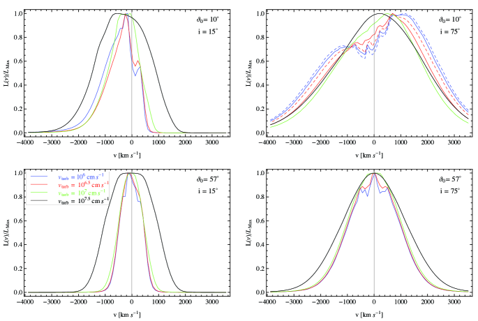
Figure 2: $L_{\nu}/L_{\mathrm{max}}$ versus velocity for 4 different values of the thermal plus turbulent velocity: $v_{\mathrm{turb}}=10^{6},10^{6.5},10^{7},10^{7.5}$ cm s^-1 and two different inclination angles: $i=15\degr$ (left panels) and $i=75\degr$ (right panels). Upper panels correspond to $\vartheta_{0}=10\degr$ and lower panels, to $\vartheta_{0}=57\degr$. The initial density is $n_{0}=10^{11}$ cm^-3 in all cases. The two extra curves shown in the upper right panel correspond to $v_{\mathrm{turb}}=10^{5.8}$ cm s^-1 (dashed blue) and $10^{6.2}$ cm s^-1 (dashed red).

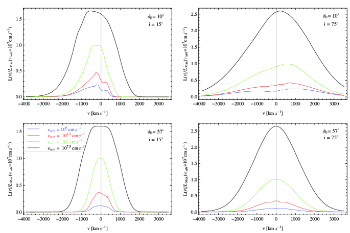
Figure 3: $L_{\nu}/L_{\mathrm{max}}(v_{\mathrm{turb}}=10^{7}$ cm s${}^{-1})$ versus velocity for four different values of the thermal plus turbulent velocity: $v_{\mathrm{turb}}=10^{6}$, $10^{6.5},10^{7},10^{7.5}$ cm s^-1 and two different inclination angles: $i=15\degr$ (left panels) and $i=75\degr$ (right panels). Upper panels correspond to $\vartheta_{0}=10\degr$ and lower panels, to $\vartheta_{0}=57\degr$.

These results suggested considering different velocities by incorporating the effect of turbulence. Bottorff & Ferland (2000) studied how microturbulence can affect the lines and showed that it affects more the far UV lines. Figure 2 shows the lines corresponding to four different values of $v_{\rm turb}$, for two different inclination angles, $i=15\degr$ (left panels) and $i=75\degr$ (right panels). The profiles in the upper row correspond to $\vartheta_{0}=10\degr$ and in the lower row, to $\vartheta_{0}=57\degr$. In general, the lines become smoother and more symmetric with increasing $v_{\rm turb}$. A much higher $v_{\mathrm{turb}}$ does make a noticeable difference, as expected. However, note that the upper right panel seems to represent an anomalous situation, as the profiles become narrower as the turbulent velocity increases.

To investigate the apparently anomalous situation in the upper right corner of Fig. 3 we plotted the same profiles as above, but normalized to the values corresponding to our fiducial turbulent velocity ($10^{7}$ cm s^-1). Note that in all cases, even in the apparently deviant case, the flux increases when the turbulent velocity does.

5.2 Changing inclination angle at fixed launching angle

For the fiducial values of density ($n_{0}=10^{11}$ cm^-3) and turbulent velocity ($v_{\rm turb}=10^{7}$ cm s^-1), we studied the effect(s) of changing the launching and viewing angles, in the ranges $\vartheta_{0}=5\degr-57\degr$ and $i=10\degr-84\degr$, respectively. The results are shown in Figures 4 and 5.

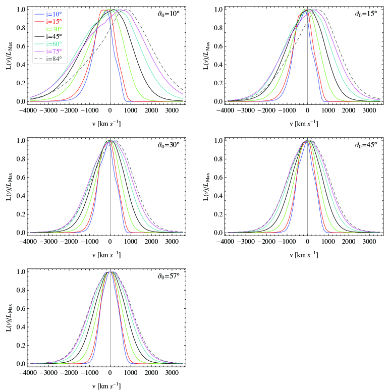
Figure 4: $L_{\nu}/L_{\mathrm{max}}$ versus velocity for $i=10\degr-84\degr$. Looking clockwise from the upper left: $\vartheta_{0}=10\degr,15\degr,30\degr,45\degr,57\degr$. The latter two cases do not differ significantly.

In each panel of Figure 4 the profiles are plotted versus velocity for a given launching angle, to enhance the effect of changing the viewing angle. Zero velocity is the average of the two doublet wavelengths. The velocities plotted represent velocities from the observer’s point of view, therefore negative velocities correspond to blueshifts. In all cases the profiles are slightly asymmetric, with increasing degree of asymmetry with decreasing inclination. The blue wings change less than the red wings, so that as the inclination angle approaches to smaller values, the red wings are increasingly weaker. In Figure 4, the effect is hard to notice for the lowest $\vartheta_{0}$ (the two upper panels), due to the shift to the red in the peak of the profiles when the inclination increases. We will discuss the effect of launching angle dependency below.

A way to see this is by noting that, for a given launching angle, when the object is seen face-on, the projection of the velocity into the line of sight is towards the observer for any azimuthal angle, while for objects seen edge-on, that projection is towards the observer for part of the emitting region, and receding from them for the rest. For intermediate cases, the closer the object’s LOS is to the face-on case, the more the red wing of its profile is weakened, explaining why the lines are less symmetric for smaller inclination angles.

5.3 Changing launching angle at fixed inclination angle

The effects of changing the launching angle $\vartheta_{0}$ are shown in Figure 5, where in each panel we have plotted the profiles for a given inclination angle and different launching angles. The actual angle to be considered is the angle $\vartheta$ at which a line launched with some $\vartheta_{0}$ crosses the base of the emitting region (when $\vartheta_{0}$ increases, so does $\vartheta$). For instance, for our chosen value of $\tan\beta$, for $\vartheta_{0}=20\degr$, $\vartheta\sim 25.82\degr$ and for $\vartheta_{0}=45\degr$, $\vartheta=48\degr$

When $\vartheta_{0}$ increases, the projection of the wind velocity onto the LOS is towards the observer in a portion of the emission region (i.e., for some azimuths) and is also towards the observer in the rest of the region as long as $\vartheta>i$. In the cases $\vartheta<i$, that projection is receding from the observer. As the wind velocity decreases with increasing $\vartheta_{0}$, so does the magnitude of its projection for given $i$, and thus the blueshift decreases for increasing $\vartheta_{0}$. However, it is the Doppler velocity, including a contribution from the rotational velocity, which is the velocity relevant for producing the observed line profiles. Thus, as the wind velocity decreases with $\vartheta$, then not only is the blueshift reduced, but the rotational velocity is increasingly dominant and the profiles become more symmetric. For any launch angle, the relative importance of the receding term with respect to the approaching term increases with increasing viewing angle, but the effect is larger for smaller $\vartheta_{0}$.

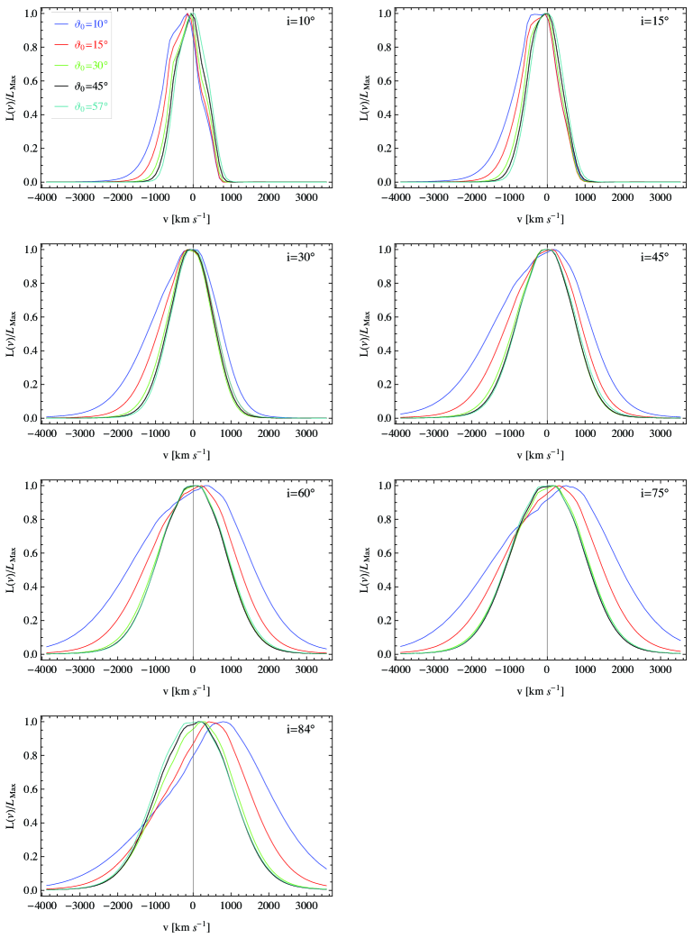
Figure 5: $L_{\nu}/L_{\mathrm{max}}$ versus velocity. In each panel, we have plotted the profiles corresponding to $i$ from $10\degr$ to $84\degr$ for $\vartheta_{0}=10\degr-57\degr$. For given $i$, those profiles for which $\vartheta>i$ are bluer, while those corresponding to $\vartheta<i$ are redder. Here, $\vartheta>\vartheta_{0}$ is the angle between a line launched with some $\vartheta_{0}$ and the base of the emitting region.

We also analysed how strongly this broadening of line profile with decreasing $\vartheta_{0}$ depends on the density profile. Note that, in principle, the smaller $\vartheta_{0}$ is, the larger the radii at which the streamlines intersect the base of the emission region, that is, these lines will form at radii where the density (that goes as $\sim r^{-b}$) is smaller, affecting the optical depth. To that end, we compared the inverse square power-law to other (less steep) density power-laws ($b=0.5,1$) for different launching angles, and found that the dependence is negligible. That is, the broadening found in the small $\vartheta_{0}$ cases depends mainly on the velocity projection.

In summary, the relevant quantity is neither of the angles, but a combination of them. This can also be seen by considering the expression of the optical depth (Eq. 11) where the frequency dependance is encompassed in the exponent $x_{\nu}$, dependent on the Doppler velocity $v_{\mathrm{D}}$. The latter includes the wind contribution, which ranges from $v_{\mathrm{p}}\sin(\vartheta+i)$ when $\phi=0$, to $v_{\mathrm{p}}\sin(\vartheta-i)$ when $\phi=\pi$. Note also, that the FWHM increases with increasing inclination angle (see Fig. 4), but for small launching angles it reaches its maximum at $i<84\degr$, while the maximum is reached at $i=84\degr$ for larger $\vartheta_{0}$. In the smaller $\vartheta_{0}$ cases, the broadening and subsequent decrement is accompanied by a shift in the peak, from bluer (at smaller inclinations) to redder velocities (at larger inclinations). This is due to the fact that the observer sees the base of the conical emission region from an almost edge-on perspective, so that the part of the cone with $\phi\simeq 0\degr$ (which produces blueshifted emission) has very small projected surface area.

5.4 Changing density

We also looked at the effects of varying the initial density. Although we adopted $n_{0}\sim 10^{11}$ cm^-3 as the “standard density”, we also chose to check the effect of even lower and higher densities. In principle, one would expect broader profiles for smaller initial density. In fact, that is what is found when running simulations that do not include the terms and factors introduced in Hall et al. (2012). In that case, the results showed that the profiles become broader as the initial density decreases. In effect, as the density decreases, so does the opacity and, in that case there will be less photons absorbed in the line wings and this translates into broader lines. However, the inclusion of these previously neglected terms and factors modifies the behaviour of the profiles, in such a way that the effect of changing the initial density is much less important (negligible, in some cases). In the current model, the velocity field (which depends on both inclination and launching angles) dictates the optical depth behaviour. This is somewhat similar to the broadening of the low-$\vartheta_{0}$ case that we discussed above.

Figure 6 shows the profiles obtained for a fixed inclination $i=15\degr$ (left panels) and $i=75\degr$ (right panels) and launching angles $\vartheta_{0}=15\degr$ (upper panels) and $\vartheta_{0}=57\degr$ (lower panels) when the initial density, which declines radially according to $n\sim r^{-2}$ is varied. The results of the density analysis also show that for given $\vartheta_{0}$, the smaller the inclination angle, the bluer the maximum. Note also that we have included two extra profiles in the upper right panel, to illustrate that in this particular case ($\vartheta_{0}=10\degr$, $i=75\degr$) the profiles do indeed converge at lower densities.

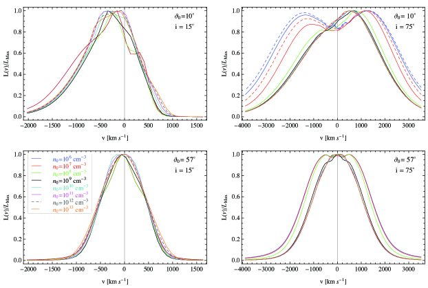
Figure 6: $L_{\nu}/L_{\mathrm{max}}$ versus velocity. Here, the profiles correspond to fixed $i\sim 15\degr$ (left panels) and $i\sim 75\degr$ (right panels) and $\vartheta_{0}=10\degr$ (upper panels) and $\vartheta_{0}=57\degr$ (bottom panels) but different initial densities: $n_{0}=10^{6}$ cm^-3 (blue), $n_{0}=10^{7}$ cm^-3 (red), $n_{0}=10^{8}$ cm^-3 (green), $n_{0}=10^{9}$ cm^-3 (black), $n_{0}=10^{10}$ cm^-3 (cyan), $n_{0}=10^{11}$ cm^-3 (magenta), $n_{0}=10^{12}$ cm^-3 (dashed gray) and $n_{0}=10^{13}$ cm^-3 (orange). The extra lines in the upper right panel correspond to $n_{0}=10^{5}$ cm^-3 (dashed blue) and $n_{0}=10^{6.5}$ cm^-3 (dashed red) and were included to show that, although slower than in other cases, the low-density profiles also converge. The effect of a lower density on the opacity, and thus on the line broadness, is surpassed by the effect of the velocity field, leaving a weak dependence on density, especially at lower inclinations. For fixed $\vartheta_{0}$ (i.e., looking along rows) the spread is larger for higher inclination angles, while for fixed $i$ (i.e, looking along columns), it is larger for smaller launching angle, with the trend being more pronounced with decreasing $n_{0}$.

5.5 Smaller launching angles

The effect of even smaller launching angles is shown in Figure 7 for the cases $i=5\degr,30\degr,75\degr$. Included, for comparison, are the profiles for the same inclination angles, but with $\vartheta_{0}=10\degr$. In the left panel, each profile is normalized with respect to the maximum of the $i=5\degr$ profile for each launching angle, whereas in the right panel the normalization is with respect to its own maximum. Two observations can be made from the figure. First, the differences between $\vartheta_{0}=5\degr$ and $\vartheta_{0}=10\degr$ profiles are much larger than those between $\vartheta_{0}=10\degr$ and $\vartheta_{0}=15\degr$ profiles. Second, when the viewing angle is large and $\vartheta_{0}=5\degr$, the profile is double-peaked, which is not observed in C iv  lines.

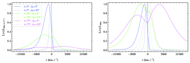
Figure 7: Two different normalizations of the profiles for $\vartheta_{0}=5\degr,10\degr$ and $i=5\degr,30\degr,75\degr$. In the left panel, the profiles are normalized to the maximum of the $i=5\degr$ for the corresponding launching angle. In the right panel, the normalization is with respect to each profile’s own maximum.

To study these issues we analysed the evolution of the profiles, for two different inclination angles ($i=5\degr,75\degr$), when the launching angle changes between $\vartheta_{0}=5\degr$ and $15\degr$. Figure 8 shows that in both cases, as the launching angle increases the profiles become increasingly narrower. Here we see the same trend shown in Figure 5 and discussed in subsection 5.3: for smaller launch and viewing angles (left panel), most of the flux is due to motion towards the observer and the blueshift decreases with increasing $\vartheta_{0}$. For larger $i$ (right panel) the contribution of the receding term of the Doppler velocity dominates but also decreases with increasing $\vartheta_{0}$, leading to an emission peak that approaches the systemic redshift with increasing $\vartheta_{0}$. Also noticeable is the fact that the double-peaked feature is only present when $\vartheta_{0}=5\degr$ (and to lower extent when $\vartheta_{0}=6\degr$). That suggests that we can impose an empirical restriction on $\vartheta_{0}$ and consider only those that satisfy the condition $\vartheta_{0}>6\degr$. To determine whether this is a general constraint, valid for any given $\beta$, would require simulations for different values of that parameter, which is beyond the scope of this work.

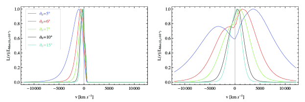
Figure 8: Normalized profiles for $\vartheta_{0}=5\degr$-$7\degr,10\degr,15\degr$ and $i=5\degr$ (left panel), $75\degr$ (right panel).

6 Line Width Measures

From a set of profiles obtained for different inclination angles $i$ and launching angles $\vartheta_{0}$ we study how the FWHMs are distributed as a function of the angles $i$ at which quasars are visible. To do so, we use an approach similar to that of Fine et al. (2008), who constrained the range of possible AGN viewing angles by using geometrical models for the BLR and comparing the expected dispersion in linewidths at each viewing angle to their observational data. We extend their analysis by also considering the clumpy torus model of Nenkova et al. (2008a, 2008b; hereafter N08), as constrained by Mor et al. (2009) using infrared observations of luminous AGN.

Fine et al. (2008) measured the linewidth of the Mg ii  line in 32214 quasar spectra from the Sloan Digital Sky Survey (SDSS) Data Release Five, 2dF QSO Redshift survey (2QZ) and 2dF SDSS LRG and QSO (2SLAQ) survey and found that the dispersion in linewidths strongly correlates with the optical luminosity of QSOs. Fine et al. (2010) used 13776 quasars from the same surveys to study the dispersion in the distribution of C iv  linewidths. In contrast to their findings for the Mg ii, they found that the dispersion in C iv  linewidths is essentially independent of both redshift and luminosity. Fine et al. (2008, 2010) used the fact that if the linewidth measured from a spectrum depends on the viewing angle to the object, the linewidth dispersion for a model for the BLR can by calculated by ‘observing’ that model over different ranges of viewing angles. Combinations of models and viewing angle ranges that give dispersions larger than the observed dispersion it can be rejected. Fine et al. assumed a coplanar obscuring torus surrounding the central SMBH and BLR with an opening angle $i_{\mathrm{max}}$ (measured from the vertical axis), so that the viewing angle $i$ should satisfy $i\leq i_{\mathrm{max}}$. If the FWHM of a BEL varies with $i$, the dispersion in the FWHM distribution of that BEL should vary with $i_{\mathrm{max}}$.

6.1 Fine et al. test

Following Fine et al. (2008), we compare the dispersion of observed $\log(\text{FWHM})$ values with the dispersion of our simulated $\log(\text{FWHM})$ as a function of $i_{\mathrm{max}}$ and launching angle $\vartheta_{0}$ to see if we can constrain $i_{\rm max}$ or $\vartheta_{0}$.

Using the launching angle as a parameter, we evaluate the dispersion of the function $f(i)=\log(\text{FWHM}(i))$. As all the variables are, in fact, continuous, we interpolated each set of FWHMs to obtain the corresponding continuous functions. For a given $i_{\mathrm{min}}$, the mean and the variance of the FWHMs are functions of $i_{\rm max}$, according to

$$\bar{f}(i_{\mathrm{max}})= \frac{\int_{i_{\mathrm{min}}}^{i_{\mathrm{max}}}\sin i\;P(i)\;f(i)\,di}{\int_{i_{\mathrm{min}}}^{i_{\mathrm{max}}}\sin i\;P(i)\,di}\,,$$ (53)

$$\sigma^{2}_{f}(i_{\mathrm{max}})= \frac{\int_{i_{\mathrm{min}}}^{i_{\mathrm{max}}}\sin i\;P(i)\;\left[f(i)-\bar{f}(i_{\mathrm{max}})\right]^{2}\,di}{\int_{i_{\mathrm{min}}}^{i_{\mathrm{max}}}\sin i\;P(i)\,di}\,,$$ (54)

where $P(i)$ is a weighting factor, equal to 1 in the Fine et al. (2008) approach, that measures the probability of not having obscuration in the LOS direction. We first present results using $P(i)=1$ and then turn to a more complex case. Both Fine et al. (2008) and Mor et al. (2009) have $i_{\mathrm{max}}=90\degr$ as the upper limit for that angle. However, we have an extra limitation, set by the inclination of the base of the emitting region, chosen to be $\beta=6\degr$. Therefore, our upper limit is $i_{\mathrm{max}}=84\degr$.

Noting that Fine et al. (2008, 2010) have employed inter-percentile values (IPVs) rather than FWHMs to characterize the line widths, we also investigated the behaviour of this line measure from our results. For a given percentage $p$, the definition of IPV$p$ suggested by Whittle (1985) is the separation between the median (where the integrated profile reaches the $50\%$ of the total flux) and the positions where $p\%$ and $(100-p)\%$ of the total flux are reached. Thus, calling $d_{1}$ and $d_{2}$ the distances between the median and $p$ and $(100-p)$ respectively, IPV$p=d_{1}+d_{2}$. Note that EBS92 define the analogous quantity $W_{x}$ (half-width at $x$), where $x$ is defined as a given fraction of the peak flux.

Figure 9 shows the averages (top panel) and dispersions (bottom panel) obtained for $\vartheta_{0}=5\degr,10\degr,15\degr,30\degr,45\degr,57\degr$ for different $i=i_{\mathrm{max}}$ ranging from $5\degr$ to $84\degr$ when $i_{\mathrm{min}}=2.5\degr$. Solid lines correspond to FWHM and dashed lines to IPV line width measurements. For most maximum inclination angles, for fixed $i_{\mathrm{max}}$, the dispersion of the FWHMs decreases with increasing $\vartheta_{0}$. In particular, the dispersion of FWHM for the smallest launching angle is systematically larger than for all others. We can see that the general trend is lower dispersion for higher $\vartheta_{0}$, except for the smaller $i_{\mathrm{max}}$, where $\sigma_{\vartheta_{0}=45\degr}$ departs from it.

We also compared these results to a simple model which assumes $g(i)=\text{FWHM}(i)=i(\,1000$ km s^-1), merely to see how the dispersion in log(FWHM) behaves for a model with known variation of FWHM with $i$. The dotted line in Figure 9 corresponds to this simple model. For the $i_{\mathrm{min}}$ considered in the figure, this model departs from the observational results at any $\vartheta_{0}$. We found that when $i_{\rm min}=7.5\degr$, the model approximately matches the result for $\vartheta_{0}=5\degr$ in the range $35\degr\lesssim i_{\mathrm{max}}\lesssim 60\degr$. In the general case, it can be inferred that a more sophisticated model is needed. Such a model probably has to include information about the launching angle.

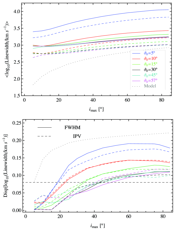
Figure 9: Averages (top panesl) and dispersions (bottom panel) of $\log(\text{FWHM})$ (solid lines) and $\log(\text{IPV25})$ (dashed lines) evaluated for different launching angles, using $P(i)=1$. The minimum viewing angle is $i_{\mathrm{min}}=2.5^{\circ}$. Included is the plot (dotted curve) of the dispersion for a model of the form $g(i)=\text{FWHM}(i)=i(1000\text{ km s}^{-1})$ (see text). The dashed horizontal line plotted together with the dispersions corresponds to the Fine et al. (2010) results, its meaning is commented below.

The dispersions obtained for the FWHMs are increasing functions of the parameter $i_{\mathrm{max}}$, although they show a mild decreasing trend at $i_{\mathrm{max}}\gtrsim 60\degr$. Similarly, the dispersions of the IPVs are increasing functions of $i_{\rm max}$. Also included in Figure 9 is the 0.08 dex dispersion line reported by Fine et al. (2010) as the observational upper limit on the dispersion measured from their sample. We can see that as the torus half-opening angle (measured from the polar axis, and represented by $i_{\mathrm{max}}$) increases above about $18\degr$, the wind launch angles required to match the Fine et al. (2010) constraints are increasingly larger.

Figure 10 shows the allowed region in the $i$-$\vartheta_{0}$ plane when analysing the dispersion of FWHMs (left panel) and of IPV25s (right panel). In both cases, $i_{\mathrm{min}}=2.5\degr$. Our results give, within the $\vartheta_{0}<60\degr$ range allowed by the MHD solutions, a maximum half-opening angle of about $47\degr$, above which no wind launch angle matches the observations. This maximum torus half-opening angle has a somewhat different behaviour if the IPVs are considered, reaching a maximum at $\vartheta_{0}\sim 30\degr$ and declining for larger $\vartheta_{0}$. However, note that the “absolute” maximum is similar in both cases.

Figure 10: Contour plot of the standard deviation of the FWHM vs launching and inclination angles. Only the contours within the region that matches the Fine et al. results are shown.

In section 5 we showed that the profiles obtained for cases corresponding to larger inclination and small launching angle had double-horned profiles and mentioned that this contradicts observational results. The analysis presented in this section shows that such combinations are in fact ruled out.

6.2 Clumpy torus

As mentioned above, Mor et al. (2009) adopted the more detailed expression for the escape probability proposed by N08. In that model, the torus is clumpy, consisting of optically thick clouds and the quasar is obscured when one of such clouds is seen along the LOS. The torus is characterized by the inner radius of the cloud distribution (set to the dust sublimation radius, $R_{\mathrm{d}}$, that depends on the grain properties and mixture) and six other parameters. Equation (3) in Mor et al. (2009) provides the weighting factor that we used in our evaluation:

$$P_{\mathrm{esc}}(i)=\exp\left[{-N_{0}\exp\left({-\frac{(\pi/2-i)^{2}}{\sigma^{2}}}\right)}\right]$$ (55)

where $N_{0}$ is the mean number of clouds along a radial equatorial line and $\sigma$ is the torus width parameter (analogous to its opening angle). Implicitly, it is assumed that the disc and the torus are aligned. In their Fig. 6, Mor et al. (2009) present the torus parameter distributions for their sample, and from there it is clear that the distribution of the two parameters we need to input in Eq. 55 (namely, $N_{0}$ and $\sigma$) are very broad. For completeness, we have reproduced in Table 2 the minimum, mean and maximum values of the two parameters, taken from Mor et al. (2009). Note that within this model, we only have $i_{\mathrm{max}}=\pi/2$. The resulting distribution of the dispersions with the launching angle are presented in Figure 11, where each line corresponds to a given combination of $\sigma$ and $N_{0}$. For clarity, in the figure we excluded combinations such that at least one of the parameters takes its minimum value, as such combinations yield lines farther away from the observed upper limit dispersion.

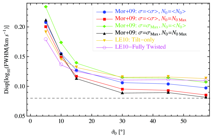
Figure 11: Dispersions of $\log(\text{FWHM})$ using $P(i=\pi/2-\beta)$ as given by Eq. 55. Here, $i_{\mathrm{min}}=2.5\degr$, $i_{\mathrm{max}}=84\degr$. Each of the lines obtained using the Mor et al. (2009) prescription represents a different combination of $\sigma$ and $N_{0}$. Also included is a line corresponding to dispersions calculated assuming a tilt-only warped disc (see next section). The dashed line corresponds to the Fine et al. (2010) results.

Table 2: Minimum, mean and maximum values of the $N_{0}$ and $\sigma$ torus parameters from the Mor et al. (2009) sample.

Parameter	Minimum	Mean	Maximum
$N_{0}$	1	4.923	8
$\sigma$ [$\degr$]	15	34	57

For $\vartheta_{0}\lesssim 30\degr$, all cases depart significantly from the Fine at al. result. For $\vartheta_{0}\gtrsim 30\degr$, most cases remain highly incompatible with the Fine et al. results, but the curves are closer to them when $N_{0}=\max(N_{0}^{\mathrm{Mor+09}})$, with $\sigma=\max(\sigma^{\mathrm{Mor+09}})$ and $\sigma=\bar{\sigma}^{\mathrm{Mor+09}}$. That motivated us to look for combinations of these parameters such that the results based on Mor et al. (2009) model match the Fine et al. limit, at least for some launch angles. Adopting $\sigma=\bar{\sigma}^{\mathrm{Mor+09}}$ and increasing $N_{0}$, one finds that for $N_{0}\sim 15$ (the likely uppr limit, according to N08), all dispersions corresponding to $\vartheta_{0}\gtrsim 30\degr$ are below the Fine et al. boundary and the rest have decreased in a similar amount (the effect is that the curve has almost rigidly moved down). When $N_{0}\sim 30$, only dispersions corresponding to $\vartheta_{0}\lesssim 15\degr$ are above the Fine et al. boundary. If, instead, $\sigma=\max(\sigma^{\rm Mor+09})$ is adopted, for $N_{0}\sim 8.5$ the dispersion corresponding to $\vartheta_{0}\sim 57\degr$ is already below the Fine et al. limit, and for $N_{0}\sim 13.5$, all dispersions for the cases $\vartheta_{0}\gtrsim 15\degr$ are below that line. On the other hand, keeping $N_{0}=\max(N_{0}^{\rm Mor+09})$ and increasing $\sigma$ does not lead to an improvement.

Note that Mor et al. (2009) found $P(i=50\degr)\simeq 30\%$ and $P(i=70\degr)<3\%$ when $N_{0}$ and $\sigma$ were set to their mean values, and, based on that, suggested that the inclination angle for type-1 objects should lie in the range $0\degr-60\degr$. However, the authors found that for the case in which all the parameters but the torus width are set to their mean values, the escape probability falls rapidly if $\sigma>45\degr$. Our results indicate that the parameter $N_{0}$ is important when considering the dispersions of the line widths. In effect, as mentioned above, the only curves that are relatively close to the Fine et al. (2010) constraints correspond to the case $N_{0}=\max{(N_{0}^{\rm Mor+09})}$ and to have a better match larger $N_{0}$ values are needed. In that case, the $\sigma$ values should still be close to or larger than the mean from the Mor et al. (2009) sample.

These results were obtained from a set of profiles corresponding to both mass and luminosity fixed, whereas Fine et al. (2010) and Mor et al. (2009) samples involve a range of masses and luminosities. However, as already mentioned, Fine et al. (2010) found that the dispersion in C iv  linewidths essentially does not depend on luminosity. As can be seen from their Figure 2, the IPV linewidth measurements are bound by $10^{8.25}\lesssim M_{\mathrm{BH}}/M_{\sun}\lesssim 10^{10}$ and $0.1\lesssim L/L_{\mathrm{Edd}}\lesssim 1$. Based ion that, we then anticipate that our results would not be strongly affected by considering different masses and/or luminosities.

7 Warped Discs

As mentioned in the Introduction, the model of Lawrence & Elvis (2010, LE10 hereafter) replaces the torus by a warped disc. In this section we explore whether we can infer new constraints on the BLR or on the parameters of warped discs by applying a restricted set of such warped disc models. Briefly, we evaluate the unobscured solid angle distribution as a function of observer inclination $i$, $dC(i)$, calculated for arbitrary disc tilt angle $\theta$. Then, we restrict our attention to the subset within our constraint $i<\pi/2-\beta$, using the calculated unobscured solid angle distribution to determine the probability of the object being unobscured. Finally, we apply that probability to our emission line profiles, in a way analogous to that employed with the Fine et al. (2010) model.

LE10 studied the fraction of type 2 AGN, $f_{2}\approx 0.58$ among all AGN, and proposed a framework to account for it. They assumed that randomly directed infalling material at large scales would produce a warped disc at smaller scales, where it eventually aligns with the inner disc. They analysed both fully twisted and tilt-only cases (explained in detail below) under that assumption and showed that fully twisted discs can not reproduce the observed $f_{2}$. Models assuming tilt-only discs, on the other hand, match the observed $f_{2}$.

A warped disc can be analysed as a series of annuli, each characterized by its radius and the two angles $\theta(r)$ (the angle between the spin axes of the annulus and the inner planar disc, i.e., the tilt) and $\phi(r)$ (the angle of the line of nodes measured with respect to a fixed axis on the equatorial plane, i.e., the twist). Thus, a fully twisted disc corresponds to $\phi(r)=0$, $\phi(r+\delta r)=2\pi$, $\delta r\ll r$ and a tilt-only disc corresponds to the case of constant $\phi(r)$. Each of the two warp modes can be associated to a covering factor $C$ depending on the misalignment, and the distribution of covering factors can then be inferred from the probability distribution of the misalignment. Conversely, knowing the distribution of covering factors, the probability distribution of misalignments can be evaluated. This is the approach we take below. Note that LE10 calculated the azimuthally integrated covering factor while we study the covering fraction as a function of the azimuth.

Consider first the tilt-only case. In Appendix A we derive the expression for the differential covering factor $dC(i)$ corresponding to this case. We estimated the unobscured fraction $P(i)=dC(i)/2\pi\sin(i)$ as a function of the tilt angle and found that considering a random distribution in solid angle of $\theta$ up to $\theta_{\mathrm{max}}=\pi$ yields results incompatible with our line profiles. This is because that case corresponds to $i_{\rm max}=\pi/2$ for the Fine et al. case in all our diagrams. In a random distribution of incoming orientations with $\theta_{\mathrm{max}}=\pi$, for every case of orientation $\theta$ there is a corresponding case with orientation $\pi-\theta$ (statistically speaking), which means that this model is identical to the case $i_{m}ax=pi/2$ for our purposes. A variant of that model, with a random distribution in solid angle of $\theta$ up to $\theta_{\mathrm{max}}=\pi/2$ was also analysed. Using equation 62 for the probability and equations 53 and 54 we performed the same analysis applied in the Fine at al. case. Note that the only angle to be considered in this case is $i_{\rm max}=\pi/2$, so we also ruled out this model. We have included in Figure 11 the resulting dispersions for this model. The dispersions are far from the Fine et al. (2010) observational results for any launch angle considered.

An analogous analysis was performed for the full twist case, with $0\leqslant\theta\leqslant\pi/2$. The probability of being unobscured for random inclinations is given by $P(i)=\cos(i)$ and, again, the region in the $i-\vartheta_{0}$ plane is the same obtained using other prescriptions.

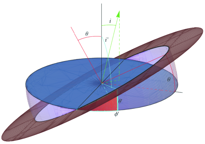
Figure 12: Representation of a tilt-only disc (warped but not twisted). The outermost disc (shown here as an annulus) is tilted at an angle $\theta$ with respect to the inner disc. That is also the angle between the spin axes of the annulus and the inner disc. The transition from outer disc to inner disc occurs over a range of radii in reality, but is shown here happening at a single radius for convenience. Adopting the azimuth of the ascending node as $\phi=0$, at azimuth $\phi^{\prime}$ the obscuration from the outer disc extends an angle $\theta^{\prime}$ above the inner disc given by $\sin(\theta^{\prime})=\sin(\theta)\sin(\phi^{\prime})$. The equivalent polar angle $i^{\prime}=\frac{\pi}{2}-\theta^{\prime}$ is given by $\cos(i^{\prime})=\sin(\theta)\sin(\phi)$. At each azimuth, the light purple shading represents the obscuration due to the tilted disc (which takes the form of two wedges, each of maximum width $\theta$). The light shadow represents the obscuration due to the tilted disc at all azimuths. The region at azimuths $0\leq\phi\leq\phi^{\prime}$ has a darker shadow to emphasize the angles intervening in the $\theta^{\prime}$ calculation.

8 Summary and Conclusions

In this paper, we combined an improved version of the MC97 disc wind model (Hall et al. 2012, in preparation) with the MHD driving of EBS92. We analysed how the resulting line profiles depend on different parameters of the model. In particular, we studied how the observing angle $i$ and the wind launch angle $\vartheta_{0}$ affect the emission line profiles. We found that for fixed $\vartheta_{0}$ all profiles are slightly asymmetric, with more asymmetric profiles for smaller inclination. For a given launching angle, less inclined objects have a larger fraction of their flux corresponding to motion towards the observer, therefore their profiles are less symmetric. For fixed $i$, the angle to be considered is $\vartheta>\vartheta_{0}$ , i.e the angle at which a wind that started at $\vartheta_{0}$ intercepts the base of the emitting region. Two different cases can be found. If $\vartheta>i$, wind velocity projections are mostly towards the observer, with red wings increasingly important for the cases $\vartheta\leq i$.

Our main conclusion is that the shape of the line profiles, their FWHMs and shift amounts (whether red or blue) with respect to the systemic velocity depend not only on the viewing angle but also on the angle (with respect to disc plane) at which the outflow starts. In fact, the relevant quantity is neither of the angles, but a combination of them. This is a consequence of how the model has been constructed. In effect, the optical depth expression includes a dependance on the wind contribution, which ranges from $v_{\mathrm{p}}\sin(\vartheta+i)$ when $\phi=0$, to $v_{\mathrm{p}}\sin(\vartheta-i)$ when $\phi=\pi$. The launch angle parameter, although included in the models, has been less explored in the literature. Note, however, that MC97 have reported that their C iv  line profiles do not strongly depend on $\vartheta_{0}$ ($\lambda_{0}$ in their notation). This difference could be due to our use of EBS92 streamlines instead of MC97 streamlines, or it could be due to our more rigorous calculation of $L_{\nu}$ as compared to MC97. Similar results opposite to our findings are reported by (Flohic et al.2012), in their study of Balmer emission lines.

Using as a constraint the observational results obtained by Fine et al. (2010) for the C iv  lines in their sample, we found that the allowed region in the $i-\vartheta_{0}$ plane has an upper limit that depends on the torus half-opening angle, $i_{\mathrm{max}}$. For instance, a launch angle $\vartheta_{0}\sim 7\degr$ is only allowed for torus half-opening angle $\lesssim 20\degr$, while $\vartheta_{0}$ is $\lesssim 25\degr$ for $i_{\rm max}\sim 40\degr$. We found that the maximum torus half-opening torus angle that is compatible with the observations is about $47\degr$. Considering a model that replaces the torus with a tilt-only warped disc, formed by the alignment at smaller distances of material falling at large distances from random directions, yields no difference in the resulting allowed region of the inclination-launch angle plane.

These results were obtained for a single mass and luminosity, as opposed to the Fine et al. (2010) and Mor et al. (2009) results which were obtained from datasets spanning an order of magnitude in both parameters. However, as mentioned in section 6, Figure 2 of Fine et al. (2010) indicates a mild dependence of the dispersion of the linewidth on both these parameters. Thus, we expect that simulations for different masses and luminosities (currently being undertaken) will yield similar results to those reported here. Future work will also consider applying the model to other high ionization lines, such as Si iv, as well as low ionization lines, such as Mg ii.

Other properties of the observed line profiles that could be measured and compared against the model include the line asymmetry (e.g. Whittle, 1985, EBS92) and the cuspiness at $x$, $C_{x}$, related to the kurtosis and proposed by EBS92, where $x$ is defined as a given fraction of the peak flux. In their analysis of Balmer lines, (Flohic et al.2012) have also studied other line profile moments. In addition to the FWHM, they considered the full width at quarter maximum (FWQM) as well as the asymmetry and kurtosis indexes (A.I. and K.I. respectively), and centroid shift at quarter maximum ($v_{\mathrm{c}}(1/4)$) as defined by Marziani et al. (1996). The present work does not include the treatment of resonance scattering of continuum photons or general relativistic (GR) effects. In their improvement of the MC97 and Chiang & Murray (1996) models, (Flohic et al.2012) found that when relativistic effects are included, the line profiles become skewed to the red. For a given combination of parameters, the line wings and centroids are increasingly redshifted with decreasing inclination. The amount of redshift is also a decreasing function of the inner radius of the line-emitting region, that satisfies $r_{\mathrm{min}}\geq 100\,r_{\mathrm{g}}$, where $r_{\mathrm{g}}$ is the gravitational radius. Although their results correspond to Balmer (i.e., low ionization) lines, we expect that high ionization lines such as C iv  may exhibit a similar or stronger response if the GR effects were to be considered, as C iv  is expected to be emitted predominantly at smaller radii. However, our analysis and that of (Flohic et al.2012) utilize different velocity fields, and therefore a comparison of our results and theirs is perhaps not straightforward. Giustini & Proga (2003) treat the absorption line dependence on wind geometry but we have not found in the literature a similar study for emission lines. The relativistic MHD case has been studied by several authors, often in the context of jet launching and collimation and in relation to several different astrophysical environments, such as AGN, microquasars, young stellar objects, pulsars and gamma-ray burst. The problem has been considered both in the steady (e.g. Camenzind, 1986; Chiueh et al., 1991; Li et al., 1992; Contopoulos, 1994, 1995; Fendt & Greiner, 2001; Heyvaerts & Norman, 2003) and in the time-dependent regimes (e.g. Koide et al., 1999; Porth & Fendt, 2010). In the relativistic MHD framework, the line formation problem has been considered in the X-ray range in relation to the iron K-line (e.g. Müller & Camenzind04, 2004). However, to the knowledge of the authors, the combination with a relativistic version of MC97 has not been yet explored in the literature. We consider that as one of the possible future lines of work to pursue.

Appendix A Unobscured Sightline Distribution for Tilt-only Discs

Below we outline the evaluation of $dC(i)$ for arbitrary disc tilt angle $\theta$, to within the numerical factor required so that the total probability in a given situation is unity. Recall that in the following analysis the covering fraction is a function of the azimuth, while it is azimuthally integrated in the calculations of LE10.

Define the line of nodes of the tilted outer disc relative to the inner disc to be at $\phi=0$. Then at each $\phi$, the obscuration from the outer disc extends an angle $\theta^{\prime}$ above the inner disc given by $\sin\theta^{\prime}=\sin(\theta)\sin(\phi)$ above the inner disc (sine rule for spherical right triangles); see Figure 12.

The equivalent polar angle $i^{\prime}=\frac{\pi}{2}-\theta^{\prime}$ is given by $\cos(i^{\prime})=\sin(\theta)\sin(\phi)$. Solving the latter equation for the maximum unobscured $\phi$ at a given $i$, $\phi_{\mathrm{max}}(i,\theta)$, yields

$$\phi_{\mathrm{max}}(i,\theta)=\arcsin[\cos(i)/\sin\theta],$$ (56)

where $0<\phi_{\mathrm{max}}(i,\theta)<\frac{\pi}{2}$.

For $0<\theta<\frac{\pi}{2}$, there is an unobscured polar cap (at $i<\frac{\pi}{2}-\theta$) and a region where obscuration increases from 0% at $i=\frac{\pi}{2}-\theta$ to 50% at $i=\frac{\pi}{2}$. The differential solid angle in each region is:

$$dC\left(i<\frac{\pi}{2}-\theta\right) =2\pi\sin(i)di$$ (57)

$$dC\left(\frac{\pi}{2}-\theta<i<\frac{\pi}{2}\right) =\sin(i)di\left(\pi+2\int_{\phi=0}^{\phi_{\mathrm{max}}(i,\theta)}d\phi\right)$$

$$=\sin(i)di\left(\pi+2\arcsin\left[{\cos(i)\over\sin\theta}\right]\right)$$ (58)

For $\frac{\pi}{2}<\theta<\pi$, there is a polar cap of complete obscuration $(i<\theta-\frac{\pi}{2})$ and a region where obscuration decreases from 100% at $i=\theta-\frac{\pi}{2}$ to 50% at $i=\frac{\pi}{2}$. The differential solid angle in the partially unobscured region is:

$$\begin{split}dC\left(\frac{\pi}{2}+\theta<i<\pi\right)&=\sin(i)di\left(\pi-2\int_{\phi=0}^{\phi_{\mathrm{max}}(i,\theta)}d\phi\right)\\ &=\sin(i)di\left(\pi-2\arcsin\left[{\cos(i)\over\sin\theta}\right]\right)\end{split}$$ (59)

For $0<\theta<\frac{\pi}{2}$, large $i$ values are underrepresented, while small $i$ values are underrepresented for $\frac{\pi}{2}<\theta<\pi$. At $\theta=\frac{\pi}{2}$, the half of the hemisphere with $0<\phi<\pi$ is obscured, which leads to a uniform 50% reduction in the probability of observing the quasar along every sightline as compared to the no-obscuration case.

A.1 Random orientations with $0\leq\theta\leq\frac{\pi}{2}$.

Here we analyse in more detail a restricted variant of the model where instead of a fixed tilt angle $\theta$, a distribution of such angles randomly distributed in solid angle from $0\leq\theta\leq\frac{\pi}{2}$ is considered. Combining equations 57 and 58 we obtain:

$$\begin{split}dC(i)&=\sin(i)di\Biggl{[}\int_{\theta=0}^{\frac{\pi}{2}-i}2\pi\sin\theta d\theta\,+\\ &\int_{\theta=\frac{\pi}{2}-i}^{\frac{\pi}{2}}\left(\pi+2\arcsin\left[{\cos(i)\over\sin\theta}\right]\right)\sin\theta d\theta\Biggr{]},\end{split}$$ (60)

which becomes

$$\begin{split}dC(i)&=\sin(i)di\Biggl{[}2\pi-\pi\cos\left(\frac{\pi}{2}-i\right)\\ &+2\int_{\theta=\frac{\pi}{2}-i}^{\frac{\pi}{2}}\arcsin\left[{\cos(i)\over\sin\theta}\right]\sin\theta d\theta\Biggr{]}\end{split}$$ (61)

From $dC(i)$ we define $P(i)$, the probability of being unobscured, as

$$P(i)=\frac{dC(i)}{2\pi\sin(i)}.$$ (62)

In the text, we comment on the results of combining the latter expression with equations 53 and 54 to perform the same analysis applied in the Fine at al. case.

References

- Arav et al. (1998) Arav et al., 1998, MNRAS, 297, 990
- Baldwin et al. (2003) Baldwin J. A. et al., 2003, ApJ, 582, 590
- Batchelor (1967) Batchelor, G.K., 1967, An Introduction to Fluid Mechanics, Cambridge University Press, Appendix 2
- Blandford & Payne (1982) Blandford, R. D., Payne, D. G., 1982, MNRAS, 1999, 883
- Bottorff et al. (1997) Bottorff M. C., Korista K. T., Shlosman I., Blandford R. D., 1997, ApJ, 479, 200
- Bottorff & Ferland (2000) Bottorff M. C., Ferland G. J., 2000, MNRAS, 316, 103
- Camenzind (1986) Camenzind, M., 1986, A&A, 156, 137
- Chiang & Murray (1996) Chiang J., Murray N., 1996, ApJ, 466, 704
- Chiueh et al. (1991) Chiueh, T., Li, Z.-Y., & Begelman, M. C., 1991, ApJ, 377, 462
- Contopoulos & Lovelace (1994) Contopoulos J., Lovelace R.V.E., 1994, ApJ. 429, 139
- Contopoulos (1994) Contopoulos, J. 1994, ApJ, 432, 508
- Contopoulos (1995) Contopoulos, J. 1995, ApJ, 446, 67
- Dietrich et al. (1999) Dietrich M., Wagner S. J., Courvoisier T. J. L., Bock H., North P., 1999, A&A, 351, 31
- Elitzur (2008) Elitzur M., 2008, NewAR, 52, 274
- Emmering et al. (1992) Emmering R. T., Blandford R. D., Shlosman I., 1992, ApJ, 385, 460
- Everett (2005) Everett J., 2005, ApJ, 631, 689
- Fendt & Greiner (2001) Fendt C., Greiner J., 2001, A&A 369, 308
- Ferreira & Pelletier (1995) Ferreira J., Pelletier G., 1995, A&A 295, 807
- Fine et al. (2008) Fine S., et al., 2008, MNRAS, 390, 1413
- Fine et al. (2010) Fine S. et al., 2010, MNRAS, 409, 591
- (21) Flohic H. M. L. G., Eracleous M., Bogdanović T., 2012, ApJ, 753, 133
- Giustini & Proga (2003) Giustini M., Proga D., 2012, ApJ, 758, 70
- Groves (2007) Groves, B., 2007, in Ho L. C., Wang J. W., eds, ASP Conf. Ser. 373, The Central Engine of Active Galactic Nuclei, ASP, San Francisco, p. 511
- Heyvaerts (1996) Heyvaerts, J., 1996, in Chiuderi C., Einaudi, Giorgio, eds, Plasma Astrophysics, Springer-Verlag, Berlin, p. 31
- Heyvaerts & Norman (2003) Heyvaerts J., Norman C., 2003, ApJ, 596, 1240
- Kaspi & Netzer (1999) Kaspi S., Netzer H., 1999, ApJ, 524, 71
- Kaspi et al. (2007) Kaspi S. et al., 2007, ApJ, 659, 997
- Koide et al. (1999) Koide S., Shibata K., Kudoh T., 1999, ApJ, 522, 727
- Königl (1989) Königl A., 1989, ApJ, 342, 208
- Königl & Kartje (1994) Königl A., Kartje J. F. 1994, ApJ, 434, 446
- Korista (1999) Korista K., 1999, in Ferland G., Baldwin J., eds, ASP Conf. Ser. 162, Quasars and Cosmology, ASP, San Francisco, p. 165
- Lawrence & Elvis (2010) Lawrence A., Elvis M., 2010, ApJ, 714, 561
- Li et al. (1992) Li Z., Chiueh T., Begelman M. C., 1992, ApJ, 394, 459
- Mathews & Capriotti (1985) Mathews W. G., Capriotti E. R., 1985, in Miller J. S., ed., Astrophysics of Active Galaxies and Quasi-Stellar Objects. Univ. Science Books, Mill Valley, CA, p. 185
- Mestel (1968) Mestel L., 1968, MNRAS, 138, 359
- Mor et al. (2009) Mor R., Netzer H., Elitzur M., 2009, ApJ, 705, 298
- Müller & Camenzind04 (2004) Müller A., Camenzind M., 2004, A&A, 413, 861
- Murray et al. (1995) Murray N. et al., 1995, ApJ, 451, 498
- Murray & Chiang (1997) Murray N., Chiang J., 1997, ApJ, 474, 91
- Murray & Chiang (1998) Murray N., Chiang J. 1998, ApJ, 494, 125
- Nenkova et al. (2008) Nenkova M. et al., 2008, ApJ, 685, 147
- Nenkova et al. (2008) Nenkova M. et al., 2008, ApJ, 685, 160
- Netzer (1990) Netzer H., 1990, in Blandford R. D., Netzer H., Woltjer L., eds, Saas-Fee Advanced Course 20: Active Galactic Nuclei Springer-Verlag, Berlin, p. 57
- Porth & Fendt (2010) Porth O., Fendt C., 2010, IJMPD,19, 677
- Rybicki & Hummer (1978) Rybicki G. B., Hummer D. G., 1978, ApJ, 219, 654
- Rybicki & Hummer (1983) Rybicki G. B., Hummer D. G., 1983, ApJ, 274, 380
- Sulentic et al. (1995) Sulentic J. W. et al., 1995, ApJ, 445, 85
- Sulentic et al. (2000) Sulentic J. W., Marziani P., Dultzin-Hacyan, D., 2000, ARA&A, 38, 521
- Vanden Berk et al. (2001) Vanden Berk D. E. et al., 2001, AJ, 122, 549
- Whittle (1985) Whittle, M., 1985, MNRAS, 213, 1