Inferring the Origin Locations of Tweets
with Quantitative Confidence

Abstract

Social Internet content plays an increasingly critical role in many domains, including public health, disaster management, and politics. However, its utility is limited by missing geographic information; for example, fewer than 1.6% of Twitter messages (tweets) contain a geotag. We propose a scalable, content-based approach to estimate the location of tweets using a novel yet simple variant of gaussian mixture models. Further, because real-world applications depend on quantified uncertainty for such estimates, we propose novel metrics of accuracy, precision, and calibration, and we evaluate our approach accordingly. Experiments on 13 million global, comprehensively multi-lingual tweets show that our approach yields reliable, well-calibrated results competitive with previous computationally intensive methods. We also show that a relatively small number of training data are required for good estimates (roughly 30,000 tweets) and models are quite time-invariant (effective on tweets many weeks newer than the training set). Finally, we show that toponyms and languages with small geographic footprint provide the most useful location signals.

1 Introduction

Applications in public health [9], politics [29], disaster management [21], and other domains are increasingly turning to social Internet data to inform policy and intervention strategies. However, the value of these data is limited because the geographic origin of content is frequently unknown. Thus, there is growing interest in the task of location inference: given an item, estimate its geographic true origin.

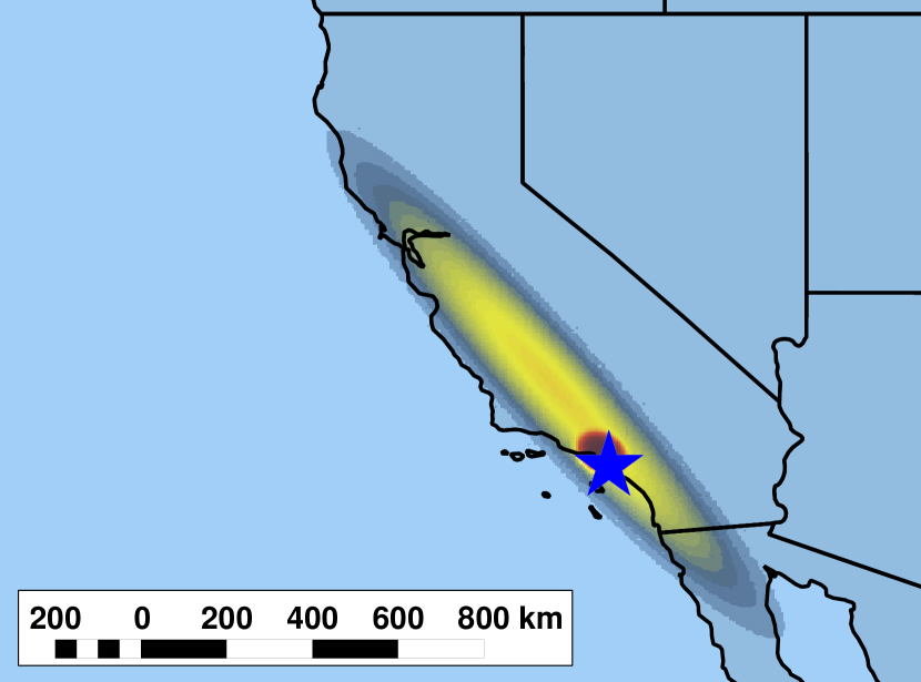
text:	Americans are optimistic about the economy & like what Obama is doing. What is he doing? Campaigning and playing golf? Ignorance is bliss
language:	en
location:	Los Angeles, CA
time zone:	pacifictimeuscanada

Figure 1: A tweet originating near Los Angeles, CA. We show the true origin (a blue star) and a heat map illustrating the density function that makes up our method’s estimate. This estimate, whose accuracy was at the 80th percentile, was driven by two main factors. The unigram ca from the location field, visible as the large density oval along the California coast, contributed about 12% of the estimate, while angeles ca, the much denser region around Los Angeles, contributed 87%. The contribution of four other n-grams (angeles, los angeles, obama, and los) was negligible.

We propose an inference method based on gaussian mixture models (GMMs) [22]. Our models are trained on geotagged tweets, i.e., messages with user profile and geographic true origin points. For each unique n-gram, we fit a two-dimensional GMM to model its geographic distribution. To infer the origin of a new tweet, we combine previously trained GMMs for the n-grams it contains, using weights inferred from data; Figure 1 shows an example estimate. This approach is simple, scalable, and competitive with more complex approaches.

Location estimates using any method contain uncertainty, and it is important for downstream applications to quantify this uncertainty. While previous work considers only point estimates, we argue that a more useful form consists of a density estimate (of a probability distribution) covering the entire globe, and that estimates should be assessed on three independent dimensions of accuracy, precision, and calibration. We propose new metrics for doing so.

To validate our approach, we performed experiments on twelve months of tweets from across the globe, in the context of answering four research questions:

1. Improved approach. How can the origin locations of social Internet messages be estimated accurately, precisely, and with quantitative uncertainty? Our novel, simple, and scalable GMM-based approach produces well-calibrated estimates with a global mean accuracy error of roughly 1,800 km and precision of 900,000 square kilometers (or better); this is competitive with more complex approaches on the metrics available in prior work.

2. Training size. How many training data are required? We find that approximately 30,000 tweets (i.e., roughly 0.01% of total daily Twitter activity) are sufficient for high-quality models, and that performance can be further improved with more training data at a cost of increased time and memory. We also find that models are improved by including rare n-grams, even those occurring just 3 times.

3. Time dependence. What is the effect of a temporal gap between training and testing data? We find that our models are nearly independent of time, performing just 6% worse with a gap of 4 months (vs. no gap).

4. Location signal sources. Which types of content provide the most valuable location signals? Our results suggest that the user location string and time zone fields provide the strongest signals, tweet text and user language are weaker but important to offer an estimate for all test tweets, and user description has essentially no location value. Our results also suggest that mentioning toponyms (i.e., names of places), especially at the city scale, provides a strong signal, as does using languages with a small geographic footprint.

The remainder of our paper is organized as follows. We first survey related work, then propose desirable properties of a location inference method and metrics which measure those properties. We then describe our experimental framework and detail our mixture model approach. Finally, we discuss our experimental results and their implications. Appendices with implementation details follow the body of the paper.

2 Related Work

Over the past few years, the problem of inferring the origin locations of social Internet content has become an increasingly active research area. Below, we summarize the four primary lines of work and contrast them with this paper.

2.1 Geocoding

Perhaps the simplest approach to location inference is geocoding: looking up the user profile’s free-text location field in a gazetteer (list of toponyms), and if a match is found, inferring that the message originated from the matching place. Researchers have used commercial geocoding services such as Yahoo! Geocoder [32], U.S. Geological Survey data [26], and Wikipedia [16] to do this. This technique can be extended to the message text itself by first using a geoparser named-entity recognizer to extract toponyms [13].

Schulz et al. [30] recently reported accurate results using a scheme which combines multiple geocoding sources, including Internet queries. Crucial to its performance was the discovery that an additional 26% of tweets can be matched to precise coordinates using text parsing and by following links to location-based services (FourSquare, Flickr, etc.), an approach that can be incorporated into competing methods as well. Another 8% of tweets – likely the most difficult ones, as they contain the most subtle location evidence – could not be estimated and are not included in accuracy results.

In addition to one or more accurate, comprehensive gazetteers, these approaches require careful text cleaning before geocoding is attempted, as grossly erroneous false matches are common [16], and they tend to favor precision over recall (because only toponyms are used as evidence). Finally, under one view, our approach essentially infers a probabilistic gazetteer that weights toponyms (and pseudo-toponyms) according to the location information they actually carry.

2.2 Statistical classifiers

These approaches build a statistical mapping of text to discrete pre-defined regions such as cities and countries (i.e., treating “origin location” as membership in one of these classes rather than a geographic point); thus, any token can be used to inform location inference.

We categorize this work by the type of classifier and by place granularity. For example, Cheng et al. apply a variant of naiv̈e Bayes to classify messages by city [6], Hecht et al. use a similar classifier at the state and country level [16], and Kinsella et al. use language models to classify messages by neighborhood, city, state, zip code, and country [19]. Mahmud et al. classify users by city with higher accuracy than Cheng et al. by combining a hierarchical classifier with many heuristics and gazetteers [20]. Other work instead classifies messages into arbitrary regions of fixed [25, 34] or dynamic size [28]. All of these require aggressively smoothing estimates for regions with few observations [6]

Recently, Chang et al. [5] classified tweet text by city using GMMs. While more related to the present paper because of the underlying statistical technique, this work is still fundamentally a classification approach, and it does not attempt the probabilistic evaluation that we advocate. Additionally, the algorithm resorts to heuristic feature selection to handle noisy n-grams; instead, we offer two learning algorithms to set n-gram weights which are both theoretically grounded and empirically crucial for accuracy.

Fundamentally, these approaches can only classify messages into regions specified before training; in contrast, our GMM approach can be used both for direct location inference as well as classification, even if regions are post-specified.

2.3 Geographic topic models

These techniques endow traditional topic models [2] with location awareness [33]. Eisenstein et al. developed a cascading topic model that produces region-specific topics and used these topics to infer the locations of Twitter users [10]; follow-on work uses sparse additive models to combine region-specific, user-specific, and non-informative topics more efficiently [11, 17].

Topic modeling does not require explicit pre-specified regions. However, regions are inferred as a preprocessing step: Eisenstein et al. with a Dirichlet Process mixture [10] and Hong et al. with K-means clustering [17]. The latter also suggests that more regions increases inference accuracy.

While these approaches result in accurate models, the bulk of modeling and computational complexity arises from the need to produce geographically coherent topics. Also, while topic models can be parallelized with considerable effort, doing so often requires approximations, and their global state limits the potential speedup. In contrast, our approach focusing solely on geolocation is simpler and more scalable.

Finally, the efforts cited restrict messages to either the United States or the English language, and they report simply the mean and median distance between the true and predicted location, omitting any precision or uncertainty assessment. While these limitations are not fundamental to topic modeling, the novel evaluation and analysis we provide offer new insights into the strengths and weaknesses of this family of algorithms.

2.4 Social network information

Recent work suggests that using social link information (e.g., followers or friends) can aid in location inference [4, 8]. We view these approaches as complementary to our own; accordingly, we do not explore them more deeply at present.

2.5 Contrasting our approach

We offer the following principal distinctions compared to prior work: (a) location estimates are multi-modal probability distributions, rather than points or regions, and are rigorously evaluated as such, (b) because we deal with geographic coordinates directly, there is no need to pre-specify regions of interest; (c) no gazetteers or other supplementary data are required, and (d) we evaluate on a dataset that is more comprehensive temporally (one year of data), geographically (global), and linguistically (all languages except Chinese, Thai, Lao, Cambodian, and Burmese).

3 Experiment design

In this section, we present three properties of a good location estimate, metrics and experiments to measure them, and new algorithms motivated by them.

3.1 What makes a good location estimate?

An estimate of the origin location of a message should be able to answer two closely related but different questions:

1. What is the true origin of the message? That is, at which geographic point was the person who created the message located when he or she did so?

2. Was the true origin within a specified geographical region? For example, did a given message originate from Washington State?

It is inescapable that all estimates are uncertain. We argue that they should be quantitatively treated as such and offer probabilistic answers to these questions. That is, we argue that a location estimate should be a geographic density estimate: a function which estimates the probability of every point on the globe being the true origin. Considered through this lens, a high-quality estimate has the following properties:

• It is accurate: the density of the estimate is skewed strongly towards the true origin (i.e., the estimate rates points near the true origin as more probable than points far from it). Then, Q1 can be answered effectively because the most dense regions of the distribution are near the true origin, and Q2 can be answered effectively because if the true origin is within the specified region, then much of the distribution’s density will be as well.

• It is precise: the most dense regions of the estimate are compact. Then, Q1 can be answered effectively because fewer candidate locations are offered, and Q2 can be answered effectively because the distribution’s density is focused within few distinct regions.

• It is well calibrated: the probabilities it claims are close to the true probabilities. Then, both questions can be answered effectively regardless of the estimate’s accuracy and precision, because its uncertainty is quantified. For example, the two estimates “the true origin is within New York City with 90% confidence” and “the true origin is within North America with 90% confidence” are both useful even though the latter is much less accurate and precise.

Our goal, then, is to discover an estimator which produces estimates that optimize the above properties.

3.2 Metrics

We now map these properties to operationalizable metrics. This section presents our metrics and their intuitive reasoning; rigorous mathematical implementations are in the appendices.

3.2.1 Accuracy

Our core metric to evaluate the accuracy of an estimate is comprehensive accuracy error (CAE): the expected distance between the true origin and a point randomly selected from the estimate’s density function, or in other words, the mean distance between the true origin and every point on the globe, weighted by the estimate’s density value. The goal here is to offer a notion of the distance from the true origin to the density estimate as a whole.

Figure 2: True origins of tweets having the unigram washington in the location field of the user’s profile.

This contrasts with a common prior metric that we refer to as simple accuracy error (SAE): the distance from the best single-point estimate to the true origin. Figure 2 illustrates this contrast. The tight clusters around both Washington, D.C. and Washington State suggest that any estimate based on the unigram washington is inherently bimodal; that is, no single point at either cluster or anywhere in between is a good estimated location. More generally, SAE is a poor match for the continuous, multi-modal density estimates that we argue are more useful for downstream analysis, because good single-point distillations are often unavailable. However, we report both metrics in order to make comparisons with prior work.

The units of CAE (and SAE) are kilometers. For a given estimator (i.e., a specific algorithm which produces location estimates), we report mean comprehensive accuracy error (MCAE), which is simply the mean of each estimate’s CAE. $\text{CAE}\geq 0$, and an ideal estimator has $\text{MCAE}=0$.

3.2.2 Precision

In order to evaluate precision, we extend the notion of one-dimensional prediction intervals [3, 12] to two dimensions. An estimate’s prediction region is the minimal, perhaps non-contiguous geographic region which contains the true origin with some specified probability (the region’s coverage).

Accordingly, the metric we propose for precision is simply the area of this region: prediction region area (PRA) parameterized by the coverage, e.g., Phys. Rev. A50 is the area of the minimal region which contains the true origin with 50% probability.

Units are square kilometers. For a given estimator, we report mean prediction region area (MPRA), i.e., the mean of each estimate’s PRA. $\text{PRA}\geq 0$; an ideal estimator has $\text{MPRA}=0$.

3.2.3 Calibration

Calibration is tested by measuring the difference between an estimate’s claimed probability that a particular point is the true origin and its actual probability.

We accomplish this by building upon prediction regions. That is, given a set of estimates, we compute a prediction region at a given coverage for each estimate and measure the fraction of true origins that fall within the regions. The result should be close to the specified coverage. For example, for prediction regions at coverage 0.5, the fraction of true origins that actually fall within the prediction region should be close to 0.5.

We refer to this fraction as observed coverage (OC) at a given expected coverage; for example, $\text{OC}_{50}$ is the observed coverage for an expected coverage of 0.5. (This measure is common in the statistical literature for one-dimensional problems [3].) Calibration can vary among different expected coverage levels (because fitted density distributions may not exactly match actual true origin densities), so multiple coverage levels should be reported (in this paper, $\text{OC}_{50}$ and $\text{OC}_{90}$).

Note that OC is defined at the estimator level, not for single messages. OC is unitless, and $0\leq\text{OC}\leq 1$. An ideal estimator has observed coverage equal to expected coverage, an overconfident estimator has observed less than expected, and an underconfident one greater.

3.3 Experiment implementation

In this section, we explain the basic structure of our experiments: data source, preprocessing and tokenization, and test procedures.

3.3.1 Data

We used the Twitter Streaming API to collect an approximately continuous 1% sample of all global tweets from January 25, 2012 to January 23, 2013. Between 0.8% and 1.6% of these, depending on timeframe, contained a geotag (i.e., specific geographic coordinates marking the true origin of the tweet, derived from GPS or other automated means), yielding a total of approximately 13 million geotagged tweets.

We tokenized the message text (tx), user description (ds), and user location (lo) fields, which are free-text, into bigrams by splitting on Unicode character category and script boundaries and then further subdividing bigrams appearing to be Japanese using the TinySegmenter algorithm [15]. This covers all languages except a few that have low usage on Twitter: Thai, Lao, Cambodian, and Burmese (which do not separate words with a delimiter) as well as Chinese (which is difficult to distinguish from Japanese). For example, the string “Can’t wait for 私の” becomes the set of bigrams can, t, wait, for, 私, の, can t, t wait, wait for, for 私, and 私 の. (Details of our algorithm are presented in the appendices.)

For the language (ln) and time zone (tz) fields, which are selected from a set of options, we form n-grams by simply removing whitespace and punctuation and converting to lower-case. For example, “Eastern Time (US & Canada)” becomes simply easterntimeuscanada.

3.3.2 Experiments

Each experiment is implemented using a Python script on tweets selected with a regular schedule. For example, we might train a model on all tweets from May 1 and test on a random sample of tweets from May 2, then train on May 7 and test on May 8, etc. This schedule has four parameters:

• Training duration. The length of time from which to select training tweets. We used all selected tweets for training, except only the first tweet from a given user is retained, to avoid over-weighting frequent tweeters.

• Test duration. The length of time from which to select test tweets. In all experiments, we tested on a random sample of 2,000 tweets selected from one day. We excluded users with a tweet in the training set from testing, in order to avoid tainting the test set.

• Gap. The length of time between the end of training data and the beginning of test data.

• Stride. The length of time from the beginning of one training set to the beginning of the next. This was fixed at 6 days unless otherwise noted.

For example, an experiment with training size of one day, no gap, and stride of 6 days would schedule 61 tests across our 12 months of data and yield results which were the mean of the 58 tests with sufficient data (i.e., 3 tests were not attempted due to missing data). The advantage of this approach is that test data always chronologically follow training data, minimizing temporal biases and better reflecting real-world use.

We built families of related experiments (as described below) and report results on these families.

4 Our approach: Geographic GMMs

Here, we present our location inference approach. We first motivate and summarize it, then detail the specific algorithms we tested. (Mathematical implementations are in the appendices.)

4.1 Motivation

Examining the geographic distribution of n-grams can suggest appropriate inference models. For example, recall Figure 2 above; the two clusters, along with scattered locations elsewhere, suggest that a multi-modal distribution consisting of two-dimensional gaussians may be a reasonable fit.

Based on this intuition and coupled with the desiderata above, we propose an estimator using one of the mature density estimation techniques: gaussian mixture models (GMMs). These models are precisely the weighted sum of multiple gaussian (normal) distributions and have natural probabilistic interpretations. Further, they have previously been applied to human mobility patterns [7, 14].

Our algorithm is summarized as follows:

1. For each n-gram that appears more than a threshold number of times in the training data, fit a GMM to the true origin points of the tweets in the training set that contain that n-gram. This n-gram/GMM mapping forms the trained location model.

2. To locate a test tweet, collect the GMMs from the location models which correspond to n-grams in the test tweet. The weighted sum of these GMMs — itself a GMM — is the geographic density function which forms the estimate of the test tweet’s location.

It is clear that some n-grams will carry more location information than others. For example, n-gram density for the word the should have high variance and be dispersed across all English-speaking regions; on the other hand, density for washington should be concentrated in places named after that president. That is, n-grams with much location information should be assigned high weight, and those with little information low weight — but not zero, so that messages with only low-information n-grams will have a quantifiably poor estimate rather than none at all. Accordingly, we propose three methods to set the GMM weights.

4.2 Weighting by quality properties

One approach is to simply assign higher weight to GMMs which have a crisper signal or fit the data better. We tested 15 quality properties which measure this in different ways.

We tried weighting each GMM by the inverse of (1) the number of fitted points, (2) the spatial variance of these points, and (3) the number of components in the mixture. We also tried metrics based on the covariance matrices of the gaussian components: the inverse of (4) the sum of all elements, and (5) the sum of the products of the elements in each matrix. Finally, we tried normalizing: by both the number of fitted points (properties 6–9) and the number of components (10–13). Of these, property 5, which we call GMM-Qpr-Covar-Sum-Prod, performed the best, so we carry it forward for discussion.

Additionally, we tried two metrics designed specifically to test goodness of fit: (14) Akaike information criterion [1] and (15) Bayesian information criterion [31], transformed into weights by subtracting from the maximum observed value. Of this pair, property 14, which we call GMM-Qpr-AIC, performed best, so we carry it forward.

4.3 Weighting by error

Another approach is to weight each n-gram by its error among the training set. Specifically, for each n-gram in the learned model, we compute the error of its GMM (CAE or SAE) against each of the points to which it was fitted. We then raise this error to a power (in order to increase the dominance of relatively good n-grams over relatively poor ones) and use the inverse of this value as the n-gram’s weight (i.e., larger errors yield smaller weights).

We refer to these algorithms as (for example) GMM-Err-SAE4, which uses the SAE error metric and an exponent of 4. We tried exponent values from 0.5 to 10 as well as both CAE and SAE; because the latter was faster and gave comparable results, we report only SAE.

4.4 Weighting by optimization

The above approaches are advantaged by varying degrees of speed and simplicity. However, it seems plausibly better to learn optimized weights from the data themselves. Our basic approach is to assign each n-gram a set of features with their own weights, let each n-gram’s weight be a linear combination of the feature weights, and use gradient descent to find feature weights such that the total error across all n-grams is minimized (i.e., total geo-location accuracy is maximized).

For optimization, we tried three types of n-gram features:

1. The quality properties noted above (Attr).

2. Identity features. That is, the first n-gram had Feature 1 and no others, the second n-gram had Feature 2 and no others, and so on (ID).

3. Both types of features (Both).

Finally, we further classify these algorithms by whether we fit a mixture for each n-gram (GMM) or a single gaussian (Gaussian). For example, GMM-Opt-ID uses GMMs and weights optimized using ID features only.

4.5 Baseline weighting algorithms

As two final baselines, we considered GMM-All-Tweets, which fits a single GMM to all tweets in the training set and returns that GMM for all locate operations, and GMM-One, which weights all n-gram mixtures equally.

5 Results

We present in this section our experimental results and discussion, framed in the context of our four research questions. (In addition to the experiments described in detail above, we tried several variants that had limited useful impact. These results are summarized in the appendices.)

5.1 RQ1: Improved approach

Here we evaluate the performance of our algorithms, first with a comparison between each other and then against prior work (which is less detailed due to available metrics).

Algorithm	MCAE		MSAE		$\mathbf{MPRA}_{\bm{50}}$		$\mathbf{OC}_{\bm{50}}$		$\mathbf{OC}_{\bm{90}}$		RT
GMM-Err-SAE10	1735 $\pm$	81	1510 $\pm$	76	824 $\pm$	75.8	0.453 $\pm$	0.012	0.724 $\pm$	0.013	10.6
GMM-Err-SAE4	1826 $\pm$	82	1565 $\pm$	78	934 $\pm$	69.9	0.497 $\pm$	0.012	0.775 $\pm$	0.013	10.6
GMM-Opt-ID	1934 $\pm$	77	1578 $\pm$	67	1661 $\pm$	171.0	0.584 $\pm$	0.017	0.864 $\pm$	0.011	29.8
GMM-Err-SAE2	2173 $\pm$	82	1801 $\pm$	76	1192 $\pm$	92.5	0.567 $\pm$	0.012	0.848 $\pm$	0.011	11.0
GMM-Qpr-Covar-Sum-Prod	2338 $\pm$	123	2084 $\pm$	115	1337 $\pm$	123.1	0.485 $\pm$	0.013	0.736 $\pm$	0.013	9.1
Gaussian-Opt-ID	2445 $\pm$	81	1635 $\pm$	69	6751 $\pm$	377.5	0.731 $\pm$	0.015	0.902 $\pm$	0.011	30.2
GMM-Opt-Both	4780 $\pm$	506	4122 $\pm$	469	4207 $\pm$	811.2	0.796 $\pm$	0.078	0.943 $\pm$	0.052	23.4
GMM-Opt-Attr	4803 $\pm$	564	4146 $\pm$	505	4142 $\pm$	811.4	0.801 $\pm$	0.079	0.947 $\pm$	0.053	22.4
GMM-One	5147 $\pm$	221	4439 $\pm$	251	4235 $\pm$	443.9	0.852 $\pm$	0.013	0.982 $\pm$	0.003	10.0
GMM-Qpr-AIC	5154 $\pm$	226	4454 $\pm$	252	4249 $\pm$	474.9	0.851 $\pm$	0.013	0.982 $\pm$	0.003	10.0
GMM-All-Tweets	7871 $\pm$	156	7072 $\pm$	210	5243 $\pm$	882.7	0.480 $\pm$	0.020	0.900 $\pm$	0.012	15.5

Table 1: Performance of key algorithms; we report the mean and standard deviation of each metric across each experiment’s tests. MCAE and MSAE are in kilometers, MPhys. Rev. A50 is in thousands of $\text{km}^{\text{2}}$, and $\text{OC}_{\bm{\beta}}$ is unitless. RT is the mean run time, in minutes, of one train-test cycle using 8 threads on 6100-series Opteron processors running at 1.9 GHz.

5.1.1 Performance of our algorithms

We tested each of our algorithms with one day of training data and no gap, all fields except user description, and minimum n-gram instances set to 3 (detailed reasoning for these choices is given below in further experiments). With a stride of 6 days, this yielded 58 tests on each algorithm, with 3 tests not attempted due to gaps in the data. Table 5.1 summarizes our results, making clear the importance of choosing n-gram weights well.

Considering accuracy (MCAE), GMM-Err-SAE10 is 10% better than the best optimization-based algorithm (GMM-Opt-ID) and 26% better than the best property-based algorithm (GMM-Qpr-Covar-Sum-Prod); the baselines GMM-One and GMM-All-Tweets performed poorly. These results suggest that a weighting scheme directly related to performance, rather than the simpler quality properties, is important — even including quality properties in optimization (-Opt-Attr and -Opt-Both) yields poor results. Another highlight is the poor performance of Gaussian-Opt-ID vs. GMM-Opt-ID. Recall that the former uses a single Gaussian for each n-gram; as such, it cannot fit the multi-modal nature of these data well.

Turning to precision (MPhys. Rev. A50), the advantage of GMM-Err-SAE10 is further highlighted; it is 50% better than GMM-Opt-ID and 38% better than GMM-Qpr-Covar-Sum-Prod (note that the relative order of these two algorithms has reversed).

However, calibration complicates the picture. While GMM-Err-SAE10 is somewhat overconfident at coverage level 0.5 ($\text{OC}_{50}=0.453$ instead of the desired 0.5), GMM-Err-SAE4 is calibrated very well at this level ($\text{OC}_{50}=0.497$) and has better calibration at coverage 0.9 ($\text{OC}_{90}=0.775$ instead of 0.724). GMM-Opt-ID has still better calibration at this level ($\text{OC}_{90}=0.864$), though worse at coverage 0.5 ($\text{OC}_{50}=0.584$), and interestingly it is overconfident at one level and underconfident at the other. A final observation is that some algorithms with poor accuracy are quite well calibrated at the 0.9 coverage level (Gaussian-Opt-ID) or both levels (GMM-All-Tweets). In short, our calibration results imply that algorithms should be evaluated at multiple coverage levels, and in particular gaussians may not be quite the right distribution to fit.

These performance results, which are notably inconsistent between the three metrics, highlight the value of carefully considering and tuning all three of accuracy, precision, and calibration. For the remainder of this paper, we will focus on GMM-Err-SAE4, with its simplicity, superior calibration, time efficiency, and second-best accuracy and precision.

5.1.2 Is CAE necessary?

A plausible hypothesis is that the more complex CAE metric is not needed, and algorithm accuracy can be sufficiently well judged with the simpler and faster SAE. However, Gaussian-Opt-ID offers evidence that this is not the case: while it is only 4% worse than GMM-Err-SAE4 on MSAE, the relative difference is nearly 6 times greater in MCAE.

Several other algorithms are more consistent between the two metrics, so SAE may be appropriate in some cases, but caution should be used, particularly when comparing different types of algorithms.

5.1.3 Distribution of error

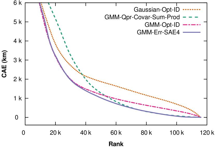
Figure 3: Accuracy of each estimate using selected algorithms, in descending order of CAE.

Figure 3 plots the CAE of each estimate from four key algorithms. These curves are classic long-tail distributions (as are similar ones for Phys. Rev. A50 omitted for brevity); that is, a relatively small number of difficult tweets comprise the bulk of the error. Accordingly, summarizing our results by median instead of mean may be of some value: for example, the median CAE of GMM-Err-SAE4 is 778 km, and its median Phys. Rev. A50 is 83,000 $\text{km}^{2}$ (roughly the size of Kansas or Austria). However, we have elected to focus on reporting means in order to not conceal poor performance on difficult tweets.

It is plausible that different algorithms may perform poorly on different types of test tweets, though we have not explored this; the implication is that selecting different strategies based on properties of the tweet being located may be of value.

5.1.4 Compared to prior work with the Eisenstein data set

Algorithm	SAE
	Mean	Median	$\text{OC}_{\bm{50}}$	n-grams
Hong et al. [17]		373
Eisenstein et al. [11]	845	501
GMM-Opt-ID	870	534	0.50	19
Roller et al. [28]	897	432
Eisenstein et al. [10]	900	494
GMM-Err-SAE6	946	588	0.50	153
GMM-Err-SAE16	954	493	0.36	37
Wing et al. [34]	967	479
GMM-Err-SAE4	985	684	0.55	182

Table 2: Our algorithms compared with previous work, using the dataset from Eisenstein et al. [10]. The n-grams column reports the mean number of n-grams used to locate each test tweet.

Table 2 compares GMM-Opt-ID and GMM-Err-SAE to five competing approaches using data from Eisenstein et al. [10], using mean and median SAE (as these were the only metrics reported).

These data and our own have important differences. First, they are limited to tweets from the United States — thus, we expect lower error here than in our data, which contain tweets from across the globe. Second, these data were created for user location inference, not message location (that is, they are designed for methods which assume users tend to stay near the same location, whereas our model makes no such assumption and thus may be more appropriate when locating messages from unknown users). To adapt them to our message-based algorithms, we concatenate all tweets from each user, treating them as a single message, as in [17]. Finally, the Eisenstein data contain only unigrams from the text field (as we will show, including information from other fields can notably improve results); for comparison, we do the same. This yields 7,580 training and 1,895 test messages (i.e., roughly 380,000 tweets versus 13 million in our data set).

Judged by mean SAE, GMM-Opt-ID surpasses all other approaches except for Eisenstein et al. [11]. Interestingly, the algorithm ranking varies depending on whether mean or median SAE is used — e.g., GMM-Err-SAE16 has lower median SAE than [11] but a higher mean SAE. This trade-off between mean and median SAE also appears in other work – for example, Eisenstein et al. report the best mean SAE but have much higher median SAE [11]. Also, Hong et al. report the best median SAE but do not report mean at all [17].

Examining the results for GMM-Err-SAE sheds light on this discrepancy. We see that as the exponent increases from 4 to 16, the median SAE decreases from 684 km to 493 km. However, calibration suffers rather dramatically: GMM-Err-SAE16 has a quite overconfident $\text{OC}_{50}=0.36$. This is explained in part by its use of fewer n-grams per message (182 for an exponent of 4 versus 37 for exponent 16).

Moreover, to our knowledge, no prior work reports either precision or calibration metrics, making a complete comparison impossible. For example, the better mean SAE of Eisenstein et al. [11] may coincide with worse precision or calibration. These metrics are not unique to our GMM method, and we argue that they are critical to understanding techniques in this space, as the trade-off above demonstrates.

Finally, we speculate that a modest decrease in accuracy may not outweigh the simplicity and scalability of our approach. Specifically in contrast to topic modeling approaches, our learning phase can be trivially parallelized by n-gram.

5.2 RQ2: Training size

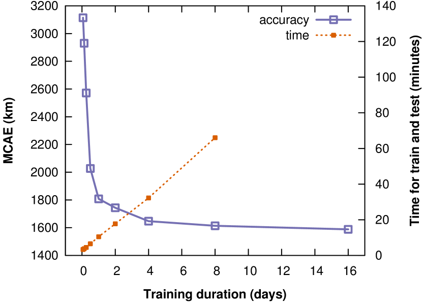
Figure 4: Accuracy of GMM-Err-SAE4 with different amounts of training data, along with the mean time to train and test one model. Each day contains roughly 32,000 training tweets. (The 16-day test was run in a nonstandard configuration and its timing is therefore omitted.)

We evaluated the accuracy of GMM-Err-SAE4 on different training durations, no gap, all fields except user description, and minimum instances of 3. We used a stride of 13 days for performance reasons.

Figure 4 shows our results. The knee of the curve is 1 day of training (i.e., about 30,000 tweets), with error rapidly plateauing and training time increasing as more data are added; accordingly, we use 1 training day in our other experiments.

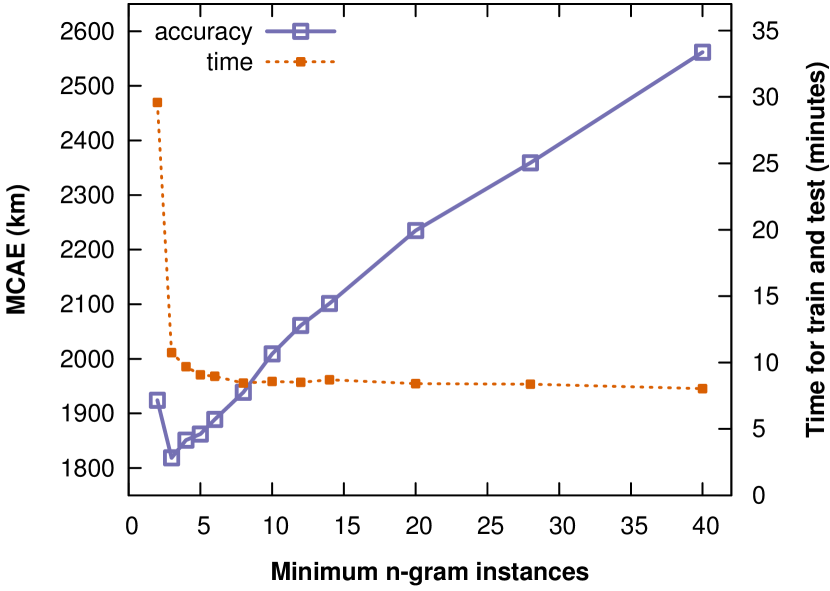
Figure 5: Accuracy and run time of GMM-Err-SAE4 vs. inclusion thresholds for the number of times an n-gram appears in training data.

We also evaluated accuracy when varying minimum instances (the frequency threshold for retaining n-grams), with training days fixed at 1; Figure 5 shows the results. Notably, including n-grams which appear only 3 times in the training set improves accuracy at modest time cost (and thus we use this value in our other experiments). This might be explained in part by the well-known long-tail distribution of word frequencies; that is, while the informativeness of each individual n-gram may be low, the fact that low-frequency words occur in so many tweets can impact overall accuracy. This finding supports Wing & Baldridge’s suggestion [34] that Eisenstein et al. [10] pruned too aggressively by setting this threshold to 40.

5.3 RQ3: Time dependence

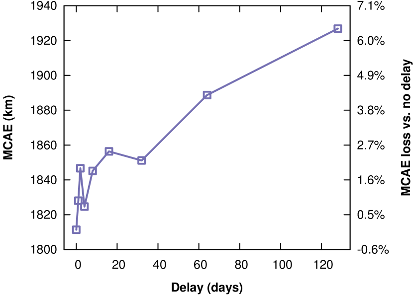
Figure 6: Accuracy of GMM-Err-SAE4 with increasing delay between training and testing.

We evaluated the accuracy of GMM-Err-SAE4 on different temporal gaps between training and testing, holding fixed training duration of 1 day and minimum n-gram instances of 3. Figure 6 summarizes our results. Location inference is surprisingly time-invariant: while error rises linearly with gap duration, it does so slowly – there is only about 6% additional error with a four-month gap. We speculate that this is simply because location-informative n-grams which are time-dependent (e.g., those related to a traveling music festival) are relatively rare.

5.4 RQ4: Location signal source

We wanted to understand which types of content provide useful location information under our algorithm. For example, Figure 1 on the first page illustrates a successful estimate by GMM-Err-SAE4. Recall that this was based almost entirely on the n-grams angeles ca and ca, both from the location field. Table 5.1 in the appendices provides a further snapshot of the algorithm’s output. These hint that, consistent with other methods (e.g., [16]), toponyms provide the most important signals; below, we explore this hypothesis in more detail.

5.4.1 Which fields provide the most value?

One framing of this research question is structural. To measure this, we evaluated GMM-Err-SAE4 on each combination of the five tweet fields, holding fixed training duration at 1 day, gap at zero, and minimum instances at 3. This requires an additional metric: success rate is the fraction of test tweets for which the model can estimate a location (i.e., at least one n-gram in the test tweet is present in the trained model).

Field	Alone		Improvement
	MCAE	success	MCAE	success
user location	2125	65.8%	1255	1.7%
user time zone	2945	76.1%	910	3.0%
tweet text	3855	95.7%	610	7.3%
user description	4482	79.7%	221	3.3%
user language	6143	100.0%	-103	8.5%

Table 3: Value of each field. Alone shows the accuracy and success rate of estimation using that field alone, while Improvement shows the mean improvement when adding a field to each combination of other fields (in both cases, positive indicates improvement). For example, adding user location to some combination of the other four fields will, on average, decrease MCAE by 1,255 km and increase the success rate by 1.7 percentage points.

Rank	Fields					MCAE	success
1	lo	tz	tx		ln	1823	100.0%
2	lo	tz	tx	ds	ln	1826	100.0%
3	lo	tz				1862	87.7%
4	lo	tz	tx			1878	99.2%
5	lo	tz	tx	ds		1908	99.6%
6	lo	tz		ds		2013	94.1%
7	lo	tz		ds	ln	2121	100.0%
8	lo					2125	65.8%
9	lo		tx	ds	ln	2176	100.0%
10	lo	tz			ln	2207	100.0%
11	lo		tx	ds		2274	99.2%
12	lo		tx		ln	2310	100.0%
13	lo		tx			2383	98.0%
14		tz	tx	ds	ln	2492	100.0%
15	lo			ds		2585	88.3%
16		tz	tx	ds		2594	99.4%
17		tz	tx		ln	2617	100.0%
18		tz	tx			2691	98.7%
19	lo			ds	ln	2759	100.0%
20		tz				2945	76.1%
21		tz		ds		2991	91.8%
22		tz		ds	ln	3039	100.0%
23	lo				ln	3253	100.0%
24			tx	ds	ln	3267	100.0%
25			tx	ds		3426	98.8%
26		tz			ln	3496	100.0%
27			tx		ln	3685	100.0%
28			tx			3855	95.7%
29				ds		4482	79.7%
30				ds	ln	4484	100.0%
31					ln	6143	100.0%

Table 4: Accuracy of including different fields. We list each combination of fields, ordered by increasing MCAE.

Table 3 summarizes our results, while Table 4 enumerates each combination. User location and time zone are the most accurate fields, with tweet text and language important for success rate. For example, comparing the first and third rows of Table 4, we see that adding text and language fields to a model that considers only location and timezone fields improves MCAE only slightly (39 km) but improves success rate considerably (by 12.3% to 100.0%). We speculate that while tweet text is a noisier source of evidence than time zone (due to the greater diversity of locations associated with each n-gram), our algorithm is able to combine these sources to increase both accuracy and success rate.

It is also interesting to compare the variant considering only the location field (row 8 of Table 4) with previous work that heuristically matches strings from the location field to gazetteers. Hecht et al. found that 66% of user profiles contain some type of geographic information in their location field [16], which is comparable to the 67% success rate of our model using only location field.

Surprisingly, user description adds no value at all; we speculate that it tends to be redundant with user location.

5.4.2 Which types of n-grams provide the most value?

We also approached this question by content analysis. To do so, from an arbitrarily chosen test of the 58 successful GMM-Err-SAE4 tests, we selected a “good” set of the 400 (or 20%) lowest-CAE tweets, and a “bad” set of the 400 highest-CAE tweets. We further randomly subdivided these sets into 100 training tweets (yielding 162 good n-grams and 457 bad ones) and 300 testing tweets (364 good n-grams and 1,306 bad ones, of which we randomly selected 364).

Two raters independently created categories by examining n-grams from the location and tweet text fields in the training sets. These were merged by discussion into a unified hierarchy. The same raters then independently categorized n-grams from the two fields into this hierarchy, using Wikipedia to confirm potential toponyms and Google Translate for non-English n-grams. Disagreements were again resolved by discussion.

Table 5: Content analysis of n-grams in the location and text fields. For each category, we show the fraction of total weight in all location estimates from n-grams of that category; e.g., 49% of all estimate weight in the good estimates was from n-grams with category city (weights do not add up to 100% because time zone and language fields are not included). Weights that are significantly greater in good estimates than bad (or vice versa) are indicated with a significance code ($\circ$ = 0.1, $\ast$ = 0.05, $\ast\ast$ = 0.01, $\ast$$\ast$$\ast$ = 0.001) determined using a Mann-Whitney U test with Bonferroni correction, the null hypothesis being that the mean weight assigned to a category over all n-grams in the good set is equal to the mean weight for the same category in the bad set. Categories with less than 1.5% weight in both classes are rolled up into other. We also show the top-weighted examples in each category.

Our results are presented in Table 5.1. Indeed, toponyms offer the strongest signal; fully 83% of the n-gram weight in well-located tweets is due to toponyms, including 49% from city names. In contrast, n-grams used for poorly-located tweets tended to be non-toponyms (57%). Notably, languages with geographically compact user bases, such as Dutch, also provided strong signals even for non-toponyms.

These results and those in the previous section offer a key insight into gazetteer-based approaches [13, 16, 26, 30, 32], which favor accuracy over success rate by considering only toponyms. However, our experiments show that both accuracy and success rate are improved by adding non-toponyms, the latter to nearly 100%; for example, compare rows 1 and 8 of Table 4. Further, Table 5.1 shows that 17% of location signal in well-located tweets is not from toponyms.

6 Implications

We propose new judgement criteria for location estimates and specific metrics to compute them. We also propose a simple, scalable method for location inference that is competitive with more complex ones, and we validate this approach using our new criteria on a dataset of tweets that is comprehensive temporally, geographically, and linguistically.

This has implications for both location inference research as well as applications which depend on such inference. In particular, our metrics can help these and related inference domains better balance the trade-off between precision and recall and to reason properly in the presence of uncertainty.

Our results also have implications for privacy. In particular, they suggest that social Internet users wishing to maximize their location privacy should (a) mention toponyms only at state- or country-scale, or perhaps not at all, (b) not use languages with a small geographic footprint, and, for maximal privacy, (c) mention decoy locations. However, if widely adopted, these measures will reduce the utility of Twitter and other social systems for public-good uses such as disease surveillance and response. Our recommendation is that system designers should provide guidance enabling their users to thoughtfully balance these issues.

Future directions include exploring non-gaussian and non-parametric density estimators and improved weighting algorithms (e.g., perhaps those optimizing multiple metrics), as well as ways to combine our approach with others, in order to take advantage of a broader set of location clues. We also plan to incorporate priors such as population density and to compare with human location assessments.

7 Acknowledgments

Susan M. Mniszewski, Geoffrey Fairchild, and other members of our research team provided advice and support. We thank our anonymous reviewers for key guidance and the Twitter users whose content we studied. This work is supported by NIH/NIGMS/MIDAS, grant U01-GM097658-01. Computation was completed using Darwin, a cluster operated by CCS-7 at LANL and funded by the Accelerated Strategic Computing Program; we thank Ryan Braithwaite for his technical assistance. Maps were drawn using Quantum GIS; base map geodata is from Natural Earth. LANL is operated by Los Alamos National Security, LLC for the Department of Energy under contract DE-AC52-06NA25396.

8 Appendix: Mathematical implementations

Table 6: Example output of GMM-Err-SAE4 for an arbitrarily selected test. TZ is the time zone field (with -timeuscanada omitted), while L is the language code. N-grams which collectively form 95% of the estimate weight are listed. CAE is in kilometers, while Phys. Rev. A50 is in square kilometers.

8.1 Metrics

This section details the mathematical implementation of the metrics presented above. To do so, we use the following vocabulary. Let $m$ be a message represented by a binary feature vector of n-grams (i.e., sequences of up to $n$ adjacent tokens; we use $n=2$) $m=\{w_{1}\ldots w_{V}\}$, $w_{j}\in\{0,1\}$. $w_{j}=1$ means that n-gram $w_{j}$ appears in message $m$, and $V$ is the total size of the vocabulary. Let $y\in\mathbbm{R}^{2}$ represent a geographic point (for example, latitude and longitude) somewhere on the surface of the Earth. We represent the true origin of a message as $y^{*}$; given a new message $m$, our goal is to construct a geographic density estimate $f(y|m)$, a function which estimates the probability of each point $y$ being the true origin of $m$.

These implementations are valid for any density estimate $f$, not just gaussian mixture models. Specific types of estimates may require further detail; for GMMs, this is noted below.

CAE depends further on the geodesic distance $d(y,y^{*})$ between the true origin $y^{*}$ and some other point $y$. It can be expressed as:

$$\text{CAE}=\text{E}_{f}[d(y,y^{*})]=\int_{y}d(y,y^{*})f(y|m)\,\mathrm{d}y$$ (1)

As computing this integral is intractable in general, we approximate it using a simple Monte Carlo procedure. First, we generate a random sample of $n$ points from the density $f$, $S=\{y_{1}\ldots y_{n}\}$ ($n=1000$ in our experiments). Using this sample, we compute CAE as follows:

$$\text{CAE}\approx\frac{1}{|S|}\sum_{y\in S}d(y,y^{*})$$ (2)

Note that in this implementation, the weighting has become implicit: points that are more likely according to $f$ are simply more likely to appear in $S$. Thus, if $f$ is a good estimate, most of the samples in $S$ will be near the true origin.

To implement PRA, let $R_{f,\beta}$ be a prediction region such that the probability of $y^{*}$ falling within the geographic region $R$ is its coverage $\beta$. Then, Phys. Rev. Aβ is simply the area of $R$:

$${\rm Phys.~{}Rev.~{}A}{\beta}=\int_{R_{f,\beta}}\!\!\,\mathrm{d}y$$ (3)

As above, we can use a sample of points $S$ from $f$ to construct an approximate version of $R$:

1. Sort $S$ in descending order of likelihood $f(y_{i}|m)$. Let $S_{\beta}$ be the set containing the top $|S|\beta$ sample points.

2. Divide $S_{\beta}$ into approximately convex clusters.

3. For each cluster of points, compute its convex hull, producing a geo-polygon.

4. The union of these hulls is approximately $R_{f,\beta}$, and the area of this set of polygons is approximately Phys. Rev. Aβ.

Finally, recall that $\text{OC}_{\beta}$ for a given estimator and a set of test messages is the fraction of tests where $y^{*}$ was within the prediction region $R_{f,\beta}$. That is, for a set $(y_{1}^{*},y_{2}^{*},...y_{n}^{*})$ of $n$ true message origins:

$$\text{OC}_{\beta}=\frac{1}{n}\sum_{i=1}^{n}\mathbbm{1}[y_{i}^{*}\in R^{i}_{f,\beta}]$$ (4)

We do not explicitly test whether $y^{*}\in R$, because doing so propagates any errors in approximating $R$. Instead, we count how many samples in $S$ have likelihood less than $f(y^{*}|m)$; if this fraction is greater than $\beta$, then $y^{*}$ is (probably) in $R$. Specifically:

$$r(y^{*})=\frac{1}{|S|}\sum_{y\in S}\mathbbm{1}[f(y)<f(y^{*})]$$ (5)

$$\text{OC}_{\beta}\approx\frac{1}{n}\sum_{i=1}^{n}\mathbbm{1}[r(y_{i}^{*})>\beta]$$ (6)

8.2 Gaussian mixture models

As introduced in section “Our Approach”, we construct our location model by training on geographic data consisting of a set $D$ of $n$ (message, true origin) pairs extracted from our database of geotagged tweets; i.e., $D=\{(m_{i},y^{*}_{i})\}_{i=1}^{n}$. For each n-gram $w_{j}$, we fit a gaussian mixture model $g(y|w_{j})$ based on examples in $D$. Then, to estimate the origin location of a new message $m$, we combine the mixture models for all n-grams in $m$ into a new density $f(y|m)$. These steps are detailed below.

We estimate $g$ for each (sufficiently frequent) n-gram $w_{j}$ in $D$ as follows. First, we gather the set of true origins of all messages containing $w_{j}$, and then we fit a gaussian mixture model of $r$ components to represent the density of these points:

$$g(y|w_{j})=\sum_{k=1}^{r}\pi_{k}^{j}\,\mathcal{N}(y|\mu_{k}^{j},S_{k}^{j})$$ (7)

where $\pi^{j}=\{\pi^{j}_{1}\ldots\pi^{j}_{r}\}$ is a vector of mixture weights and $\mathcal{N}$ is the normal density function with mean $\mu^{j}_{k}$ and covariance $S^{j}_{k}$. We refer to $g(y|w_{j})$ as an n-gram density.

We fit $\pi$ and $S$ independently for each n-gram using the expectation maximization algorithm, as implemented in the Python package scikit-learn [27].

Choosing the number of components $r$ is a well-studied problem. While Dirichlet process mixtures [24] are a common solution, they can scale poorly. For simplicity, we instead investigated a number of heuristic approaches from the literature [23]; in our case, $r=\min(m,\log(n)/2)$ worked well, where $n$ is the number of points to be clustered, and $m$ is a parameter. We use this heuristic with $m=20$ in all experiments.

Next, to estimate the origin of a new message $m$, we gather the available densities $g$ for each n-gram in $m$ (i.e., some n-grams may appear in $m$ but not in sufficient quantity in $D$). We combine these n-gram densities into a mixture of GMMs:

$$f(y|m) =\sum_{w_{j}\in m}\delta_{j}g(y|w_{j})=\sum_{w_{j}\in m}\delta_{j}\sum_{k=1}^{r}\pi_{k}^{j}\,\mathcal{N}(y|\mu_{k}^{j},S_{k}^{j})$$ (8)

where $\delta=\{\delta_{1}\ldots\delta_{V}\}$ are the n-gram mixture weights associated with each n-gram density $g$. We refer to $f(y|m)$ as a message density.

A mixture of GMMs can be implemented as a single GMM by multiplying $\delta_{j}$ by $\pi^{j}_{k}$ for all $j,k$ and renormalizing so that the mixture weights sum to 1. Thus, Equation 8 can be rewritten:

$$f(y|m)=\sum_{w_{j}\in m}\sum_{k=1}^{r}\tau_{k}^{j}\,\mathcal{N}(y|\mu_{k}^{j},S_{k}^{j})$$ (9)

where $\tau_{k}^{j}=\delta_{j}\pi_{k}^{j}/\sum_{j,k}\delta_{j}\pi_{k}^{j}$.

We can now compute all four metrics. CAE and $\text{OC}_{\beta}$ require no additional treatment. To compute SAE, we distill $f(y|m)$ into a single point estimate by the weighted average of its component means: $\hat{y}=\sum_{w_{j}\in m}\sum_{k=1}^{r}\tau_{k}^{j}\mu_{k}^{j}$. Computing Phys. Rev. Aβ requires dividing $S_{\beta}$ into convex clusters; we do so by assigning each point in $S$ to its most probable gaussian in $f$.

The next two sections describe methods to set the n-gram mixture weights $\delta_{j}$.

8.3 Setting $\delta_{j}$ weights by inverse error

Mathematically, the inverse error approach introduced above can be framed as a non-iterative optimization problem. Specifically, we set $\delta$ by fitting a multinomial distribution to the observed error distribution. Let $e_{ij}\in\mathbbm{R}_{\geq 0}$ be the error incurred by n-gram density $g(y|w_{j})$ for message $m_{i}$; in our implementation, we use SAE as $e_{ij}$ for performance reasons (results with CAE are comparable). Let $e_{j}$ be the average error of n-gram $w_{j}$: $e_{j}=\frac{1}{N_{j}}\sum_{i=1}^{N_{j}}e_{ij}$, where $N_{j}$ is the number of messages containing $w_{j}$. We introduce a model parameter $\alpha$, which places a non-linear (exponential) penalty on error terms $e_{j}$. The problem is to minimize the negative log likelihood, with constraints that ensure $\delta$ is a probability distribution:

$$\delta^{*}\leftarrow \mathop{\rm argmin}_{\delta}-\log\prod_{j}\delta_{j}^{\frac{1}{e_{j}^{\alpha}}}$$ (10)

$$\text{s.t. }\sum_{j}\delta_{j}=1\text{ and }\delta_{j}\geq 0\text{ }\forall j$$ (11)

This objective can be minimized analytically. While the inequality constraints in Equation 11 will be satisfied implicitly, we express the equality constraints using a Lagrangian:

$$L(\delta,\lambda) =-\log\prod_{j}\delta_{j}^{\frac{1}{e_{j}^{\alpha}}}+\lambda\left(\sum_{j}\delta_{j}-1\right)$$ (12)

$$=-\sum_{j}\frac{1}{e_{j}^{\alpha}}\log\delta_{j}+\lambda\left(\sum_{j}\delta_{j}-1\right)$$ (13)

Taking the partial derivative with respect to $\delta_{k}$ and setting to 0 results in:

$$\frac{\partial L}{\partial\delta_{k}} =-\frac{1}{e_{k}^{\alpha}\delta_{k}}+\lambda=0\text{ }\forall k$$ (14)

$$=-\frac{1}{e_{k}^{\alpha}}+\lambda\delta_{k}=0\text{ }\forall k$$ (15)

$$\frac{\partial L}{\partial\delta} =-\sum_{k}\frac{1}{e_{k}^{\alpha}}+\lambda\sum_{k}\delta_{k}=0$$ (16)

The equality constraint lets us substitute $\sum_{k}\delta_{k}=1$ in Equation 16. Solving for $\lambda$ yields:

$$\lambda=\sum_{k}\frac{1}{e_{k}^{\alpha}}$$ (17)

Plugging this into 14 and solving for $\delta_{k}$ results in:

$$\delta_{k}=\frac{\frac{1}{e_{k}^{\alpha}}}{\sum_{k}\frac{1}{e_{k}^{\alpha}}}$$ (18)

This brings us full circle to the intuitive result above: that the weight of an n-gram is proportional to its average error.

8.4 Setting $\delta_{j}$ weights by optimization

This section details the data-driven optimization algorithm introduced above. We tag each n-gram density function with a feature vector. This vector contains the ID of the n-gram density function, the quality properties, or both of these. For example, the feature vector for the n-gram dallas might be $\{\text{id}=1234,\text{variance}=0.56,\text{BIC}=0.01,...\}$. We denote the feature vector for n-gram $w_{j}$ as $\phi(w_{j})$, with elements $\phi_{k}(w_{j})\in\phi(w_{j})$.

This feature vector is paired with a corresponding real-valued parameter vector $\theta=\{\theta_{1},\ldots,\theta_{p}\}$ setting the weight of each feature. The vectors $\theta$ and $\phi$ are passed through the logistic function to ensure the final weights $\delta$ are in the interval [0,1]:

$$\delta_{j}^{\theta}=\frac{1}{1+e^{-\sum_{k=1}^{p}\phi_{k}(w_{j})\theta_{k}}}$$ (19)

The goal of this approach is to assign values to $\theta$ such that properties that are predictive of low-error n-grams have high weight (equivalently, so that these n-grams have large $\delta_{j}^{\theta}$). This is accomplished by minimizing an error function (built atop the same SAE-based $e_{ij}$ as the previous method):

$$\theta^{*} \leftarrow\mathop{\rm argmin}_{\theta}\sum_{i=1}^{|D|}\frac{\sum_{w_{j}\in m_{i}}e_{ij}\delta_{j}^{\theta}}{\sum_{w_{j}\in m_{i}}\delta_{j}^{\theta}}$$ (20)

After optimizing $\theta$, we assign $\delta^{*}=\delta^{\theta^{*}}\!$. The numerator in Equation 20 computes the sum of mixture weights for each n-gram density weighted by its error; the denominator sums mixture weights to ensure that the objective function is not trivially minimized by setting $\delta_{j}^{\theta}$ to 0 for all $j$. Thus, to minimize Equation 20, n-gram densities with large errors must be assigned small mixture weights.

Before minimizing, we first augment the error function in Equation 20 with a regularization term:

$$\Phi(D,\theta)=\sum_{i=1}^{|D|}\frac{\sum_{w_{j}\in m_{i}}e_{ij}\delta_{j}^{\theta}}{\sum_{w_{j}\in m_{i}}\delta_{j}^{\theta}}+\frac{\lambda}{2}\|\theta\|^{2}$$ (21)

The extra term is an $\ell_{2}$-regularizer to encourage small values of $\theta$ to reduce overfitting; we set $\lambda=1$ in our experiments.

We minimize Equation 21 using gradient descent. For brevity, let $n_{ij}=\sum_{w_{j}\in m_{i}}e_{ij}\delta_{j}^{\theta}$ and $d_{ij}=\sum_{w_{j}\in m_{i}}\delta_{j}^{\theta}$ be the numerator and denominator terms from Equation 21. Then, the gradient of Equation 21 with respect to $\theta_{k}$ is

$$\frac{\partial\Phi}{\partial\theta_{k}}=\sum_{i=1}^{|D|}\sum_{w_{j}\in m_{i}}\frac{-\phi_{k}(w_{j})\delta_{j}^{\theta}(1-\delta_{j}^{\theta})(e_{ij}d_{ij}-n_{ij})}{d_{ij}^{2}}+\lambda\theta_{k}$$ (22)

We set Equation 22 to 0 and solve for $\theta$ using L-BFGS as implemented in the SciPy Python package [18]. (Note that by decomposing the objective function by n-grams, we need only compute the error metrics $e_{ij}$ once prior to optimization.) Once $\theta$ is set, we then find $\delta$ according to Equation 19 and use these values to find the message density in Equation 8.

9 Appendix: Tokenization algorithm

This section details our algorithm to convert a text string into a sequence of n-grams, used to tokenize the message text, user description, and user location fields into bigrams (i.e., $n=2$).

1. Split the string into candidate tokens, each consisting of a sequence of characters with the same Unicode category and script. Candidates not of the letter category are discarded, and letters are converted to lower-case. For example, the string “Can’t wait for 私の” becomes five candidate tokens: can, t, wait, for, and 私の.

2. Candidates in certain scripts are discarded either because they do not separate words with a delimiter (Thai, Lao, Khmer, and Myanmar, all of which have very low usage on Twitter) or may not really be letters (Common, Inherited). Such scripts pose tokenization difficulties which we leave for future work.

3. Candidates in the scripts Han, Hiragana, and Katakana are assumed to be Japanese and are further subdivided using the TinySegmenter algorithm [15]. (We ignore the possibility that text in these scripts might be Chinese, because that language has very low usage on Twitter.) This step would split 私の into 私 and の.

4. Create n-grams from adjacent tokens. Thus, the final tokenization of the example for $n=2$ would be: can, t, wait, for, 私, の, can t, t wait, wait for, for 私, and 私 の.

10 Appendix: Results of pilot experiments

This section describes briefly three directions we explored but did not pursue in detail because they seemed to be of limited potential value.

• Unifying fields. Ignoring field boundaries slightly reduced accuracy, so we maintain these boundaries (i.e., the same n-gram appearing in different fields is treated as multiple, separate n-grams).

• Head trim. We tried sorting n-grams by frequency and removing various fractions of the most frequent n-grams. In some cases, this yielded a slightly better MCAE but also slightly reduced the success rate; therefore, we retain common n-grams.

• Map projection. We tried plate carrée (i.e., WGS84 longitude and latitude used as planar X and Y coordinates), Miller, and Mollweide projections. We found no consistent difference with our error- and optimization-based algorithms, though some others displayed variation in MPRA. Because this did not affect our results, we used plate carrée for all experiments, but future work should explore exactly when and why map projection matters.

References

- [1] H. Akaike. A new look at the statistical model identification. Automatic Control, 19(6):716–723, 1974. 10.1109/TAC.1974.1100705.
- [2] D. M. Blei and others. Latent Dirichlet allocation. Machine Learning Research, 3:993–1022, 2003. http://dl.acm.org/citation.cfm?id=944937.
- [3] L. D. Brown et al. Confidence intervals for a binomial proportion and asymptotic expansions. Annals of Statistics, 30(1), 2002. 10.1214/aos/1015362189.
- [4] S. Chandra et al. Estimating Twitter user location using social interactions – A content based approach. In Proc. Privacy, Security, Risk and Trust (PASSAT), 2011. 10.1109/PASSAT/SocialCom.2011.120.
- [5] H. Chang et al. @Phillies tweeting from Philly? Predicting Twitter user locations with spatial word usage. In Proc. Advances in Social Networks Analysis and Mining (ASONAM), 2012. 10.1109/ASONAM.2012.29.
- [6] Z. Cheng et al. You are where you tweet: A content-based approach to geo-locating Twitter users. In Proc. Information and Knowledge Management (CIKM), 2010. 10.1145/1871437.1871535.
- [7] E. Cho et al. Friendship and mobility: User movement in location-based social networks. In Proc. Knowledge Discovery and Data Mining (KDD), 2011. 10.1145/2020408.2020579.
- [8] C. A. Davis Jr. et al. Inferring the location of Twitter messages based on user relationships. Transactions in GIS, 15(6), 2011. 10.1111/j.1467-9671.2011.01297.x.
- [9] M. Dredze. How social media will change public health. Intelligent Systems, 27(4):81–84, 2012. 10.1109/MIS.2012.76.
- [10] J. Eisenstein et al. A latent variable model for geographic lexical variation. In Proc. Empirical Methods in Natural Language Processing, 2010. http://dl.acm.org/citation.cfm?id=1870782.
- [11] J. Eisenstein et al. Sparse additive generative models of text. In Proc. Machine Learning (ICML), 2011. http://www.icml-2011.org/papers/534˙icmlpaper.pdf.
- [12] S. Geisser. Predictive Inference: An Introduction. Chapman and Hall, 1993.
- [13] J. Gelernter and N. Mushegian. Geo-parsing messages from microtext. Transactions in GIS, 15(6):753–773, 2011. 10.1111/j.1467-9671.2011.01294.x.
- [14] M. C. González et al. Understanding individual human mobility patterns. Nature, 453(7196):779–782, 2008. 10.1038/nature06958.
- [15] M. Hagiwara. TinySegmenter in Python. http://lilyx.net/tinysegmenter-in-python/.
- [16] B. Hecht et al. Tweets from Justin Bieber’s heart: The dynamics of the location field in user profiles. In Proc. CHI, 2011. 10.1145/1978942.1978976.
- [17] L. Hong et al. Discovering geographical topics in the Twitter stream. In Proc. WWW, 2012. 10.1145/2187836.2187940.
- [18] E. Jones et al. SciPy: Open source scientific tools for Python, 2001. http://www.scipy.org.
- [19] S. Kinsella et al. “I’m eating a sandwich in Glasgow”: Modeling locations with Tweets. In Proc. Workshop on Search and Mining User-Generated Content (SMUC), 2011. 10.1145/2065023.2065039.
- [20] J. Mahmud et al. Where is this Tweet from? Inferring home locations of Twitter users. In Proc. ICWSM, 2012. http://www.aaai.org/ocs/index.php/ICWSM/ICWSM12/paper/viewFile/4605/5045.
- [21] S. McClendon and A. C. Robinson. Leveraging geospatially-oriented social media communications in disaster response. In Proc. Information Systems for Crisis Response and Management (ISCRAM), 2012. http://iscramlive.org/ISCRAM2012/proceedings/136.pdf.
- [22] G. McLachlan and D. Peel. Finite Mixture Models. Wiley & Sons, 2005. 10.1002/0471721182.
- [23] G. W. Milligan and M. C. Cooper. An examination of procedures for determining the number of clusters in a data set. Psychometrika, 50(2):159–179, 1985. 10.1007/BF02294245.
- [24] R. M. Neal. Markov chain sampling methods for Dirichlet process mixture models. Computational and Graphical Statistics, 9(2), 2000. 10.2307/1390653.
- [25] N. O’Hare and V. Murdock. Modeling locations with social media. Information Retrieval, 16(1):1–33, 2012. 10.1007/s10791-012-9195-y.
- [26] S. Paradesi. Geotagging tweets using their content. In Proc. Florida Artificial Intelligence Research Society, 2011. http://www.aaai.org/ocs/index.php/FLAIRS/FLAIRS11/paper/viewFile/2617/3058.
- [27] F. Pedregosa et al. Scikit-learn: Machine learning in Python. Machine Learning Research, 12:2825–2830, 2011. http://dl.acm.org/citation.cfm?id=2078195.
- [28] S. Roller et al. Supervised text-based geolocation using language models on an adaptive grid. In Proc. Empirical Methods in Natural Language Processing and Computational Natural Language Learning (EMNLP-CoNLL), 2012. http://dl.acm.org/citation.cfm?id=2391120.
- [29] N. Savage. Twitter as medium and message. CACM, 54(3):18–20, 2011. 10.1145/1897852.1897860.
- [30] A. Schulz et al. A multi-indicator approach for geolocalization of tweets. In Proc. ICWSM, 2013.
- [31] G. Schwarz. Estimating the dimension of a model. Annals of Statistics, 6(2):461–464, 1978. 10.1214/aos/1176344136.
- [32] G. Valkanas and D. Gunopulos. Location extraction from social networks with commodity software and online data. In Proc. Data Mining Workshops (ICDMW), 2012. 10.1109/ICDMW.2012.128.
- [33] C. Wang et al. Mining geographic knowledge using location aware topic model. In Proc. Workshop on Geographical Information Retrieval (GIR), 2007. 10.1145/1316948.1316967.
- [34] B. Wing and J. Baldridge. Simple supervised document geolocation with geodesic grids. In Proc. Association for Computational Linguistics (ACL), 2011. https://www.aclweb.org/anthology-new/P/P11/P11-1096.pdf.