Abstract

In this paper, we discuss the computation of first-passage moments of a time-homogeneous semi-Markov process (SMP) with finite state space to certain of its states that possess the property of universal accessibility (UA). A UA state is one which is accessible from any other state of the SMP, but which may or may not connect back to one or more other states. An important characteristic of UA is that it is the state-level version of the oft-invoked process-level property of irreducibility. We adapt existing results for irreducible SMPs to the derivation of an analytical matrix expression for the first passage moments to a single UA state of the SMP. In addition, consistent estimators for these first passage moments are given.

First Passage Moments of Finite-State Semi-Markov Processes

1 Introduction

The first passage distribution of a discrete-state stochastic model such as a Markov or semi-Markov process is a fundamental quantity of interest. Results for the first passage distribution of a regular Markov process, which is commonly defined as irreducible and aperiodic, are detailed in the classical monograph by Kemeny and Snell [16] and were subsequently developed by Hunter [12, 14]. Nevertheless, many multi-state models that arise in practice use reducible models. One of the early examples of a SMP model that incorporates transient and absorbing states comes from clinical management science [33]. Recent applications from reliability and survival analysis that require transient and absorbing states include a nuclear pipeline rupture model of Veeramany, et al. [32] and the reliability-risk model for credit score ratings of D’Amico, et al. [8]. In such applications, absorbing states are commonly used to indicate failure while transient states arise from degradation levels that may only be visited once.

Modeling applicability of multistate jump models may be further extended by considering the semi-Markov process (SMP), which generalizes the continuous-time Markov chain. Since the seminal works of Levy [22, 23] and Smith [31], semi-Markov processes (SMPs) have been utilized as a framework for a wide variety of applications within the scientific literature. Much of the interest is due to the fact that the SMP relaxes the assumption of exponential sojourn times, which is not always appropriate, while retaining the memoryless characteristic of a Markov chain at the transition epochs. An area of study most frequently associated with SMPs is that of survival analysis and reliability, for which the definitive reference is [3], and which has been continued by the likes of [1, 5, 24] and others. Of special note are the areas of semi-Markov decision processes and $PH$-distributions [17, 35], often used in reliability, but which also appear in the context of SMP first passage moments, as in [36]. Numerical algorithms for the efficient calculation of first-passage moments have also been studied (e.g., [13]), and important developments since [16] are presented in the survey paper by Hunter [14]. Other areas that have seen the application of SMP models are DNA analysis [2], queueing theory [19, 26], finance [15], artificial intelligence [35], and transportation [4, 21], to name but a few.

Explicit time-domain formulas for the first two moments of the first passage distribution of a irreducible ergodic SMP with a finite state space have long been known. Pyke [27, 28] inverted Laplace-Stieltjes transform matrices under restrictive non-singularity conditions in order to derive the first and second moments. Hunter [10] repeated this analysis by means of Markov renewal theory, and then solved for the matrix of first passage moments $\bm{M}$ of the SMP through multiplication of the matrix $\bm{I}-\bm{P}$ by a generalized inverse, where $\bm{P}$ is the irreducible transition probability matrix of the embedded discrete time Markov chain. Hunter [12] further demonstrates that $\bm{M}$ may be found using any generalized inverse $\bm{G}$ for $\bm{I}-\bm{P}$. This criterion directly relates to the main result of this paper via the action of a specific generalized inverse on the irreducible partition of the transition matrix of the embedded DTMC. Although the role of the fundamental matrix of the embedded DTMC in solving the problem of finding the first passage moments was recognized since at least Kemeny and Snell [16], it was Hunter [10] that recognized its importance by proving that the fundamental matrix is a particular generalized inverse for $\bm{I}-\bm{P}$. Some years later, Yao [34] was able to use a generalized inverse to find all moments of first passage for irreducible processes. Zhang and Hou [36] likewise employed a generalized inverse method in order to derive exact first passage moments for SMPs with phase- ($PH$-)distributed sojourn times between states, thus capitalizing on the robust interest in the reliability community for these somewhat exponential-like statistical distributions.

In this article, we derive the formulae for first passage moments in SMPs with finite state space. These processes can be reducible and/or periodic, the only restriction we impose is that the final state of interest in the first passage is universally accessible (UA). UA states are those that are accessible from each and every other state of the SMP. It turns out that the UA-focused method is less involved than earlier methods which, in addition to requiring the g-inverse-rendered fundamental matrix, also involves the simultaneous computation of all first passage times in an irreducible process. The proposed approach requires a generous application of linear algebra, namely the Perron-Frobenius theorem generalized to reducible matrices (and hence reducible processes) in order to arrive at the existence of the reduced fundamental matrix. For further details on the Perron-Frobenius theorem, and spectral theory in general, see [9].

The remainder of the paper will proceed as follows. In Section 2, we define notation, terminology, and assumptions that guide the remainder of the discourse. In section 3, we discuss known results for irreducible processes, and hence essential classes in a general SMP. We then present the main result in Section 4, which is the derivation of the formula for the first passage moments under the condition of universal accessibility. Finally, in Section 5, we present a method for estimating the first passage moments of SMPs and a brief example.

2 Notation and Basic Definitions

In this section we introduce the the notation used in this paper. A boldface symbol without indices refers to a matrix (e.g., $\textbf{F}(t)$ is a matrix with elements $F_{{}_{ij}}(t)$ in the $i$th row and $j$th column). We will sometimes drop the function argument for simplicity’s sake; e.g., $\textbf{F}=\textbf{F}(t)$. In the usual way, we define the Dirac-$\delta$ function as

$$\delta_{{}_{ij}}=\left\{\begin{array}[]{l l}0&\quad\text{if $i\neq j$}\\ 1&\quad\text{if $i=j$}\\ \end{array}\right.$$

In addition, we will specify that the $k$-dimensional square matrices $\bm{I}$ and $\bm{E}$ denote the identity matrix and the matrix whose entries consist of ones, respectively. Finally, the matrix binary operator ‘$\circ$’ denotes Hadamard (element-wise) multiplication; i.e.

$$\big{[}\textbf{A}\circ\textbf{B}\big{]}_{{}_{ij}}=a_{{}_{ij}}b_{{}_{ij}}.$$

We introduce semi-Markov processes roughly following the development in [13]. Consider a Markov renewal process (MRP) $\{(X_{n},T_{n}),n\geq 0\}$ with finite state space $\mathcal{S}=\{1,2,\dots,k\}$ and semi-Markov kernel $\bm{Q}(t)=[Q_{{}_{ij}}(t)]$, where

$$Q_{{}_{ij}}(t)=Pr(X_{n+1}=j,T_{n+1}-T_{n}\leq t|X_{n}=i)$$

and $i,j\in\mathcal{S}$. $X_{n}$ represents the state of the process after the $n^{\text{th}}$ transition and $T_{n}$ is the time at which the $n^{\text{th}}$ transition occurred.

Define $\bm{P}$ to be the matrix of transition probabilities composed of

$$p_{{}_{ij}}\equiv Q_{{}_{ij}}(+\infty)=Pr(X_{n+1}=j|X_{n}=i).$$

Also let $\bm{F}(t)$ be the matrix of cumulative distribution functions (CDFs)

$$F_{{}_{ij}}(t)\equiv Pr(T_{n+1}-T_{n}\leq t|X_{n}=i,X_{n+1}=j),$$

thus $Q_{{}_{ij}}(t)=p_{{}_{ij}}F_{{}_{ij}}(t)$ or $\bm{Q}\equiv\bm{P}\circ\bm{F}$. Additionally, define

$$n_{{}_{ij}}^{(r)}\equiv\int_{0}^{\infty}t^{r}dF_{{}_{ij}}(t)$$

for $r\in\mathbb{N}$. $n_{{}_{ij}}^{(r)}$ is the $r^{\text{th}}$ moment of the process sojourn time in state $i$ when transitioning next to state $j$. Finally, let $\bm{N}^{(r)}\equiv[n_{{}_{ij}}^{(r)}]$, with $\bm{N}\equiv\bm{N}^{(1)}$ and $n_{{}_{ij}}^{(1)}\equiv n_{{}_{ij}}$. In this article we require $0<n_{{}_{ij}}<\infty$ for all $i$ and $j$, when $p_{ij}>0$.

Let $\zeta\equiv\{X(t):t\geq 0\}$, where $X(t)\equiv X_{n}$ for $t\in[T_{n},T_{n+1})$. Thus $\zeta$ is a regular time-homogeneous SMP as a consequence of the above definitions.

We next address the properties of communication between the states of $\zeta$. In [7], the notion of connectedness between states is given in terms of the underlying counting process of the MRP $\left\{\bm{W}(t)\,:\,t>0\right\}$, where $\bm{W}(t)=[W_{j}(t)]_{j\in S}$ is a vector-valued random variable for which $W_{j}(t)$ counts the number of times during the interval $(0,\,t]$ that $\zeta$ transitions into state $j$. If one then defines the $k\times k$ matrix $\bm{\Psi}(t)$ in terms of its $ij^{\text{th}}$ entry

$$\Psi_{ij}(t)=Pr\left(W_{j}(t)>0\,\middle|\,X(0)=i\right),$$

then, the accessibility of state $j$ from state $i$, that is, $i\to j$, is equivalent to the statement that

$$\Psi_{ij}(\infty)=\lim_{t\to\infty}\Psi_{ij}(t)>0.$$

In other words, the process $\zeta$ will transition from state $i$ to state $j$ in finite time with probability 1. Communication between a pair of states $i$ and $j$, that is, $i\to j$ and $j\to i$, will be denoted as $i\leftrightarrow j$. If we specify that reflexivity holds for $\leftrightarrow$, that is, every state communicates with itself, it can be shown that communication is an equivalence relation in the state space $S$. Thus, it follows that $S$ is the disjoint union $S=S_{1}\cup S_{2}\cup\dots\cup S_{K}$ of some number $K$ of essential classes of states whose members communicate exclusively within the class. If there exists only one essential class for $\zeta$, then we say that $\zeta$ is irreducible. On the other extreme, any state that is the sole member of an essential class falls into one of the following categories:

1. Strict Transience: There is no possibility of returning to the state once the process leaves it. In other words, if state $j$ is strictly transient, then

   $$\Psi_{jj}(+\infty)=0.$$

2. Absorption: A state $j$ is called absorbing if it can only return to itself; that is

   $$\Psi_{ji}(+\infty)=0,\quad\Psi_{jj}(+\infty)=1,\quad i\neq j.$$

The presence of some $\Psi_{ij}(+\infty)\in(0,\,1)$ indicates that there is some state $i^{\prime}\in S$ for which $i\to i^{\prime}$, but $i^{\prime}\nrightarrow j$ ($i^{\prime}$ may even be absorbing). Furthermore, we note that the condition $\Psi_{ii}(+\infty)\in(0,\,1)$, may be denoted as non-strict transience of the state $i$. Finally, if $\Psi_{ii}(+\infty)=1$, then a return to state $i$ is inevitable, and so we must have recurrence of the state $i$.

This classification of states into recurrent and transient states suggests an arrangement of the matrix $\Psi(+\infty)$ in which the component blocks are organized according to the normal form $\bm{P}_{N}$ of the reducible probability matrix $\bm{P}$ of the embedded DTMC, which appears as

$$\bm{P}_{N}\sim\bm{\Phi}\bm{P}\bm{\Phi}^{-1}=\left(\begin{array}[]{cccc|cccc}\bm{P}_{11}&\bm{P}_{12}&\cdots&\bm{P}_{1r}&\bm{P}_{1,r+1}&\bm{P}_{1,r+2}&\cdots&\bm{P}_{1k}\\ \bm{0}&\bm{P}_{22}&\cdots&\bm{P}_{2r}&\bm{P}_{2,r+1}&\bm{P}_{2,r+2}&\cdots&\bm{P}_{2k}\\ \vdots&&\ddots&\vdots&\vdots&\vdots&\ddots&\vdots\\ \bm{0}&\bm{0}&\cdots&\bm{P}_{rr}&\bm{P}_{r,r+1}&\bm{P}_{r,r+2}&\cdots&\bm{P}_{rk}\\ \hline\cr\bm{0}&\bm{0}&\cdots&\bm{0}&\bm{P}_{r+1,r+1}&\bm{0}&\cdots&\bm{0}\\ \bm{0}&\bm{0}&\cdots&\bm{0}&\bm{0}&\bm{P}_{r+2,r+2}&\cdots&\bm{0}\\ \vdots&\vdots&\ddots&\vdots&\vdots&&\ddots&\vdots\\ \bm{0}&\bm{0}&\cdots&\bm{0}&\bm{0}&\bm{0}&\cdots&\bm{P}_{kk}\\ \end{array}\right)$$ (1)

where $\bm{\Phi}$ is a permutation matrix. The first $r$ blocks along the diagonal correspond to essential classes of transient states (both strict and non-strict) while the remaining $k-r$ blocks correspond to the recurrent states.

With the relationship between the entries of $\Psi(+\infty)$ and the state properties of $\zeta$ having been established, we next introduce yet another state-level characteristic that is crucial to determining pairs of states for which it is appropriate to compute a first passage moment.

Definition 2.1.

Let $\zeta$ be a SMP with state space $\mathcal{S}$. State $j^{*}\in\mathcal{S}$ is said to be universally accessible (UA) if, for every $i\in\mathcal{S}$, we have $\Psi_{ij^{*}}(+\infty)=1$.

The definition is strong in the sense that, while it is necessary that $i\to j^{*}$ for a UA state $j^{*}$, it is not sufficient. In other words, we must achieve certainty with probability 1 that a process starting in any $i\in S$ must end up in $j^{*}$ in a finite period of time. As a matter of terminology, we shall refer to a state $j^{*}$ for which some entries $0\leq\Psi_{ij}(+\infty)<1$ as sub-UA.

It is often convenient to refer to the arrangement of states in a SMP in graph-theoretic terms. A directed graph, or digraph, associated to $\bm{A}=[a_{ij}]$, denoted $\mathcal{G}(\bm{A})$ is a grouping of nodes (states) connected by vertices in the set $V(\mathcal{G}(\bm{A}))=\{1,2,\dots,k\}$ such that the directed arc, or edge, $(i,j)$ exists if and only if $a_{ij}>0$. $\mathcal{G}(\bm{A})$ is said to be strongly connected if, for each ordered pair $i,j\in V(\mathcal{G}(\bm{A}))$, there exists a (directed) path in $\mathcal{G}(\bm{A})$ from $i$ to $j$. In either case of there being an edge or directed path from $i$ to $j$, the implication is clearly $i\rightarrow j$. The final connection between irreducibility and connectedness is made in the following Proposition:

Proposition 2.1.

Let $\bm{A}$ be a nonnegative square matrix. $\bm{A}$ is irreducible if and only if $\mathcal{G}(\bm{A})$ is strongly connected.

Proof.

See Shao [30]. ∎

We conclude the section with a Proposition that demonstrates the significance of the UA state property, which we assert that, even if it is not greater than that of irreducibility, it is evinced at a more fundamental level:

Proposition 2.2.

A SMP $\{X(t):t\geq 0\}$ with finite state space $\mathcal{S}$ is irreducible if and only if every $j\in\mathcal{S}$ is UA.

The property of a state being UA is, in a sense, the minimal requirement for the existence of a vector of finite first-passage moments for that state.

3 First Passage Times in an Irreducible SMP

We next address known results for the first passage time moments of an irreducible SMP, that is, an SMP for which $\Psi(+\infty)=\bm{E}$ We may select an arbitrary state $j\in S$ for which we define the random variable

$$Y_{{}_{j}}=\inf\{t\geq T_{1}:X(0)=i,\,X(t)=j\},\,j\in\mathcal{S},$$

where $T_{1}>0$ is the time of the first transition. Random variable $Y_{j}$ may be described as the time of first passage from an initial state $i$ to state $j$ if $i\neq j$, and the time of first return to $j$ otherwise. The distribution function $G_{ij}(t)$ of first passage, conditioned on being in the initial state $i\in\mathcal{S}$, is defined as

$$G_{{}_{ij}}(t)=Pr\left(Y_{{}_{j}}\leq t\,\middle|\,X(0)=i\right),$$

and for which the corresponding $r^{\text{th}}$ moments $m_{{}_{ij}}^{(r)}$, $r\geq 1$, if they exist, are given by

$$m_{{}_{ij}}^{(r)}\equiv\int_{0}^{\infty}t^{r}dG_{ij}(t)=E\left[Y_{{}_{j}}^{r}\,\middle|\,X(0)=i\right].$$

We thus define $\bm{G}(t)$ and $\bm{M}^{(r)}=\left[m_{{}_{ij}}^{(r)}\right]$ to be the matrices of first passage cumulative distribution functions and $r^{\text{th}}$ moments, respectively.

As stated in Proposition 5.15 of [29, pg104] and Lemma 4.1 of [36], the moments of first passage for an irreducible SMP may be computed as the finite solution to the systems of equations given by

$$m_{ij} \equiv m_{{}_{ij}}^{(1)}=\sum_{l=1}^{k}p_{{}_{il}}\left[\left(1-\delta_{{}_{lj}}\right)m_{{}_{lj}}+m_{{}_{il}}\right]$$ (2)

$$m_{{}_{ij}}^{(r)} =\sum_{l=1}^{k}p_{{}_{il}}m_{{}_{il}}^{(r)}+\sum_{s=1}^{r}\binom{r}{s}\left[\sum_{l\neq j}p_{{}_{il}}e^{(r-s)}_{{}_{il}}m_{{}_{lj}}^{(s)}\right],\qquad r\geq 2.$$ (3)

One or both of these formulae can also be found in [10], [11], and [13] and are well known in the literature. Clearly, a necessary condition for $m^{(r)}_{{}_{ij}}<+\infty$ is that $i\rightarrow j$, which is certainly true if the SMP is irreducible. In contrast, we observe that $G_{{}_{ij}}(+\infty)<1$ (and $m_{{}_{ij}}=+\infty$) might occur for a pair of states $i,\,j\in\mathcal{S}$ if $i\nrightarrow j$. As we will later show, (2) and (3) still hold under the somewhat weakened assumption of universal accessibility for the terminal state $j$.

The recurrence properties of a SMP may be explained in terms of the distribution of the first passage of a SMP from a given state $i\in\mathcal{S}$ back to itself, otherwise known as the time of (first) return to a state $i\in\mathcal{S}$. The crucial step is to define

$$H_{{}_{ii}}=Pr\left(N(Y_{{}_{i}})<+\infty\,\middle|\,Z_{0}=i\right),$$

which is the probability that the number of steps required for the embedded DTMC $\{X_{n}:n\geq 0\}$ to return to state $i$ is finite. If $H_{{}_{ii}}<1$, then the state $i\in\mathcal{S}$ is called transient; otherwise, it is known as recurrent. If, in addition to recurrence, we have $m_{{}_{ii}}<+\infty$, then the state is called positive recurrent. The SMP itself is deemed, recurrent, transient, or positive recurrent as a process if the corresponding condition holds for every state $i\in\mathcal{S}$. For an irreducible SMP with a finite state space, it is well-known that the process is automatically positive recurrent. This is not true, in general, for a reducible process, but may be evaluated on a state-by-state basis.

4 First Passage Moments for UA States

In this section, we derive a formula for determining the first and higher moments of first passage times in reducible SMPs to single states $j$ that are UA. We begin with a technical result that will be needed in the proof of Theorem 4.2 to demonstrate that the matrix formula for the moments of first passage to a UA state $j\in\mathcal{S}$ is well-defined. For notational convenience, define $\bm{e}_{{}_{j}}$ to be a vector of length $k$ which contains all zeros except at the $j^{\text{th}}$ position, which is 1. Also define $\bm{e}$ to be a $k$ length vector of 1s. The proof of the following lemma is given in the Appendix.

Lemma 4.1.

Let $\{X(t):t\geq 0\}$ be a SMP with finite state space $\mathcal{S}$ and embedded DTMC at transition epochs with transition probabilities contained within the (stochastic) matrix $\bm{P}$. Then the matrix $\left[\bm{I}-\bm{P}+\bm{P}\bm{e}_{{}_{j}}\bm{e}_{{}_{j}}^{T}\right]$ is nonsingular if and only if state $j\in\mathcal{S}$ is universally accessible (UA).

Clearly this lemma is true if all states are UA, as shown in Theorem 3.3 of [12]. Next, we will derive the closed-form analytical expression for the $r^{\text{th}}$ first passage moments $\bm{M}^{(r)}=\left[m_{{}_{ij}}^{(r)}\right]$, for $r\geq 1$ and for any given initial state $i\in\mathcal{S}$, given that the terminal state $j$ is UA. These results are recursive, thus for $r>1$, one must have the $(r-1)^{\text{th}}$ moments to calculate the $r^{\text{th}}$ moments. Although a convenient computational feature is that only one inverse matrix must be calculated for any number of moments.

Theorem 4.2.

Let $\{X(t):t\geq 0\}$ be a regular time-homogeneous SMP with a finite state space $\mathcal{S}$. Further suppose that $j\in\mathcal{S}$ is UA. Then the $r^{\text{th}}$ moments of the first passage times from all states $i\in\mathcal{S}$ to state $j$ contained in the $k$-vector ($k=|\mathcal{S}|$)

$$\bm{M}_{{}_{j}}^{(r)}=\left[m_{{}_{ij}}^{(r)}\right]_{i=1}^{k},\quad r\geq 1,$$

are solutions to the system of equations given by

$$\bm{M}_{{}_{j}} \equiv\bm{M}_{{}_{j}}^{(1)}=\left[\bm{I}-\bm{P}+\bm{P}\bm{e}_{{}_{j}}\bm{e}_{{}_{j}}^{T}\right]^{-1}\big{(}\bm{P}\circ\bm{N}\big{)}\bm{e},$$ (4)

$$\bm{M}_{{}_{j}}^{(r)} =\left[\bm{I}-\bm{P}+\bm{P}\bm{e}_{{}_{j}}\bm{e}_{{}_{j}}^{T}\right]^{-1}$$

$$\times\Bigg{[}\left(\bm{P}\circ\bm{N}^{(r)}\right)\bm{e}+\sum_{s=1}^{r-1}\binom{r}{s}\left[\left(\bm{P}\circ\bm{N}^{(r-s)}\right)\left(\left(\bm{E}-\bm{I}\right)_{j}\circ\bm{M}_{j}^{(s)}\right)\right]\Bigg{]}, \text{if }\;r>1,$$ (5)

where $\bm{e}$ is a column vector of ones and the scalar entries $m_{{}_{ij}}^{(1)}$ and $m_{{}_{ij}}^{(r)}$ for $r\geq 2$ are defined as in (2) and (3), respectively.

Before proving Theorem 4.2, we will compare this result to Theorem 5.2 of Hunter [11]. First, we observe that Theorem 4.2 may be used to find the mean first passage times to UA states in a SMP with either an irreducible or reducible transition probability matrix. Hence this method may be used in place of Hunter’s method, albeit for a single UA state at a time. In the case of a reducible process with a UA state, and lacking other available alternatives, this method must be used since a unique stationary vector will not exist, in which case Hunter’s formula is not well-defined.

Theorem 4.2 is nevertheless similar to Hunter’s formula in that a generalized inverse of $\bm{I}-\bm{P}$ must be computed. However, in our proposed method there is no requirement to compute a stationary probability vector. This advantage may be lost if first-passage moments are required for many UA states since one must, in each instance, repeat computations (4) and possibly (5). A more in-depth comparison of our Equation (4) to Equation (5.12) of Hunter [11] is included in the appendix (Section 9.3).

Proof.

(Theorem 4.2) We first show, using induction on the $r^{\text{th}}$ moment, $r\geq 1$, that the system of equations (2) and (3) give a valid relationship between the first-passage moments to a given state $j$ that is UA. For the mean time of first passage given by the system (2), we observe the following at the first transition epoch $T_{1}$ of the SMP:

1. $i\nrightarrow l$ at $T_{1}\;\Rightarrow$ the corresponding $l^{\text{th}}$ term drops out of the expression, and

2. $i\rightarrow l$ at $T_{1}\;\Rightarrow$ $m_{il}$ and $m_{lj}$ are well-defined, the latter because $j$ is UA.

We thus conclude that a first-step analysis founded upon the state of the SMP at the first transition epoch $T_{1}$ (c.f. Proposition 5.15 of [29, pg104]) still holds for a terminal UA state $j$. Next, for the induction step, we consider expression (3) for the $(r+1)^{\text{th}}$ moment, where $r\geq 1$. We likewise claim that the original renewal argument given in Lemma 4.1 of [36] for the derivation of (3) for the $r^{\text{th}}$ moments of first passage is valid. In order to see this, we rewrite, for $i\in\mathcal{S}$, expression (3) as

$$m_{{}_{ij}}^{(r+1)}=\sum_{l=1}^{k}p_{{}_{il}}\left[\left(1-\delta_{{}_{lj}}\right)m_{{}_{lj}}^{(r+1)}+m_{{}_{ik}}^{(r+1)}\right]+\sum_{s=1}^{r}\binom{r}{s}\left[\sum_{l\neq j}p_{{}_{il}}n_{{}_{il}}^{(r-s)}m_{{}_{lj}}^{(s)}\right].$$ (6)

The inductive hypothesis and items 1) and 2) above guarantee that the last sum in (6) is well-defined while the remaining part is in exactly the same form as (2), which has just been shown to have a finite solution via the base step.

Thus, for arbitrary $i\neq j$, where $i\in\mathcal{S}$, we may transform (2) into the equivalent matrix expression

$$\bm{M}=[m_{{}_{ij}}]=\bm{P}\big{(}\left(\bm{E}-\bm{I}\right)\circ\bm{M}\big{)}+\big{(}\bm{P}\circ\bm{N}\big{)}\bm{E}\,.$$

In this form we are not able to solve directly for $\bm{M}$, but, under the assumption that $j$ is a specific UA state in $\mathcal{S}$, it is possible to solve for the $j^{th}$ column of $\bm{M}$, which we denote as $\bm{M}_{j}$. We then obtain,

$$\bm{M}_{j}=\bm{P}\left[\big{(}\left(\bm{E}-\bm{I}\right)\circ\bm{M}\big{)}\right]_{j}+\big{(}\bm{P}\circ\bm{N}\big{)}\bm{e}\,.$$

Next, we isolate $(\bm{P}\circ\bm{N})\,\bm{e}$ so that

$$\bm{M}_{j}-\bm{P}\left[\big{(}\left(\bm{E}-\bm{I}\right)\circ\bm{M}\big{)}\right]_{j}=\big{(}\bm{P}\circ\bm{N}\big{)}\bm{e}\,.$$

Factoring out $\bm{M}_{j}$ gives

$$\left[\bm{I}-\bm{P}+\bm{P}\bm{e}_{{}_{j}}\bm{e}_{{}_{j}}^{T}\right]\bm{M}_{j}=\big{(}\bm{P}\circ\bm{N}\big{)}\bm{e}\,$$

which allows us to finally solve for $\bm{M}_{j}$ as

$$\bm{M}_{j}=\left[\bm{I}-\bm{P}+\bm{P}\bm{e}_{{}_{j}}\bm{e}_{{}_{j}}^{T}\right]^{-1}\big{(}\bm{P}\circ\bm{N}\big{)}\bm{e}\,.$$

The previous step is justified since $\bm{I}-\bm{P}+\bm{P}\bm{e}_{{}_{j}}\bm{e}_{{}_{j}}^{T}$ is nonsingular (see Lemma 4.1). This proves that (4) is, indeed, well-defined.

A general formula for the $r^{\text{th}}$ moment, where $r\geq 2$, is given in Lemma 4.1 of [36] as

$$m_{{}_{ij}}^{(r)}=\sum_{l=1}^{k}p_{{}_{il}}n_{{}_{il}}^{(r)}+\sum_{s=1}^{r}\binom{r}{s}\left[\sum_{l\neq j}p_{{}_{il}}n^{(r-s)}_{il}m_{{}_{lj}}^{(s)}\right],$$

which is expressed in matrix notation as

$$\bm{M}^{(r)}=\left(\bm{P}\circ\bm{N}^{(r)}\right)\bm{E}+\sum_{s=1}^{r}\binom{r}{s}\left[\left(\bm{P}\circ\bm{N}^{(r-s)}\right)\left(\left(\bm{E}-\bm{I}\right)\circ\bm{M}^{(s)}\right)\right]\,.$$

Solving for the $j^{\text{th}}$ column gives

$$\bm{M}^{(r)}_{j}=\left(\bm{P}\circ\bm{N}^{(r)}\right)\bm{e}+\sum_{s=1}^{r}\binom{r}{s}\left[\left(\bm{P}\circ\bm{N}^{(r-s)}\right)\left(\left(\bm{E}-\bm{I}\right)\circ\bm{M}^{(s)}\right)_{j}\right].$$

Using $\bm{N}^{(0)}=\bm{E}$ (the identity under the Hadamard product), we extract the $r$th term of the summation to obtain

$$\bm{M}^{(r)}_{j}-\bm{P}\left[\left(\bm{E}-\bm{I}\right)\circ\bm{M}^{(r)}\right]_{j}=\left(\bm{P}\circ\bm{N}^{(r)}\right)\bm{e}+\sum_{s=1}^{r-1}\binom{r}{s}\left[\left(\bm{P}\circ\bm{N}^{(r-s)}\right)\left(\left(\bm{E}-\bm{I}\right)\circ\bm{M}^{(s)}\right)_{j}\right].$$

We further observe that

$$\bm{M}^{(r)}_{j}-\bm{P}\left[\left(\bm{E}-\bm{I}\right)\circ\bm{M}^{(r)}\right]_{j}=\left(\bm{I}-\bm{P}+\bm{P}\bm{e}_{{}_{j}}\bm{e}_{{}_{j}}^{T}\right)\bm{M}_{j}^{(r)},$$

which gives

$$\left(\bm{I}-\bm{P}+\bm{P}\bm{e}_{{}_{j}}\bm{e}_{{}_{j}}^{T}\right)\bm{M}_{j}^{(r)}=\left(\bm{P}\circ\bm{N}^{(r)}\right)\bm{e}+\sum_{s=1}^{r-1}\binom{r}{s}\left[\left(\bm{P}\circ\bm{N}^{(r-s)}\right)\left(\left(\bm{E}-\bm{I}\right)\circ\bm{M}^{(s)}\right)_{j}\right].$$

Finally, we solve for $\bm{M}_{j}^{(r)}$ to obtain

$$\bm{M}_{j}^{(r)}=\left[\bm{I}-\bm{P}+\bm{P}\bm{e}_{{}_{j}}\bm{e}_{{}_{j}}^{T}\right]^{-1}\Bigg{[}\left(\bm{P}\circ\bm{N}^{(r)}\right)\bm{e}+\sum_{s=1}^{r-1}\binom{r}{s}\left[\left(\bm{P}\circ\bm{N}^{(r-s)}\right)\left(\left(\bm{E}-\bm{I}\right)_{j}\circ\bm{M}_{j}^{(s)}\right)\right]\Bigg{]}\,.$$

As argued in the proof of formula, (4), the inverse $\left[\bm{I}-\bm{P}+\bm{P}\bm{e}_{{}_{j}}\bm{e}_{{}_{j}}^{T}\right]^{-1}$ exists. Hence, (5) is also well-defined. ∎

We next investigate some statistical aspects, using Theorem 4.2, to estimate the first passage moments to universally accessible states in a SMP.

5 Estimation

In this section we will derive consistent estimates for first passage moments in SMPs. Since the SMP $\{X(t):t\geq 0\}$ is time-homogeneous, we assume without loss of generality that $X(0)=i\in\mathcal{S}$. If we observe the SMP for a period of time $T>0$, then, for any $j\in\mathcal{S}$, we may then define the point estimators $\hat{p}_{ij}$ and $\hat{n}^{(r)}_{ij}$ for the probability and the $r^{\text{th}}$ moment of the sojourn time of the SMP as it transitions from $i$ to $j$, respectively. They are defined as follows:

$$\hat{p}_{{}_{ij}}\equiv\frac{u_{{}_{ij}}}{\sum_{l\in\mathcal{S}}{u_{{}_{il}}}},\qquad\hat{n}^{(r)}_{{}_{ij}}\equiv\frac{1}{u_{{}_{ij}}}\sum_{l=1}^{u_{{}_{ij}}}x_{{}_{ijl}}^{r},\qquad i,j\in\mathcal{S},$$

where

$$u_{{}_{ij}} \equiv\text{ Number of observed transitions from state $i$ to state $j$ by time $T$},$$

$$x_{{}_{ijl}} \equiv\text{ $l^{\text{th}}$ observed sojourn time from state $i$ to state $j$ by time $T$}.$$

We further assume $T$ is large enough so that at least one transition from $i$ to $j$ has been observed; in other words, $u_{{}_{ij}}\geq 1$. In order to make inferential hypotheses using these estimators, it is necessary to first show that they are consistent. A point estimator $\hat{\theta}_{n}$ is said to be consistent if it converges in probability to the true population statistic $\theta$ as the sample size $n$ increases; that is, for each $\epsilon>0$,

$$\lim_{n\to\infty}P\left(|\hat{\theta}_{n}-\theta|<\epsilon\right)=1.$$

This condition is written in shorthand as

$$\hat{\theta}_{n}\stackrel{{\scriptstyle P}}{{\rightarrow}}\theta.$$

We now show that this condition holds for the matrix estimators $\hat{\bm{P}}\equiv[\hat{p}_{ij}]$ and $\hat{\bm{N}}\equiv[\hat{n}_{ij}]$.

Lemma 5.1.

The matrix estimators $\hat{\bm{P}}$ and $\hat{\bm{N}}$ are consistent.

Proof.

Let $\{V_{l}\}$ be a sequence of Bernoulli random variables such that $V_{l}=1$ when a transition from $i$ to $j$ occurs at the $l^{\text{th}}$ transition, and is 0 otherwise. Accordingly, if $U>0$ transitions are observed in the time interval $(0,T]$, then the estimated probability of transition from $i$ to $j$ becomes

$$\hat{p}_{ij}=\frac{1}{U}\sum_{l=1}^{U}{V_{l}},$$

with the following equivalences

$$U=\sum_{l\in\mathcal{S}}{u_{{}_{il}}},\qquad u_{{}_{ij}}=\sum_{l=1}^{U}{V_{l}}.$$

The Markov property at transitions of the embedded DTMC of the SMP implies that the $V_{l}$ are independent and identically distributed (i.i.d.) random variables. Hence, by the Weak Law of Large Numbers (see Theorem 5.5.2 of [6, p.232]), we have

$$\hat{p}_{ij}\stackrel{{\scriptstyle P}}{{\rightarrow}}p_{{}_{ij}},$$

which demonstrates consistency.

Likewise, we see that the $x_{ijl_{1}}$ are independent of $x_{ijl_{2}}$ so long as $l_{1}\neq l_{2}$. Thus, the collection $\{x_{ijl}\}_{l=1}^{u_{ij}}$ is i.i.d. By the same reasoning as above, we obtain the convergence in probability

$$\hat{n}_{ij}\stackrel{{\scriptstyle P}}{{\rightarrow}}n_{{}_{ij}},$$

Hence, the $\hat{n}_{ij}$ are consistent. ∎

We are now in a position to define the estimators of the $r^{\text{th}}$ moments of first passage from state $i$ to state $j\in\mathcal{S}$. By replacing $\bm{P}$ and $\bm{N}$ with the matrix estimators $\hat{\bm{P}}$ and $\hat{\bm{N}}$, respectively, in formulas (4) and (5), we obtain the natural estimators

$$\widehat{\bm{M}}_{j} \equiv\left[\bm{I}-\widehat{\bm{P}}+\widehat{\bm{P}}\bm{e}_{{}_{j}}\bm{e}_{{}_{j}}^{T}\right]^{-1}\big{(}\widehat{\bm{P}}\circ\widehat{\bm{N}}\big{)}\bm{E}_{j},$$ (7)

$$\widehat{\bm{M}}_{j}^{(r)} \equiv\left[\bm{I}-\widehat{\bm{P}}+\widehat{\bm{P}}\bm{e}_{{}_{j}}\bm{e}_{{}_{j}}^{T}\right]^{-1}$$

$$\times\Bigg{[}\left(\widehat{\bm{P}}\circ\widehat{\bm{N}}^{(r)}\right)\bm{E}_{j}+\sum_{s=1}^{r-1}\binom{r}{s}\left[\left(\widehat{\bm{P}}\circ\widehat{\bm{N}}^{(r-s)}\right)\left(\left(\bm{E}-\bm{I}\right)_{j}\circ\widehat{\bm{M}}_{j}^{(s)}\right)\right]\Bigg{]},\quad r\geq 2.$$ (8)

As expected, estimators (7) and (8) are also consistent.

Lemma 5.2.

For a state $j\in\mathcal{S}$ that is UA with respect to the digraph $\mathcal{G}(\widehat{\bm{P}})$, the estimators $\widehat{\bm{M}}_{j}^{(r)}$, $r\geq 1$, are consistent.

The assumption that $j$ is UA with respect to $\mathcal{G}(\widehat{\bm{P}})$ as stated in Lemma 5.2 addresses a possible issue when estimating first passage moments in that the process defined by $\widehat{\bm{P}}$. This concerns the possibility that, due to numerical issues or lack of sufficient observations, the estimated probabilities $\widehat{\bm{P}}$ might suggest that state $j$ is not UA. If this is the case, then Lemma 5.2 may not be used to estimate the first passage moments to state $j$. One possible workaround is to replace the anomalous zero probabilities with small positive values, then proceed with procedures outlined earlier. This may, of course, introduce inestimable inaccuracies into the computation. Another approach would be to simply delete states that become disconnected from $j$, but, again, the same concerns with regard to obtaining an accurate estimate would potentially arise.

6 Example

We give an example of an SMP and show how the first passage moments can be estimated. Therefore, given the process depicted in Figure 1 we have 3 transition distributions and a probability $p$. We will calculate the first passage moments using the direct transition moments, $\bm{N}$.

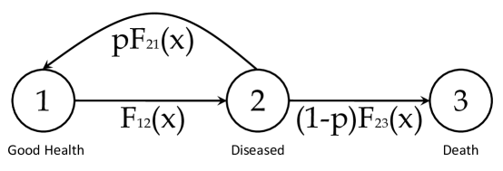
Figure 1: A SMP representation of the progress of a medical patient.

We begin the procedure with

$$\bm{P}=\left[\begin{array}[]{ccc}0&1&0\\ p&0&1-p\\ 0&0&1\\ \end{array}\right]\text{ and }\bm{N}=\left[\begin{array}[]{ccc}0&n_{12}&0\\ n_{21}&0&n_{23}\\ 0&0&n_{33}\\ \end{array}\right].$$

The expected first passage vector $\bm{M}_{3}$ to State 3 is then obtained as

$$\bm{M}_{3} = \left(\left[\begin{array}[]{ccc}1&0&0\\ 0&1&0\\ 0&0&1\\ \end{array}\right]-\left[\begin{array}[]{ccc}0&1&0\\ p&0&0\\ 0&0&0\\ \end{array}\right]\right)^{-1}\left(\left[\begin{array}[]{ccc}0&n_{12}&0\\ p\,n_{21}&0&(1-p)\,n_{23}\\ 0&0&n_{33}\\ \end{array}\right]\right)\left[\begin{array}[]{c}1\\ 1\\ 1\\ \end{array}\right]$$

$$= \frac{1}{1-p}\left[\begin{array}[]{ccc}1&1&0\\ p&1&0\\ 0&0&1-p\\ \end{array}\right]\left[\begin{array}[]{c}n_{12}\\ p\,n_{21}+(1-p)\,n_{23}\\ n_{33}\\ \end{array}\right]$$

$$= \frac{1}{1-p}\left[\begin{array}[]{c}n_{12}+p\,n_{21}+(1-p)\,n_{23}\\ p\,n_{12}+p\,n_{21}+(1-p)\,n_{23}\\ (1-p)\,n_{33}\\ \end{array}\right]$$

Looking closely at these values we can see they make sense. As $p$ gets small we can see $m_{13}\rightarrow n_{12}+n_{23}$ and $m_{23}\rightarrow n_{23}$. This simple example demonstrates the theory discussed earlier and how for even large systems find the first passage moments is only constrained by the computational burden of computing the inverse of $\bm{I}-\bm{P}+\bm{P}\bm{e}_{{}_{j}}\bm{e}_{{}_{j}}^{T}$.

If numbers are provided then numerical computer programs can handle these types of problems with ease. Now suppose we have

$$\bm{P}=\left[\begin{array}[]{ccc}0&1&0\\ 0.8&0&0.2\\ 0&0&1\\ \end{array}\right]\text{ and }\bm{N}=\left[\begin{array}[]{ccc}0&6&0\\ 0.7&0&1.1\\ 0&0&0\\ \end{array}\right].$$

We get the following result

$$\bm{M}_{3}=\left[\begin{array}[]{c}33.9\\ 27.9\\ 0\\ \end{array}\right].$$

The R-code for this example is included in the appendix. We feel the methods presented in this paper provide a comprehensive method to determine the first passage moments of a SMP.

7 Conclusion

In this paper we have devised an exact time-domain approach to derive the moments $m_{{}_{ij}}$ of first passage time distributions in reducible SMPs, given that the terminal state $j$ fulfills the conditions of universal accessibility. We note that the solution method presented here may be used to find the first passage moments of an irreducible SMP as well. This has the advantage of requiring the simultaneous solution of first passage moments to only single UA states $j$, rather than to all states, thereby reducing the computational load, particularly for large SMPs. We have also demonstrated the existence of consistent point estimators for the first passage moments of processes that may be modeled as SMPs.

8 Acknowledgements

The authors thank the editors and reviewers for providing feedback which improved the work.

9 Appendix

9.1 Properties of a Stochastic Matrix

The Perron-Frobenius theorem adapted to finite-dimensional irreducible and nonnegative matrices is very useful for characterizing the set of eigenvalues of such matrices. As we will see later, the theory may be (indirectly) extended to even reducible nonnegative matrices by leveraging their distinctive normal form. Let $\bm{A}\in\mathbb{R}_{{}_{+}}^{k\times k}$ for some positive integer $k$. We define the spectrum of $\bm{A}$, denoted $\sigma_{\bm{A}}$, to be the set of its eigenvalues. Its spectral radius, denoted $\rho(\bm{A})$, is given by

$$\rho(\bm{A})=\max\{|\lambda|:\lambda\in\sigma_{\bm{A}}\}\in\mathbb{R}_{{}_{+}},$$

which indicates the maximum radius of the disc that contains $\sigma_{\bm{A}}$ in the complex plane. Of particular interest is the case of a finite-dimensional stochastic matrix $\bm{A}$, which is a nonnegative square matrix such that $\bm{A}\,\bm{e}=\bm{e}$, where $\bm{e}$ is a column vector of ones. Perron-Frobenius theory, via Proposition 9.3 for the reducible case, implies that the spectral radius is likewise an eigenvalue of $\bm{A}$, denoted the Perron root of $\bm{A}$. Stochastic matrices comprise the boundary of the unit ball $\mathcal{A}=\{\bm{A}\in\mathbb{R}_{{}_{+}}^{k\times k}:||\bm{A}||_{\infty}\leq 1\}$ of finite-dimensional nonnegative matrices in the normed linear space induced by the infinity norm $||\cdot||_{\infty}$, which is given by the maximum absolute row sum of $\bm{A}=[a_{{}_{ij}}]$, or

$$||\bm{A}||_{\infty}=\max_{i}\sum_{j=1}^{k}{|a_{{}_{ij}}|}=\max(A\,\bm{e}).$$

As the next Proposition will show, we may classify certain elements of $\bm{A}\in\mathcal{A}$ with spectral radius $\rho(\bm{A})<1$ as substochastic, which is to say that $0<\min(\bm{A}\,\bm{e})<1$.

Proposition 9.1.

Suppose that $\bm{A}\in\mathcal{A}$. If $\rho(\bm{A})<1$, then $\bm{A}$ is substochastic.

Proof.

Clearly, since $\bm{A}\in\mathcal{A}$, it must be either stochastic or substochastic. Therefore the only thing that must be proved is that $\bm{A}$ is not stochastic. Assume $\bm{A}$ is stochastic; i.e. $\bm{A}\,\bm{e}=\bm{e}$. This implies $1$ is an eigenvalue, which contradicts $\rho(\bm{A})<1$. Therefore, $\bm{A}$ must be substochastic. ∎

For an irreducible nonnegative matrix $\bm{A}$, it is, in fact, sufficient for $\bm{A}$ to have a spectral radius that is strictly less than unity in order to be substochastic, as the next Proposition shows.

Proposition 9.2.

If $\bm{A}\in\mathbb{R}_{{}_{+}}^{k\times k}$ is an irreducible substochastic matrix, then $\rho(\bm{A})<1$.

Proof.

See Theorem 7 in [20]. ∎

The following Proposition relates the spectral radius of the sub-blocks of the matrix in normal form to that of the entire matrix.

Proposition 9.3.

Suppose $\bm{A}\in\mathbb{R}_{{}_{+}}^{k\times k}$ is a reducible matrix in normal form. Then $\rho(\bm{A})=\max_{\nu}\rho(\bm{A}_{\nu\nu})$ for $1\leq\nu\leq K$.

Proof.

See Lemma 1 in [18, pg. 303] with an additional induction argument to get the result or as argued in [9, pg.115]. ∎

9.2 Proof of Lemma 4.1

Proof.

We begin with the observation that, since $\bm{A}=[\bm{A}_{\nu\kappa}]=\bm{P}-\bm{P}\bm{e}_{{}_{j}}\bm{e}_{{}_{j}}^{T}$ is formed by setting each element of the $j^{\text{th}}$ column of $\bm{P}$ to 0, we essentially remove all directed arcs $(i,j)$ in the digraph $\mathcal{G}(\bm{P})$ for each $i\in V(\mathcal{G}(\bm{P}))$ in order to produce $\mathcal{G}(\bm{A})$. This means that $\mathcal{G}(\bm{A})$ cannot be strongly connected, and thus $\bm{A}$ must be reducible. We may therefore assume that $\bm{A}$ is in canonical form (1). Furthermore, because the $j^{\text{th}}$ column is zero, we will assume without loss of generality that the canonical form of $\bm{A}$ corresponds to the particular ordering of the states in $\mathcal{S}$ in which state $j$ is re-designated as state $1$. We impose the same permutation and partitioning on $\bm{P}=[\bm{P}_{\nu\kappa}]$ so that

$$\bm{A}_{\nu\kappa}=\begin{cases}\bm{P}_{\nu\kappa}&\text{if }(\nu,\kappa)\in\{1,\dots,K\}\times\{2,3,\ldots,K\},\\ \bm{0}&\text{if }(\nu,\kappa)\in\{1,\dots,K\}\times\{1\},\end{cases}$$ (12)

where, as in (1), $K$ is the dimension of $\bm{A}$. Notice that since $\bm{P}$ may be irreducible, the above does not necessarily imply that $\bm{P}$ can be put in canonical form, but rather is element-wise equivalent to $\bm{A}$, save for the first column, which, unlike that of $\bm{A}$, may contain positive entries. Stated succinctly, we have that

$$\bm{0}=\bm{A}_{\nu 1}\leq\bm{P}_{\nu 1},\qquad\nu=1,\dots,K.$$

Assume that $\left[\bm{I}-\bm{A}\right]$ is nonsingular, which directly implies that $1\notin\sigma_{\bm{A}}$; that is, $1$ is not an eigenvalue of $\bm{A}$. Since $\bm{P}$ is a row-stochastic matrix, and because of the equivalence given in (12), the Gerschgorin Circle Theorem (see [25, Eqn. 7.1.13]) indicates that the spectral radius $\delta=\rho(\bm{A})\leq 1$. Furthermore, the nonnegativity of $\bm{A}$ permits the use of Equation 8.3.1 of [25] to then assert that the Perron root $0\leq\delta\leq 1$ exists. However, since we have shown that $1\notin\sigma_{\bm{A}}$, it must then be the case that $\delta<1$. This implies by Proposition 9.3 that $\rho(\bm{A}_{\nu\nu})<1$ for all $\nu\in\{1,\dots,K\}$ and hence, by Proposition 9.2, each diagonal block $\bm{A}_{\nu\nu},\;\nu\in\{1,\dots,K\}$ must be substochastic.

We now consider the $\nu$th diagonal block in the canonical form of $\bm{A}$, where $\nu\in\{2,\dots,K\}$, and proceed to show that each state $i$ associated to the vertex set $V(\mathcal{G}(\bm{A}_{\nu\nu}))$ can access state $1$. Because $\bm{P}$ is a row-stochastic matrix and $A_{\nu\nu}$ is substochastic, either or both of the following may hold:

1. $\bm{P}_{\nu 1}\neq\bm{0}$, or

2. $\bm{A}_{\nu\kappa}\neq\bm{0}$ for some $\kappa>\nu$.

For 1), $\bm{P}_{\nu 1}\neq\bm{0}$ indicates the existence of states $i_{\nu}\in V(\mathcal{G}(\bm{A}_{\nu\nu}))$ (with $i_{\nu}=i$ possible, but not necessary) and $1\in V(\mathcal{G}(\bm{A}_{11}))$ for which there is a directed arc $(i_{\nu},1)$. Moreover, the irreducibility of $A_{\nu\nu}$ gives a directed path from $i$ to $i_{\nu}$. We thus obtain

$$i\rightarrow i_{\nu}\rightarrow 1.$$

In other words, there is a directed path from $i$ to 1.

If 2) holds, there exists a directed arc from some state $i_{\nu}\in V(\mathcal{G}(\bm{A}_{\nu\nu})$ (again, with the possibility that $i_{\nu}=i$) to a state $i_{\kappa}\in V(\mathcal{G}(\bm{A}_{\kappa\kappa}))$. From here, we are again confronted with choices 1) and 2). If 1) holds, then the previous argument gives us a directed path from $i_{\kappa}$ to 1. Since the irreducibility of $\bm{A}_{\nu\nu}$ implies the existence of a path from $i$ to $i_{\nu}$, we have the accessibility chain

$$i\rightarrow i_{\nu}\rightarrow i_{\kappa}\rightarrow 1,$$

and we are done. Otherwise, we proceed to the next diagonal block following $\bm{A}_{\kappa\kappa}$ and continue until we reach a state $i_{K}\in V(\mathcal{G}(\bm{A}_{KK}))$ in the last diagonal block $\bm{A}_{KK}$. The only choice here, due to the this block being substochastic, is 1); that is, $\bm{P}_{K1}\neq\bm{0}$, for which we have already demonstrated the existence of the connection $i_{K}\rightarrow 1$. Each of the preceding paths may then be combined to form a single directed path from an arbitrarily selected $i\in V(\mathcal{G}(\bm{A}_{\nu\nu}))$ to $1$ so that

$$i\rightarrow i_{\nu}\rightarrow i_{\kappa}\rightarrow\dots\rightarrow i_{K}\rightarrow 1.$$

Thus, state $1$ is UA.

For the reverse implication, we will assume that state $1$ is UA, and then proceed to show that $\left[\bm{I}-\bm{A}\right]$ is nonsingular. The reducibility of $\bm{A}$ allows us to assume that it possesses canonical form and, furthermore, that each submatrix on the diagonal of the canonical matrix corresponding to $\bm{A}$ is irreducible or zero. Consider an arbitrary nonzero, and hence irreducible, diagonal submatrix $\bm{A}_{\nu\nu}$ for some $\nu\in\{2,\dots,K\}$ (recall that $\bm{A}_{11}=\bm{0}$ by definition of $\bm{A}$). By the assumption that state $1$ is UA, there must be a directed path from each state in the vertex set $V(\mathcal{G}(\bm{A}_{\nu\nu}))$ to 1, which in turn implies that $\bm{A}_{\nu\nu}$ is substochastic. By Proposition 9.2, $\rho(\bm{A}_{\nu\nu})<1$. Using this fact, and the fact that the spectral radii of the zero submatrix blocks are 0, we may invoke Proposition 9.3, to state that $\rho(\bm{A})<1$. Hence, $\left[\bm{I}-\bm{A}\right]$ is nonsingular, which completes the proof. ∎

9.3 Comparing Equation (4) with Previous Results

To compare our main result, Equation (4), with Equation (5.12) of Hunter [11] we start by stating Equation (5.12) in our notation.

$$\bm{M}=\Big{[} \bm{G}\left(\bm{P}\circ\bm{N}\right)\bm{e}\bm{\pi}^{T}-\bm{E}\left(\bm{I}\circ\left(\bm{G}\left(\bm{P}\circ\bm{N}\right)\bm{e}\bm{\pi}^{T}\right)\right)+$$

$$\bm{\pi}^{T}\left(\bm{P}\circ\bm{N}\right)\bm{e}\left(\bm{I}-\bm{G}+\bm{E}\left(\bm{I}\circ\bm{G}\right)\right)\Big{]}\left[\bm{I}\circ\left(\bm{e}\bm{\pi}^{T}\right)\right]^{-1}.$$ (13)

In Equation (9.3), $\bm{G}$ represents any generalized inverse of $\bm{I}-\bm{P}$ and $\bm{\pi}$ is the stationary distribution of the process. However, in our methodology we require a specific generalized inverse of $\bm{I}-\bm{P}$, which is

$$\left[\bm{I}-\bm{P}+\bm{P}\bm{e}_{{}_{j}}\bm{e}_{{}_{j}}^{T}\right]^{-1}.$$ (14)

In our methodology we only find the first passage moments from all states to state $j$ (assuming $j$ is UA). Using Equation (9.3) one must assume an irreducible process.

It can be shown if $\bm{G}$ is a generalized inverse of $\bm{I}-\bm{P}$ in the form of Equation (14), the $j^{\text{th}}$ column of the matrix

$$-\bm{E}\left(\bm{I}\circ\left(\bm{G}\left(\bm{P}\circ\bm{N}\right)\bm{e}\bm{\pi}^{T}\right)\right)+\bm{\pi}^{T}\left(\bm{P}\circ\bm{N}\right)\bm{e}\left(\bm{I}-\bm{G}+\bm{E}\left(\bm{I}\circ\bm{G}\right)\right)$$

is identically zero. Removing those terms, substituting Equation (14) for $\bm{G}$, and eliminating all but the $j^{\text{th}}$ column of Equation (9.3) yields

$$\bm{M}_{j} =\left(\left[\left[\bm{I}-\bm{P}+\bm{P}\bm{e}_{{}_{j}}\bm{e}_{{}_{j}}^{T}\right]^{-1}\left(\bm{P}\circ\bm{N}\right)\bm{e}\bm{\pi}^{T}\right]\left[\bm{I}\circ\left(\bm{e}\bm{\pi}^{T}\right)\right]^{-1}\right)_{j}$$

$$=\left[\bm{I}-\bm{P}+\bm{P}\bm{e}_{{}_{j}}\bm{e}_{{}_{j}}^{T}\right]^{-1}\left(\bm{P}\circ\bm{N}\right)\bm{e}.$$

This last equation is identical to our Equation (4). This demonstrates how our methodology ties into the previous literature, which assumes an irreducible process.

9.4 R-Code for Example

P <- matrix(c(0,1,0,.8,0,.2,0,0,1),ncol=3,nrow=3,byrow=T)
N <- matrix(c(0,6,0,.7,0,1.1,0,0,0),ncol=3,nrow=3,byrow=T)
I <- diag(3)
e3 <- c(0,0,1)
e <- matrix(1,ncol=1,nrow=3)
m3 <- solve(I-P+P%*%e3%*%t(e3))%*%(P*N)%*%e
m3

Richard L. Warr
Brigham Young University
223 TMCB
Provo, UT 84602
E-mail: richard.L.warr@gmail.com

James D. Cordeiro
University of Dayton
300 College Park
Dayton, OH 45469
E-mail: jcordeiro1@udayton.edu

References

- [1] V. Barbu, M. Boussemart, and N. Limnios, Discrete-time semi-Markov model for reliability and survival analysis, Commun Stat-Theor M 33 (2004), no. 11, 2833=962868.
- [2] Vlad Stefan Barbu and Nikolaos Liminios, Semi-Markov chains and hidden semi-Markov models toward = applications: Their use in reliability and DNA analysis, Springer, New York, 2008.
- [3] R.E. Barlow and F. Proschan, Mathematical theory of reliability, John Wiley & Sons, London and New York, 1965.
- [4] Shelby Brumelle and Darius Walczak, Dynamic airline revenue management with multiple semi-Markov demand, Operations Research 51 (2003), no. 1, 137–148.
- [5] Ronald W. Butler and Aparna V. Huzurbazar, Stochastic network models for survival analysis, J. Amer. Statist. Assoc. 92 (1997), 246–257. MR MR1436113 (98e:62140)
- [6] George Casella and Roger L. Berger, Statistical inference, second ed., Duxbury, Pacific Grove, CA., 2002.
- [7] E. Çınlar, Introduction to stochastic processes, Prentice-Hall, Englewood Cliffs, NJ, 1975.
- [8] Guglielmo D’Amico, Jacques Janssen, and Raimondo Manca, Homogeneous semi-Markov reliability models for credit risk management, Decisions in Economics and Finance 28 (2006), 79–93.
- [9] Miroslav Fiedler, Special matrices and their applications in numerical mathematics, 2nd ed., Dover Publications, New York, 2008.
- [10] Jeffrey J. Hunter, On the moments of Markov renewal processes, Advances in Applied Probability 1 (1969), no. 2, 188–210.
- [11] , Generalized inverses and their application to applied probability problems, Linear Algebra and its Applications 45 (1982), 157–198.
- [12] , Simple procedures for finding mean first passage times in Markov chains, Asia-Pacific Journal of Operational Research 24 (2007), no. 6, 813–829.
- [13] , Accurate calculations of stationary distributions and mean first passage times in Markov renewal processes and markov chains, Special Matrices 4 (2016), no. 1, 151–175.
- [14] , The computation of the mean first passage times for Markov chains, Linear Algebra and its Applications 549 (2018), 100 – 122.
- [15] Jacques Janssen and Raimondo Manca, Semi-Markov risk models for finance, insurance, and reliability, Springer, New York, 2007.
- [16] J.G. Kemény and J.L. Snell, Finite Markov chains, University series in undergraduate mathematics, Van Nostrand, 1960.
- [17] Jeffrey P. Kharoufeh, Christopher J. Solo, and M.Y. Ulukus, Semi-Markov models for degradation-based reliability, IIE Transactions 42 (2010), no. 8, 599–612.
- [18] David Kincaid and Ward Cheney, Numerical analysis: mathematics of scientific computing, 3rd ed., vol. 2, American Mathematical Society, Providence, 2002.
- [19] Leonard Kleinrock, Queueing systems volume I: Theory, John Wiley & Sons, New York, 1975.
- [20] V.V. Kolpakov, Matrix seminorms and related inequalities, Journal of Mathematical Sciences 23 (1983), no. 1, 2094–2106.
- [21] Steven R Lerman, The use of disaggregate choice models in semi-Markov process models of trip chaining behavior, Transportation Science 13 (1979), no. 4, 273–291.
- [22] P. Levy, Processus semi-Markoviens, Proc. Intern. Congr. Math. 3 (1954), 416–426, Amsterdam, The Netherlands.
- [23] , Systems semi-Markoviens ayant au plus une inifinite denombrable d’etats possibles, Proc. Intern. Congr. Math. 2 (1954), 294–295, Amsterdam, The Netherlands.
- [24] N. Limnios and G. Oprişan, Semi-Markov processes and reliability, Birkhäuser, Boston, 2001.
- [25] Carl D. Meyer, Matrix analysis and applied linear algebra, Society for Industrial Mathematics, Philadelphia, 2000.
- [26] M.F. Neuts, Structured stochastic matrices of type and their applications, Probability: Pure and Applied, Marcel Dekker, Inc., New York and Basel, 1989.
- [27] Ronald Pyke, Markov renewal processes: Definitions and preliminary properties, The Annals of Mathematical Statistics 32 (1961), no. 4, 1231–1242.
- [28] , Markov renewal processes with finitely many states, The Annals of Mathematical Statistics 32 (1961), no. 4, 1243–1259.
- [29] Sheldon M. Ross, Applied probability models with optimization applications, Holden-Day, San Francisco, 1970.
- [30] Jia-Yu Shao, Products of irreducible matrices, Linear Algebra and Its Applications 68 (1985), 131–143.
- [31] W. L. Smith, Regenerative stochastic processes, Proc. Roy. Soc (GB), series A, 232 (1955), 6–31, Amsterdam, The Netherlands.
- [32] Arun Veeramany and Mahesh D Pandey, Reliability analysis of nuclear piping system using semi-markov process model, Annals of Nuclear Energy 38 (2011), no. 5, 1133–1139.
- [33] George H Weiss and Marvin Zelen, A semi-Markov model for clinical trials, Journal of Applied Probability 2 (1965), no. 2, 269–285.
- [34] David D. Yao, First-passage-time moments of Markov processes, Journal of Applied Probability 22 (1985), no. 4, 939–945.
- [35] H.L.S. Younes and R.G. Simmons, Solving generalized semi-Markov decision processes using continuous phase-type distributions, Proceeding of the National Conference on Artificial Intelligence, 2004, pp. 742–747.
- [36] Xuan Zhang and Zhenting Hou, The first-passage times of phase semi-Markov processes, Statistics & Probability Letters 82 (2012), no. 1, 40 – 48.