$W^{2,1}$ estimate for singular solutions to the Monge-Ampère equation

Abstract.

We prove an interior $W^{2,1}$ estimate for singular solutions to the Monge-Ampère equation, and construct an example to show our results are optimal.

Mathematics Subject Classification 35J96, 35B65.

1. Introduction

Interior $W^{2,p}$ estimates for the Monge-Ampère equation

$$\det D^{2}u=f\quad\text{ in }\Omega,\quad\quad u|_{\partial\Omega}=0$$

were first obtained by Caffarelli assuming that $f$ has small oscillation depending on $p$ (see [C2]).

In the case that we only have $\lambda\leq f\leq\Lambda,$ De Philippis, Figalli and Savin recently obtained interior $W^{2,1+\epsilon}$ estimates for some $\epsilon$ depending only on $n,\Lambda$ and $\Lambda$ (see [DF],[DFS]). This result is optimal in light of counterexamples due to Wang ([W]) obtained by seeking solutions with the homogeneity

$$u(x,y)=\frac{1}{\lambda^{2+\alpha}}u(\lambda x,\lambda^{1+\alpha}y).$$

These can be viewed as estimates for strictly convex solutions to the Monge-Ampère equation. Indeed, at a point $x$ where $u$ is strictly convex we can find a tangent plane that touches only at $x$ and lift it a little to carve out a set where $u$ has linear boundary data.

In [M] we show that solutions to $\lambda\leq\det D^{2}u\leq\Lambda$ are strictly convex away from a singular set of Hausdorff $n-1$ dimensional measure zero, and as a consequence we prove $W^{2,1}$ regularity for singular solutions. We also construct for any $\epsilon$ a singular solution to $\det D^{2}u=1$ in $B_{1}\subset\mathbb{R}^{n}$ ($n\geq 3$) with a singular set of Hausdorff dimension at least $n-1-\epsilon$ which is not in $W^{2,1+\epsilon}$. However, as $\epsilon\rightarrow 0$ these examples become arbitrarily large. In this paper we give a more precise, quantitative version of the work done in [M] and improve the examples. Our main theorem is:

Theorem 1.1.

Assume that

$$\lambda\leq\det D^{2}u\leq\Lambda\quad\text{ in }B_{1}\subset\mathbb{R}^{n},\quad\quad\|u\|_{L^{\infty}(B_{1})}<K.$$

Then for some $\epsilon(n)$ and $C(n,\lambda,\Lambda,K)$ we have $\Delta u\in L\log^{\epsilon}L$ and

$$\int_{B_{1/2}}\Delta u\left(\log(1+\Delta u)\right)^{\epsilon}\,dx\leq C.$$

We also construct an example with a singular set of Hausdorff dimension exactly $n-1$ and second derivatives not in $L\log^{M}L$ for $M$ large, showing that the main theorem is in a sense optimal and that we cannot improve our estimate on the Hausdorff dimension to $n-1-\epsilon$ for any $\epsilon$. Since solutions in two dimensions are strictly convex, this result is interesting for $n\geq 3$.

The paper is organized as follows. In section $2$ we present some preliminaries on the geometry of sections. In section $3$ we state our key proposition and use it to prove Theorem 1.1. In section $4$ we prove the key proposition, which is a quantitative version of work done in [M] obtained by closely examining the geometry of maximal sections. Finally, in sections $5$ and $6$ we construct an example with a singular set of Hausdorff dimension $n-1$ and show that it gives optimality of Theorem 1.1.

2. Preliminaries

Let $u:\Omega\subset\mathbb{R}^{n}\rightarrow\mathbb{R}$ be a convex function. Then $u$ has an associated Borel measure $Mu$, called the Monge-Ampère measure, defined by

$$Mu(A)=|\nabla u(A)|$$

where $|\nabla u(A)|$ represents the Lebesgue measure of the image of the subgradients of $u$ in $A$ (see [Gut]). We say that $u$ solves $\det D^{2}u=f$ in the Alexandrov sense if

$$Mu=f\,dx.$$

We define a section of $u$ by

$$S_{h}(x)=\{y\in\Omega:u(y)<u(x)+\nabla u(x)\cdot(y-x)+h\}$$

for some subgradient $\nabla u(x)$ at $x$. Finally, we define $D_{n,\lambda,\Lambda,K}$ to be the collection of convex functions satisfying

$$\lambda\leq\det D^{2}u\leq\Lambda\quad\text{ in }B_{1}\subset\mathbb{R}^{n},\quad\quad\|u\|_{L^{\infty}(B_{1})}\leq K$$

in the Alexandrov sense and we say that a constant depending only on $n,\lambda,\Lambda$ and $K$ is a universal constant. In this section we recall some geometric observations about sections of solutions in $D_{n,\lambda,\Lambda,K}$.

Lemma 2.1.

(John’s Lemma). If $S\subset\mathbb{R}^{n}$ is a bounded convex set with nonempty interior, and $0$ is the center of mass of $S$, then there exists an ellipsoid $E$ and a dimensional constant $C(n)$ such that

$$E\subset S\subset C(n)E.$$

We call $E$ the John ellipsoid of $S$. There is some linear transformation $A$ such that $A(B_{1})=E$, and we say that $A$ normalizes $S$.

In the following two lemmas we present an important observation on the volume growth of sections that are not compactly contained and relate the volume of compactly contained sections to the Monge-Ampère mass of these sections. Short proofs can be found in [M].

Lemma 2.2.

Assume that $\det D^{2}u\geq\lambda$ in $\Omega\subset\mathbb{R}^{n}$. Then if $S_{h}(x)$ is any section of $u$, we have

$$|S_{h}(x)|\leq Ch^{n/2}$$

for some constant $C$ depending only on $\lambda$ and $n$.

The proof is just a barrier by above in the John ellipsoid for $S_{h}(x)$.

Lemma 2.3.

Let $v$ be any convex function on $\Omega\subset\mathbb{R}^{n}$ with $v|_{\partial\Omega}=0$. Then

$$Mv(\Omega)\,|\Omega|\geq c(n)|\min_{\Omega}v|^{n}.$$

The proof is by comparing to the Monge-Ampère mass of the function whose graph is the cone generated by the minimum point of $v$ and $\partial\Omega$.

Next, we recall the following geometric observation of Caffarelli for solutions to the Monge-Ampère equation with bounded right hand side (see [C1]). It says that compactly contained sections $S_{h}(x)$ are balanced around $x$.

Lemma 2.4.

Assume that $\lambda\leq\det D^{2}u\leq\Lambda$ in $\Omega\subset\mathbb{R}^{n}$. Then there exist $c,C(n,\lambda,\Lambda)$ such that for all $S_{h}(x)\subset\subset\Omega$, there is an ellipsoid $E$ centered at $0$ of volume $h^{n/2}$ with

$$cE\subset S_{h}(x)-x\subset CE.$$

Finally, we give the following engulfing and covering properties of compactly contained sections (see [CG] and [DFS]). In the following $\alpha S_{h}(x)$ will denote the $\alpha$ dilation of $S_{h}(x)$ around $x$.

Lemma 2.5.

Assume that $\lambda\leq\det D^{2}u\leq\Lambda$ in $\Omega$. Then there exists $\delta>0$ universal such that:

1. If $S_{h}(x)\subset\subset\Omega$ then

   $$S_{\delta h}(x)\subset\frac{1}{2}S_{h}(x).$$

2. Suppose that for some compact $D\subset\Omega$, we can associate to each $x\in D$ some $S_{h}(x)\subset\subset\Omega$. Then we can find a finite subcollection $\{S_{h_{i}}(x_{i})\}_{i=1}^{M}$ such that $S_{\delta h_{i}}(x_{i})$ are disjoint and

   $$D\subset\cup_{i=1}^{M}S_{h_{i}}(x_{i}).$$

3. Statement of Key Proposition and Proof of Theorem 1.1

In this section we state the key proposition and use it to prove our main theorem. In [M] we show that the Monge-Ampere mass of $u+\frac{1}{2}|x|^{2}$ in small balls around singular points is large compared to the mass of $\Delta u$. The proposition is a more precise, quantitative version of this statement for long, thin sections. Let $\bar{h}(x)\geq 0$ be the largest $h$ such that $S_{h}(x)\subset\subset B_{1}$. We say that $S_{\bar{h}(x)}(x)$ is the maximal section at $x$. If $\bar{h}(x)=0$ then $x$ is a singular point.

Proposition 3.1.

If $u\in D_{n,\lambda,\Lambda,K}$, $v=u+\frac{1}{2}|x|^{2}$, $x\in B_{1/2}$ and $h>\bar{h}(x)$ then there exist $\eta(n)$ and $c$ universal such that for some $r$ with

$$|\log r|>c|\log h|^{1/2},$$

we have

$$Mv(B_{r}(x))>cr^{n-1}|\log r|^{\eta}.$$

Remark 3.2.

Let $\Sigma$ denote the singular set of $u$, where $\bar{h}=0$. It follows from proposition 3.1 and a covering argument that

$$\inf_{\delta>0}\left\{\sum_{i=1}^{\infty}r_{i}^{n-1}|\log r_{i}|^{\eta}:\{B_{r_{i}}(x_{i})\}_{i=1}^{\infty}\text{ cover }\Sigma,r_{i}<\delta\right\}=0$$

for some small $\eta(n)$, giving a quantitative version of the main theorem in [M] for solutions to $\lambda\leq\det D^{2}u\leq\Lambda$.

We will give a proof of Proposition 3.1 in the next section by closely examining the geometric properties of maximal sections.

The idea of the proof of Theorem 1.1 is to apply Proposition 3.1 in the thin maximal sections, and then apply the $W^{2,1+\epsilon}$ estimate of [DFS] in the larger sections to show the following decay of the integral of $\Delta u$ over its level sets:

(1) $$\int_{\{\Delta u>t\}}\Delta u\,dx\leq\frac{C}{|\log t|^{\epsilon}},$$

for some $\epsilon(n)$. Assuming this is true, theorem 1.1 follows easily by Fubini:

$$\int_{B_{1/2}}\Delta u(\log(1+\Delta u))^{\epsilon/2}\,dx \leq C\int_{B_{1/2}}\Delta u\int_{1}^{1+\Delta u}\frac{1}{t(\log t)^{1-\epsilon/2}}\,dt\,dx$$

$$\leq C+C\int_{2}^{\infty}\frac{1}{t(\log t)^{1-\epsilon/2}}\int_{\{\Delta u>t\}}\Delta u\,dx\,dt$$

$$\leq C+C\int_{2}^{\infty}\frac{1}{t(\log t)^{1+\epsilon/2}}\,dt$$

$$\leq C(\epsilon).$$

To prove (1), We first recall the following theorem of De Philippis, Figalli and Savin:

Theorem 3.3.

Assume that

$$\lambda\leq\det D^{2}u\leq\Lambda\quad\text{ in }S_{H}(0),\quad\quad u|_{\partial S_{H}(0)}=0$$

and $B_{1}$ is the John ellipsoid for $S_{H}(0)$. Then there exist $C,\epsilon$ depending only on $\lambda,\Lambda$ and $n$ such that

$$\int_{S_{H/2}(0)\cap\{\Delta u>t\}}\Delta u\,dx<Ct^{-\epsilon}.$$

We will use the rescaled version of this theorem in the larger maximal sections.

Lemma 3.4.

If $u\in D_{n,\lambda,\Lambda,K}$ with $x\in B_{1/2}$ and $S_{h}(x)\subset\subset B_{1}$, then for $C$ universal and $\epsilon(n,\lambda,\Lambda)$ we have

$$\int_{S_{h/2}(x)\cap\{\Delta u>t\}}\Delta u\,dx<Ch^{n/2-1-\epsilon}t^{-\epsilon}.$$

Proof.

By subtracting a linear function and translating assume that $x=0$ and $u|_{\partial S_{h}(0)}=0$. Let

$$u(x)=(\det A)^{2/n}\tilde{u}(A^{-1}x)$$

where $A$ normalizes $S_{h}(x)$ and $\tilde{u}$ has height $H$. Then

$$D^{2}u(x)=C|S_{h}(0)|^{2/n}(A^{-1})D^{2}\tilde{u}(A^{-1}x)(A^{-1})^{T}.$$

Applying the estimate on $|S_{h}(0)|$ from Lemma 2.4 and letting $d$ denote the length of the smallest axis for the John ellipsoid of $S_{h}(0)$, it follows that

$$\Delta u(x)\leq C\left(\frac{h}{d^{2}}\right)\Delta\tilde{u}(A^{-1}x).$$

Using change of variables and Theorem 3.3 we obtain that

$$\int_{S_{h/2}(0)\cap\{\Delta u>t\}}\Delta u\,dx \leq C(\det A)\left(\frac{h}{d^{2}}\right)\int_{S_{H/2}(0)\cap\{\Delta\tilde{u}>c\frac{d^{2}}{h}t\}}\Delta\tilde{u}(y)\,dy$$

$$\leq C(\det A)\left(\frac{h}{d^{2}}\right)^{1+\epsilon}t^{-\epsilon}.$$

Since $\det A=h^{n/2}$ up to a universal constants and $d>ch$ since $u$ is locally Lipschitz, the conclusion follows. ∎

Let $F_{\gamma}=\{x\in B_{1/2}:\frac{\gamma}{2}\leq\bar{h}(x)<\gamma\}.$

Lemma 3.5.

Let $u\in D_{n,\lambda,\Lambda,K}$. Then there is some $C$ universal and $\epsilon(n,\lambda,\Lambda)$ such that

$$\int_{F_{\gamma}\cap\{\Delta u>t\}}\Delta u\,dx<C\gamma^{-\epsilon}t^{-\epsilon}$$

Proof.

By Lemma 2.5 we can take a cover of $F_{\gamma}$ by sections $\{S_{\bar{h_{i}}(x_{i})/2}(x_{i})\}_{i=1}^{M_{\gamma}}$ with $x_{i}\in F_{\gamma}$ and $S_{\delta\bar{h_{i}}(x_{i})}(x_{i})$ disjoint for some universal $\delta$. Then

$$\int_{F_{\gamma}\cap\{\Delta u>t\}}\Delta u\,dx\leq CM_{\gamma}\gamma^{n/2-1-\epsilon}t^{-\epsilon}$$

by Lemma 3.4. We need to estimate the number of sections $M_{\gamma}$ in our Vitali cover of $F_{\gamma}$.

Take $x\in F_{\gamma}$ and consider $S_{\bar{h}(x)}(x)$, which touches $\partial B_{1}$. By translation and subtracting a linear function assume that $x=0$ and $u|_{\partial S_{\delta^{2}\bar{h}(0)}(0)}=0$. By rotating and applying Lemma 2.4 assume that $S_{\delta^{2}\bar{h}(0)}(0)$ contains the line segment from $-ce_{n}$ to $ce_{n}$, with $c$ universal.

Let $w_{t}$ be the restriction of $u$ to $\{x_{n}=t\}$ and let

$$S^{w_{t}}=S_{\delta^{2}\bar{h}(0)}(0)\cap\{x_{n}=t\}$$

be the slice of $S_{\delta^{2}\bar{h}(0)}(0)$ at $x_{n}=t$. Since $|S_{\delta^{2}\bar{h}(0)}(0)|\leq C\gamma^{n/2}$ and this section has length $2c$ in the $e_{n}$ direction, it follows from convexity that

$$|S^{w_{t}}|_{\mathcal{H}^{n-1}}\leq C\gamma^{n/2}.$$

By convexity, $u(te_{n})<-\delta^{2}\bar{h}(0)/2$ for $-c/2\leq t\leq c/2$. Applying Lemma 2.3, we conclude that for $t\in[-c/2,c/2]$,

$$Mw_{t}(S^{w_{t}})>c\gamma^{n/2-1}.$$

Let $r$ be the distance between $\partial S_{\delta^{2}\bar{h}(0)}(0)$ and $\partial(2S_{\delta^{2}\bar{h}(0)}(0))$. Divide $2S_{\delta^{2}\bar{h}(0)}(0)$ into the slices

$$S_{k}=2S_{\delta^{2}\bar{h}(0)}(0)\cap\{kr<x_{n}<(k+1)r\}$$

for $k=-\frac{c}{2r}$ to $\frac{c}{2r}$. Let $v=u+\frac{1}{2}|x|^{2}$. Then $\nabla v(S_{k})$ contains a ball of radius $r/2$ around each point in $\nabla v(S^{w_{(k+1/2)r}})$ (see Figure 1), so

$$Mv(S_{k})\geq crMv(S^{w_{(k+1/2)r}})\geq cr\gamma^{n/2-1}.$$

Summing from $k=-\frac{c}{2r}$ to $\frac{c}{2r}$ we obtain that

$$|\nabla v(2S_{\delta^{2}\bar{h}(0)}(0))|\geq c\gamma^{n/2-1}.$$

Using that $2S_{\delta^{2}\bar{h}_{i}}(x_{i})\subset S_{\delta\bar{h}_{i}}(x_{i})$ are disjoint and summing over $i$ we obtain that

$$M_{\gamma}\gamma^{n/2-1}<C$$

and the conclusion follows.

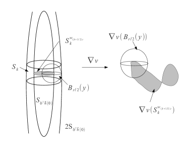
Figure 1. $\nabla v(S_{k})$ contains an $r/2$-neighborhood of the surface $\nabla v(S^{w_{(k+1/2)r}})$, which projects in the $x_{n}$ direction to a set of $\mathcal{H}^{n-1}$ measure at least $c\gamma^{n/2-1}$.

∎

Proof of Theorem 1.1.

We first consider the set where $\bar{h}(x)\leq\frac{1}{t^{1/2}}$. At any point in this set, by Proposition 3.1, we can find some $r>0$ such that $|\log r|>c|\log t|^{1/2}$ and

$$Mv(B_{r}(x))>cr^{n-1}(\log t)^{\eta/2}.$$

We conclude that

$$\int_{B_{r}(x)}\Delta u\,dx\leq Cr^{n-1}\leq\frac{C}{(\log t)^{\eta/2}}Mv(B_{r}(x)).$$

Covering $\{\Delta u>t\}\cap\{\bar{h}(x)\leq\frac{1}{t^{1/2}}\}$ with these balls and taking a Vitali subcover $\{B_{r_{i}}(x_{i})\}$, we obtain that

$$\int_{\{\Delta u>t\}\cap\{\bar{h}(x)<\frac{1}{t^{1/2}}\}}\Delta u\,dx\leq\frac{C}{(\log t)^{\eta/2}}\sum_{i}Mv(B_{r_{i}}(x_{i}))\leq\frac{C}{(\log t)^{\eta/2}},$$

giving the desired bound over the “near-singular” points.

We now study the integral of $\Delta u$ over the remaining subset of $\{\Delta u>t\}$. Take $k_{0}$ so that

$$2^{k_{0}-1}\leq t^{1/2}<2^{k_{0}}.$$

Applying Lemma 3.5 we obtain that

$$\int_{\{\Delta u>t\}\cap\{\bar{h}(x)>\frac{1}{t^{1/2}}\}}\Delta u\,dx \leq\sum_{i=0}^{k_{0}}\int_{\{\Delta u>t\}\cap F_{2^{-i}}}\Delta u\,dx$$

$$\leq Ct^{-\epsilon}\sum_{i=1}^{k_{0}}2^{\epsilon i}$$

$$\leq Ct^{-\epsilon/2},$$

giving the desired bound. ∎

4. Quantitative Behavior of Maximal Sections

In this section we closely examine the geometric properties of maximal sections of solutions in $D_{n,\lambda,\Lambda,K}$ to prove Proposition 3.1.

Let $u\in D_{n,\lambda,\Lambda,K}$ and fix $x\in B_{1/2}$. Then for any $h>\bar{h}(x)$, $S_{h}(x)$ is not compactly contained in $\partial B_{1}$. If $\bar{h}(x)>0$, then by Lemma 2.4, $S_{\bar{h}(x)}(x)$ contains an ellipsoid $E$ centered at $x$ with a long axis of universal length $2c$.

If $\bar{h}(x)=0$ and $L$ is the tangent to $u$ at $x$ then it is a consequence of lemma 2.4 (see [C1]) that $\{u=L\}$ has no extremal points, and in particular for any $h>0$ we know $S_{h}(x)$ contains a line segment (independent of $h$) exiting $\partial B_{1}$ at both ends.

By translating and subtracting a linear function assume that $x=0$ and $\nabla u(0)=0$. By rotating assume that $S_{h}(0)$ contains the line segment from $-ce_{n}$ to $ce_{n}$ for all $h>\bar{h}(0)$. For the rest of the section denote $\bar{h}(0)$ by just $\bar{h}$.

Let $w$ be the restriction of $u$ to $\{x_{n}=0\}$ with sections $S_{h}^{w}$. Since $|S_{h}(0)|<Ch^{n/2}$ for all $h$ and $S_{\bar{h}}(0)$ contains a line segment of universal length in the $e_{n}$ direction, we have

$$|S_{h}^{w}(0)|_{\mathcal{H}^{n-1}}<Ch^{n/2}$$

for $h\geq\bar{h}$. In the following analysis we need to focus on those sections of $w$ with the same volume bound. The following property is sufficient:

Property $F$: We say $S_{h}^{w}(y)$ satisfies property $F$ if

$$w(y)+\nabla w(y)\cdot(-y)+h\geq\bar{h}.$$

(See Figure 2).

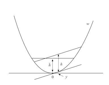
Figure 2. $S_{h}^{w}(y)$ satisfies property $F$ if the tangent plane at $y$, lifted by $h$, lies above $\bar{h}$ at $0$.

Lemma 4.1.

If $S_{h}^{w}(y)$ satisfies property $F$ then

$$|S_{h}^{w}(y)|<Ch^{n/2}.$$

Proof.

The plane $u(y)+\nabla u(y)\cdot(z-y)+h$ is greater than $\bar{h}$ along $z=te_{n}$ for either $t>0$ or $t<0$. Since $u<\bar{h}$ on the segment from $-ce_{n}$ to $ce_{n}$, it follows that $S_{h}(y)$ contains the line segment from $0$ to $ce_{n}$ or $-ce_{n}$. Since $|S_{h}(y)|<Ch^{n/2}$ the conclusion follows. ∎

The first key lemma says that $w$ grows logarithmically faster than quadratic in at least two directions at a level comparable to $\bar{h}$. Let

$$d_{1}^{y}(h)\geq d_{2}^{y}(h)\geq...\geq d_{n-1}^{y}(h)$$

denote the axis lengths of the John ellisoid for $S_{h}^{w}(y)$.

Lemma 4.2.

For any $h>\bar{h}$ there exist $\epsilon(n)$, $C_{0}$ universal, $h_{0}<e^{-|\log h|^{1/2}}$ and $y$ such that $S_{h_{0}}^{w}(y)$ satisfies property $F$ and

$$d_{n-2}^{y}(h_{0})<C_{0}h_{0}^{1/2}|\log h_{0}|^{-\epsilon}.$$

The next lemma says that if $w$ grows logarithmically faster than quadratic in at least two directions up to height $h$ then the Monge-Ampère mass of $u+\frac{1}{2}|x|^{2}$ is logarithmically larger than the mass of $\Delta u$ in a ball with radius comparable to $h^{1/2}$.

Lemma 4.3.

Fix $\epsilon>0$ and assume that for some $h>0$, $S_{h}^{w}(y)$ satisfies property $F$. Then there exist $\eta_{1},\eta_{2}(n,\epsilon)$ and $C$ depending on universal constants and $\epsilon$ such that if

$$d_{n-2}^{y}(h)<h^{1/2}|\log h|^{-\epsilon}$$

then for some $r<Ch^{1/2}|\log h|^{-\eta_{1}}$ we have

$$M\left(u+\frac{1}{2}|x|^{2}\right)(B_{r}(0))>C^{-1}r^{n-1}|\log r|^{\eta_{2}}.$$

These lemmas combine to give the key proposition:

Proof of Proposision 3.1:.

By Lemma 4.2, there is some $S_{h}(y)$ satisfying property $F$ with

$$d_{n-2}^{y}(h)<C_{0}h^{1/2}|\log h|^{-\epsilon},$$

with $\epsilon(n)$, $C_{0}$ universal and $h<e^{-|\log(\delta+\bar{h}(x))|^{1/2}}$ for any $\delta$. The conclusion follows from Lemma 4.3. ∎

We now turn to the proofs of Lemmas 4.2 and 4.3.

Proof of Lemma 4.2.

Assume by way of contradiction that for all $h<h_{0}$ and $S_{h}^{w}(y)$ satisfying property $F$ we have

$$d_{n-2}^{y}(h)>C_{0}h^{1/2}|\log h|^{-\epsilon},$$

for $h_{0}$ depending on $\bar{h}$ and $C_{0},\epsilon$ we will choose later. We divide the proof into two steps.

Step 1: Define the breadth $b(h)$ as the minimum distance between two parallel tangent hyperplanes to $\partial S_{h}^{w}(0)$. We show that for $\bar{h}|\log\bar{h}|<h<h_{0}$ we have

$$b(h/2)>\left(\frac{1}{2}+\frac{C_{1}}{|\log h|}\right)b(h)$$

for some $C_{1}$ large depending on $C_{0}$. Let $x_{0}$ be the center of mass of $S_{h}^{w}(0)$ and rotate so that the John ellipsoid for $S_{h}^{w}(0)$ is $A(B_{1})+x_{0}$, where

$$A=\text{diag}(d_{1}^{0}(h),...,d_{n-1}^{0}(h)).$$

Let $P_{1},P_{2}$ be the tangent hyperplanes to $\partial S_{h/2}^{w}(0)$ a distance $b(h/2)$ apart. Let $x_{1},x_{2}$ be points where $P_{1}$ and $P_{2}$ become tangent to $\partial S_{h}^{w}(0)$ when we slide them out. Assume that the distance between $0$ and the plane tangent at $x_{1}$ is larger than that between $0$ and the plane tangent at $x_{2}$. (See Figure 3).

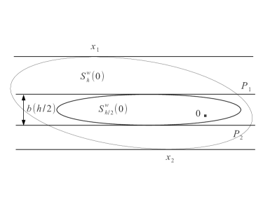
Figure 3.

Let $\tilde{x}_{1}$ be the image of $x_{1}$ under $A^{-1}$ and let

$$\tilde{w}(x)=(\det A)^{-2/n}w(Ax).$$

Observe that $\tilde{w}$ is the restriction of $\tilde{u}(x)=(\det A)^{-2/n}u(Ax^{\prime},x_{n})$ which solves $\lambda\leq\det D^{2}u\leq\Lambda$, so that sections $S_{h}^{\tilde{w}}$ of $\tilde{w}$ satisfying property $F$ with $\bar{h}$ replaced by $(\det A)^{-2/n}\bar{h}$ have volume bounded above by $Ch^{n/2}$. Furthermore, since the distance between $0$ and the plane tangent at $x_{1}$ was larger and the images of the tangent planes under $A^{-1}$ are separated by distance at least $2$, we have $|\tilde{x}_{1}|\geq 1$.

By convexity we can find $\tilde{y}$ on the line segment connecting $0$ to $\tilde{x}_{1}$ such that

$$\nabla\tilde{w}(\tilde{y})\cdot\frac{\tilde{x}_{1}}{|\tilde{x}_{1}|}=\frac{H}{|\tilde{x}_{1}|},$$

where $H=\det A^{-2/n}h$ is the height of $\tilde{w}$. Let $\tilde{h}$ be the smallest $t$ such that $0\in S_{t}^{\tilde{w}}(\tilde{y})$. We aim to bound $\tilde{h}$ below, which heuristically rules out cone-like behavior in the $\tilde{x}_{1}$ direction. Let

$$h^{*}=\tilde{h}+(\det A)^{-2/n}\bar{h}.$$

We have chosen $h^{*}$ so that $S_{h^{*}}^{\tilde{w}}(\tilde{y})$ and $S_{\delta}^{w}(y)=A(S_{h^{*}}^{\tilde{w}}(\tilde{y}))$ satisfy property $F$, where $\delta=(\det A)^{2/n}h^{*}$. (See Figure 4). It follows that

$$|S_{h^{*}}^{\tilde{w}}(\tilde{y})|<C(h^{*})^{n/2}.$$

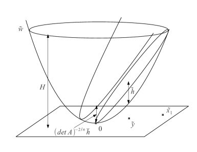
Figure 4. Lifting the tangent plane at $\tilde{y}$ by $h^{*}=\tilde{h}+\det(A)^{-2/n}\bar{h}$ we obtain a section of $\tilde{w}$ satisfying property $F$.

We now bound the volume of $S_{h^{*}}^{\tilde{w}}(\tilde{y})$ by below. Since $0,\tilde{x}_{1}$ are in this section, it has diameter at least $1$. Since $\tilde{w}$ has height $H$ it has interior Lipschitz constant $\frac{C}{H}$, so the smallest axis of the John ellipsoid for $S_{h^{*}}^{\tilde{w}}(\tilde{y})$ has length at least $c\frac{h^{*}}{H}$. We turn to the remaining axes.

Let $E_{y}$ be the John ellipsoid for $S_{\delta}^{w}(y)$. By contradiction hypothesis for any $n-2$ dimensional plane $P$ passing through the center of $E_{y}$, we can find a $n-3$ dimensional plane $P^{\prime}$ contained in $P$ such that $P^{\prime}\cap E_{y}$ is an $n-3$ dimensional ellipsoid with axes $d_{1,P^{\prime}}^{y}\geq...\geq d_{n-3,P^{\prime}}^{y}$ satisfying

$$d_{n-3,P^{\prime}}^{y}>C_{0}\delta^{1/2}|\log\delta|^{-\epsilon}.$$

Take $P$ such that $A^{-1}(P)$ is perpendicular to the segment connecting $0$ and $\tilde{x}_{1}$. By using the hypothesis and that $w$ is locally Lipschitz we have

$$d_{n-2}^{0}(h)d_{n-1}^{0}(h)>cC_{0}h^{3/2}|\log h|^{-\epsilon}.$$

Since

$$d_{1}^{0}(h)...d_{n-1}^{0}(h)<Ch^{\frac{n}{2}},$$

this gives

$$d_{1}^{0}(h)...d_{n-3}^{0}(h)<\frac{C}{C_{0}}h^{\frac{n-3}{2}}|\log h|^{\epsilon}.$$

It follows that $A^{-1}$ changes the $n-3$ dimensional volume of $P^{\prime}\cap E_{y}$ by a factor of at least

$$\frac{c(n)}{d_{1}^{0}(h)...d_{n-3}^{0}(h)}\geq cC_{0}h^{-\frac{n-3}{2}}|\log h|^{-\epsilon}.$$

Since

$$\det A>ch^{n/2}|\log h|^{-C(n)\epsilon}$$

(by the contradiction hypothesis) and $\delta=(\det A)^{2/n}h^{*}$ we conclude that

$$|S_{h^{*}}^{\tilde{w}}(\tilde{y})\cap A^{-1}(P^{\prime})|_{\mathcal{H}^{n-3}} >C_{1}\frac{(\delta^{1/2}|\log\delta|^{-\epsilon})^{n-3}}{d_{1}^{0}(h)...d_{n-3}^{0}(h)}$$

$$\geq C_{1}(h^{*})^{\frac{n-3}{2}}(\det A)^{\frac{n-3}{n}}h^{-\frac{n-3}{2}}(C|\log h|+|\log h^{*}|)^{-C(n)\epsilon}$$

for some large $C_{1}$ depending on $C_{0}$. We also have

$$H=h(\det A)^{-2/n}\leq|\log h|^{C(n)\epsilon}.$$

Using that the remaining axes have lengths at least $1$ and $c\frac{h^{*}}{H}$ we obtain

$$|S_{h^{*}}^{\tilde{w}}(\tilde{y})|>C_{1}(h^{*})^{\frac{n-1}{2}}|\log h|^{-C(n)\epsilon}(C|\log h|+|\log h^{*}|)^{-C(n)\epsilon}.$$

Using that $|S_{h^{*}}^{\tilde{w}}(\tilde{y})|<C(h^{*})^{n/2}$ we get a lower bound on $h^{*}$:

$$h^{*}>C_{1}|\log h|^{-C(n)\epsilon}.$$

(See Figure 5 for the simple case $n=3$.)

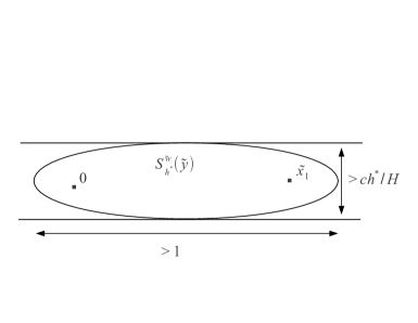
Figure 5. For the case $n=3$, the above figure implies that $|S_{h^{*}}^{\tilde{w}}(\tilde{y})|>ch^{*}/H$. This, combined with the volume estimate $|S_{h^{*}}^{\tilde{w}}(\tilde{y})|<C(h^{*})^{3/2}$ and the upper bound on $H$ from the contradiction hypothesis give a lower bound of $c|\log h|^{-C\epsilon}$ for $h^{*}$.

Recalling the definition of $h^{*}$ and using again the lower bound on $\det A$ it follows that

$$\tilde{h}+C\frac{\bar{h}}{h}|\log h|^{C(n)\epsilon}>C_{1}|\log h|^{-C(n)\epsilon}.$$

Taking $\epsilon$ to be small enough that $C(n)\epsilon=1/2$ and using that $\bar{h}|\log\bar{h}|<h$ we get

$$\tilde{h}>C_{1}|\log h|^{-1/2}.$$

Finally, let $\left(\frac{1}{2}+\gamma\right)\tilde{x_{1}}$ be the point where $\tilde{w}=\frac{H}{2}$. It is clear from convexity (see Figure 6) that

$$2\gamma H\geq\tilde{h}.$$

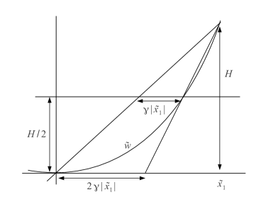
Figure 6. By convexity $2\gamma$ is at least $\tilde{h}/H$, giving a quantitative modulus of continuity for $\nabla w$ near $0$ which we exploit in Step $2$ to obtain a contradiction.

Recalling that $H<c|\log h|^{C(n)\epsilon}<c|\log h|^{1/2}$, we obtain

$$\gamma\geq C_{1}|\log h|^{-1}.$$

Let $l_{1},l_{2}$ be the distances from $0$ to the translations of $P_{1}$ and $P_{2}$ which are tangent to $\partial S_{h}^{w}(0)$ so that $b(h)\leq l_{1}+l_{2}$. The previous analysis implies that $P_{1}$ and $P_{2}$ have distance at least $\left(\frac{1}{2}+\gamma\right)l_{1}$ and $\frac{1}{2}l_{2}$ from $0$. Since $l_{1}\geq l_{2}$ it follows that

$$b(h/2)\geq\left(\frac{1}{2}+\gamma\right)l_{1}+\frac{1}{2}l_{2}\geq\left(\frac{1+\gamma}{2}\right)(l_{1}+l_{2}).$$

Since $\gamma\geq\frac{C_{1}}{|\log h|}$, step $1$ is finished.

Step 2: We iterate step 1 to prove the lemma. First assume that $\bar{h}>0$ and that $\bar{h}|\log\bar{h}|=2^{-k}$ and $h_{0}=2^{-k_{0}}$. Note that $d_{n-1}^{0}(h)>c(n)b(h)$ and that $d_{n-1}^{0}(h_{0})>c2^{-k_{0}}$ since $u$ is locally Lipschitz. Iterating step $1$ for $C_{1}$ large we obtain

$$d_{n-1}^{0}(2^{-k}) \geq c(1/2+C_{1}/k)(1/2+C_{1}/(k-1))...(1/2+C_{1}/k_{0})2^{-k_{0}}$$

$$\geq c2^{-k}\exp(C_{1}\sum_{i=k_{0}}^{k}\frac{1}{i})$$

$$\geq 2^{-k}\frac{k}{k_{0}},$$

showing that

$$d_{n-1}^{0}(\bar{h}|\log\bar{h}|)\geq c\bar{h}|\log\bar{h}|\left(|\log\bar{h}||\log h_{0}|^{-1}\right).$$

Finally, take $|\log h_{0}|=|\log\bar{h}|^{1/2}$. We conclude using convexity that

$$d_{n-1}^{0}(\bar{h})>|\log\bar{h}|^{-1}d(\bar{h}|\log\bar{h}|)>c\bar{h}|\log\bar{h}|^{1/2}.$$

Since

$$d_{1}^{0}(\bar{h})...d_{n-1}^{0}(\bar{h})<C\bar{h}^{n/2}$$

we thus have

$$d_{n-2}^{0}(\bar{h})<C\bar{h}^{1/2}|\log\bar{h}|^{-\epsilon(n)},$$

giving the desired contradiction.

In the case that $\bar{h}=0$, we may run the above iteration for any $h>0$ starting at height $h_{0}=e^{-|\log h|^{1/2}}$ to obtain the contradiction. ∎

Proof of Lemma 4.3.

First assume that $d_{1}^{y}(h)<h^{1/2}|\log h|^{-\alpha_{1}}$ for some $\alpha_{1}$. Since $|S_{h}^{w}(y)|<Ch^{n/2}$, Lemma 2.3 gives

$$Mw(S_{h}^{w}(y))>ch^{\frac{n-2}{2}}.$$

Take $C(n)$ large enough that for $r=C(n)h^{1/2}|\log h|^{-\alpha_{1}}$,

$$S_{h}^{w}(y)\subset B_{r/2}(0).$$

Clearly,

$$M\left(\frac{1}{2}|x|^{2}+w\right)(S_{h}^{w}(y))>Mw(S_{h}^{w}(y)).$$

Furthermore, $\nabla\left(u+\frac{1}{2}|x|^{2}\right)(B_{r}(0))$ contains a ball of radius $r/2$ around every point in $\nabla\left(u+\frac{1}{2}|x|^{2}\right)(S_{h}^{w}(y))$ (see Figure 7). We conclude that

$$M\left(u+\frac{1}{2}|x|^{2}\right)(B_{r}(0)) >crMw(S_{h}^{w}(y))$$

$$\geq crh^{\frac{n-2}{2}}$$

$$\geq cr^{n-1}|\log h|^{(n-2)\alpha_{1}}$$

$$\geq cr^{n-1}|\log r|^{(n-2)\alpha_{1}}.$$

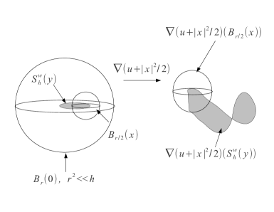
Figure 7. $\nabla(u+|x|^{2}/2)(B_{r}(0))$ contains an $r/2$-neighborhood of the surface $\nabla(u+|x|^{2}/2)(S_{h}^{w}(y))$, which projects in the $x_{n}$ direction to a set of $\mathcal{H}^{n-1}$ measure at least $cr^{n-2}|\log r|^{(n-2)\alpha_{1}}$.

We proceed inductively. Assume that $d_{i}^{y}(h)>h^{1/2}|\log h|^{-\alpha_{i}}$ for $i=1,...,k-1$ and that

$$d_{k}^{y}(h)<h^{1/2}|\log h|^{-\alpha_{k}}$$

for some $\alpha_{1},...,\alpha_{k}$ to be chosen shortly. We aim to apply Lemma 2.3 to slices of the section $S_{h}^{w}(y)$ at $0$, but we need the height of the plane $w(y)+\nabla w(y)\cdot(x-y)+h$ at $0$ to be at least $h$. We thus consider $S_{2h}^{w}(y)$ instead. Note that $d_{i}^{y}(2h)>h^{1/2}|\log h|^{-\alpha_{i}}$ for $i\leq k-1$ and by convexity $d_{k}^{y}(2h)<2h^{1/2}|\log h|^{-\alpha_{k}}$.

Rotate so that the axes align with those for the John ellipsoid of $S_{2h}^{w}(y)$. Take the restriction of $w$ to the subspace spanned by $e_{k},...,e_{n-1}$, and call this restriction $w_{k}$. Let

$$S^{w_{k}}=S_{2h}^{w}(y)\cap\{x_{1}=...=x_{k-1}=0\},$$

the slice of the section $S_{2h}^{w}(y)$ in this subspace. Then since

$$d_{1}^{y}(2h)...d_{n-1}^{y}(2h)\leq Ch^{\frac{n}{2}},$$

by hypothesis we have

$$|S^{w_{k}}|_{\mathcal{H}^{n-k}}\leq Ch^{\frac{n+1-k}{2}}|\log h|^{\alpha_{1}+...+\alpha_{k-1}}.$$

Since $S_{h}^{w}(y)$ contains $0$ and $S^{w_{k}}$ is the slice of $S_{2h}^{w}(y)$, we know that $w_{k}$ has height at least $h$ in $S^{w_{k}}$. Using this and Lemma 2.3,

$$Mw_{k}(S^{w_{k}})\geq ch^{\frac{n-k-1}{2}}|\log h|^{-(\alpha_{1}+...+\alpha_{k-1})}.$$

Finally, take $C(n)$ large enough that for $r=C(n)h^{1/2}|\log h|^{-\alpha_{k}}$ we have

$$S^{w_{k}}\subset B_{r/2}(0).$$

By strict quadratic growth, $\nabla\left(u+\frac{1}{2}|x|^{2}\right)(B_{r}(0))$ contains a ball of radius $r/2$ around every point in $\nabla(u+\frac{1}{2}|x|^{2})(S^{w_{k}})$. It follows that

$$M\left(u+\frac{1}{2}|x|^{2}\right)(B_{r}(0)) \geq cMw_{k}(S^{w_{k}})r^{k}$$

$$\geq ch^{\frac{n-k-1}{2}}|\log h|^{-(\alpha_{1}+...+\alpha_{k-1})}r^{k}$$

$$\geq cr^{n-1}|\log r|^{(n-k-1)\alpha_{k}-(\alpha_{1}+...+\alpha_{k-1})}.$$

Choose $\beta_{i}$ so that $(n-k-1)\beta_{k}-(\beta_{1}+...+\beta_{k-1})=1$ and let $\alpha_{i}=c\beta_{i}$, with $c$ chosen so that $\alpha_{n-2}=\epsilon$. If $d_{1}^{y}(h)<h^{1/2}|\log h|^{-\alpha_{1}}$, we are done by the first step, so assume not. Then apply the inductive step for $i=2,...,n-2$ to conclude the proof. ∎

5. Example

In this section we construct a solution to $\det D^{2}u=1$ in $\mathbb{R}^{3}$ such that $\Sigma$ has Hausdorff dimension exactly $2$. A small modification gives the analagous example in $\mathbb{R}^{n}$ with a singular set of Hausdorff dimension $n-1$. This shows that the estimate on the Hausdorff dimension of the singular set in [M] cannot be improved to $n-1-\delta$ for any $\delta$.

We proceed in several steps:

1. The key step is to construct a subsolution $w$ in $\mathbb{R}^{3}$ satisfying $\det D^{2}w\geq 1$ that degenerates along $\{x_{1}=x_{2}=0\}$ and grows logarithmically faster than quadratic in the $x_{1}$ direction, in particular like $x_{1}^{2}|\log x_{1}|^{4}$.

2. Next, we construct $S\subset[-1,1]$ of Hausdorff dimension $1$ and a convex function $v$ on $[-1,1]$ such that $v$ separates from its tangent line faster than $r^{2}|\log r|^{4}$ at each point in $S$.

3. Finally, we obtain our example by solving the Dirichlet problem

   $$\det D^{2}u=1\quad\text{ in }\Omega=\{|x^{\prime}|<1\}\times(-1,1),\quad\quad u|_{\partial\Omega}=C(v(x_{1})+|x_{2}|)$$

   and comparing with $w$ at points in $S\times\{0\}\times\{\pm 1\}$.

In the following analysis $c,C$ will denote small and large constants respectively.

Construction of $w$: We first seek a function with just faster than quadratic growth in one direction and sections $S_{h}(0)$ with volume smaller than $h^{3/2}$. To that end, let

$$g(x_{1},x_{2})=x_{1}^{2}|\log x_{1}|^{\alpha}+\frac{|x_{2}|}{|\log x_{2}|^{\beta}}$$

for some $\alpha,\beta$ to be chosen shortly. It is tempting to guess $w=g(x_{1},x_{2})(1+x_{3}^{2})$. However, the dominant terms in the determinant of the Hessian near the $x_{2}$ axis are

$$\frac{|\log x_{1}|^{\alpha}}{|\log x_{2}|^{2\beta}}\left(\frac{1}{|\log g|}-x_{3}^{2}\right),$$

where the first comes from the diagonal entries and the second from the mixed derivatives. Thus, this function is not convex. This motivates the following modification:

$$w(x^{\prime},x_{3})=g(x^{\prime})\left(1+\frac{x_{3}^{2}}{|\log g(x^{\prime})|}\right).$$

It is straightforward to check that the leading terms in the determinant of the Hessian (taking $x_{3}$ small) are

$$\frac{x_{1}^{2}|\log x_{1}|^{2\alpha}}{|x_{2}(\log x_{2})^{\beta+1}\log g|}+\frac{|\log x_{1}|^{\alpha}}{|(\log x_{2})^{1+2\beta}\log g|},$$

since now the mixed derivative terms have the same homogeneity in $\log(g)$ as the diagonal terms. For $|x^{\prime}|$ small, the first term is large in $\{|x_{2}|<|x_{1}|^{3}\}$, and by taking $\alpha=2+2\beta$ the second term is bounded below by a positive constant in $\{|x_{2}|\geq|x_{1}|^{3}\}$. Thus, up to rescaling and multiplying by a constant we have

$$\det D^{2}w\geq 1$$

in $\Omega=\{|x^{\prime}|<1\}\times(-1,1)$. For convenience, we take $\beta=1$ and $\alpha=4$ for the rest of the example.

Construction of $S$: Start with the interval $[-1/2,1/2]$. For the first step remove an open interval of length $\frac{5}{6}$ from the center. At the $k^{th}$ step, remove intervals a fraction $\frac{5}{k+5}$ of the length of the remaining $2^{k}$ intervals from their centers. Denote the centers of the removed intervals by $\{x_{i,k}\}_{i=1}^{2^{k}}$, and the intervals by $I_{i,k}$. Finally, let

$$S=[-1,1]-\cup_{i,k}I_{i,k}.$$

Let $l_{k}=|I_{i,k}|$. It is easy to check

$$l_{k} =\frac{10}{k+5}2^{-k}\left(1-\frac{5}{k+4}\right)...\left(1-\frac{5}{6}\right)$$

$$\leq\frac{C}{k^{6}}2^{-k}.$$

One checks similarly that the length of the remaining intervals after the $k^{th}$ step is at least

$$2^{-k}k^{-15}.$$

It follows that

(2) $$\inf\left\{\sum_{i=1}^{\infty}r_{i}|\log(r_{i})|^{15}:\{B_{r_{i}}(x_{i})\}\text{ cover }S,r_{i}<\delta\right\}>c$$

for all $\delta>0$. In particular, the Hausdorff dimension of $S$ is exactly $1$.

Construction of $v$: Let

$$f(x)=\left\{\begin{array}[]{ll}|x|&\quad|x|\leq 1\\ 2|x|-1&\quad|x|>1\end{array}\right.$$

We add rescalings of $f$ together to produce the desired function:

$$v(x)=\sum_{k=1}^{\infty}k^{4}l_{k}^{2}f(l_{k}^{-1}(x-x_{i,k})).$$

We now check that $v$ satisfies the desired properties:

1. v is convex, as the sum of convex functions. Furthermore, using that $l_{k}<C2^{-k}k^{-6}$ we have

   $$|v(x)| \leq C\sum_{k=1}^{\infty}\sum_{i=1}^{2^{k}}k^{4}l_{k}$$

   $$\leq C\sum_{k=1}^{\infty}k^{-2}$$

   $$\leq C$$

   so $v$ is bounded.

2. Let $x\in S$. We aim to show that $v$ separates from a tangent line more than $r^{2}|\log(r)|^{4}$ a distance $r$ from $x$. By subtracting a line assume that $v(x)=0$ and that $0$ is a subgradient at $x$. Assume further that $x+r<1/2$ and that $l_{k}<r\leq l_{k-1}$. There are two cases to examine:

   Case 1: There is some $y\in(x+r/2,x+r)\cap S$. Then by the construction of $S$ it is easy to see that there is some interval $I_{i,k}$ such that $I_{i,k}\subset(x,x+r)$. On this interval, $v$ grows by

   $$k^{4}l_{k}^{2}\geq cl_{k}^{2}|\log(l_{k})|^{4}\geq cr^{2}|\log(r)|^{4}.$$

   Case 2: Otherwise, there is an interval $I_{i,j}$ of length exceeding $r/2$ such that $(x+r/2,x+r)\subset I_{i,j}$. Then at the left point of $I_{i,j}$, the slope of $v$ jumps by at least $k^{4}l_{k}$. It follows that at $x+r$, $v$ is at least

   $$crk^{4}l_{k}\geq cr^{2}|\log(r)|^{4}.$$

   Thus, $v$ has the desired properties.

Construction of $u$: We recall the following lemma on the solvability of the Monge-Ampère equation (see [Gut]).

Lemma 5.1.

If $\Omega$ is open and convex, $\mu$ is a finite Borel measure and $\varphi$ is continuous on $\partial\Omega$ then there exists a unique convex solution $u\in C(\bar{\Omega})$ to the Dirichlet problem

$$\det D^{2}u=\mu,\quad u|_{\partial\Omega}=\varphi.$$

Let $\varphi(x_{1},x_{2},x_{3})=C(v(x_{1})+|x_{2}|)$ for a constant $C$ we will choose shortly, and obtain $u$ by solving the Dirichlet problem

$$\det D^{2}u=1\quad\text{ in }\Omega=\{|x^{\prime}|<1\}\times[-1,1],\quad\quad u|_{\partial\Omega}=\varphi.$$

Take $x\in S\times\{0\}\times\{\pm 1\}$. By translating and subtracting a linear function assume that $x_{1}=0$ and $0$ is a subgradient for $\varphi$ at $x$. Taking $C$ large we guarantee that

$$\varphi(x_{1},x_{2},\pm 1)>C(x_{1}^{2}|\log(x_{1})|^{4}+|x_{2}|)>w(x_{1},x_{2},\pm 1)$$

for all $x_{1},x_{2}$, and that that $\varphi>w$ on the sides of $\Omega$. Thus, $u\geq w$ in all of $\Omega$. Since $u=0$ at both $(0,0,\pm 1)$ and $w(0,0,x_{3})=0$ for all $|x_{3}|<1$, we have by convexity that $u=0$ along $(0,0,x_{3})$.

This shows that for these examples

$$\Sigma\subset S\times\{0\}\times(-1,1),$$

which has Hausdorff dimension exactly $2$.

Remark 5.2.

To get the analagous example in $\mathbb{R}^{n}$, take

$$u(x_{1},x_{2},x_{3})+x_{4}^{2}+...+x_{n}^{2}.$$

6. Optimality of Theorem 1.1

In [M] we construct for any $\epsilon$ solutions to $\det D^{2}u=1$ in $\mathbb{R}^{n}$ that are not in $W^{2,1+\epsilon}$, but as $\epsilon\rightarrow 0$ these examples blow up. In this section we aim to improve this by showing that the example in the previous section is not in $W^{2,1+\epsilon}$ for any $\epsilon$, and in fact the second derivatives are not in $L\log^{M}L$ for $M$ large.

Let $\phi(x)=(1+x)(\log(1+x))^{M}$ for some $M$ large. Then $\phi$ is convex for $x\geq 0$, so for any nonnegative integrable function $f$ and ball $B_{r}$ we have by Jensen’s inequality that

$$\int_{B_{r}}\phi(r^{n}f(x))\,dx\geq cr^{n}\phi\left(\int_{B_{r}}f(x)\,dx\right).$$

Taking $f(x)=r^{-n}\Delta u(x)$ we obtain

$$\int_{B_{r}}(1+\Delta u)(\log(1+\Delta u))^{M}\,dx\geq c\left(\int_{B_{r}}\Delta u\,dx\right)\left(\log\left(r^{-n}\int_{B_{r}}\Delta u\,dx\right)\right)^{M}.$$

Recall that at points $x\in S\times\{0\}\times(-1,1)^{n-2}$ the subsolutions $w$ touch $u$ by below, and that $w$ grows like $|x_{2}||\log x_{2}|^{-1}$ at $x$. It follows that

$$\sup_{\partial B_{r}(x)}(u-u(x))\geq cr|\log r|^{-1}.$$

Applying convexity we conclude that

$$\int_{B_{r}(x)}(1+\Delta u)\left(\log(1+\Delta u)\right)^{M}\,dx \geq c\left(\int_{\partial B_{r}(x)}u_{\nu}\right)\left(\log\left(r^{-n}\int_{\partial B_{r}(x)}u_{\nu}\right)\right)^{M}$$

$$\geq cr^{n-1}|\log r|^{-1}\left(\log(cr^{-1}|\log(r)|^{-1})\right)^{M}$$

$$\geq cr^{n-1}|\log r|^{M-1}.$$

Cover $\Sigma\cap B_{1/2}$ with balls of radius less than $\delta$ and take a Vitali subcover $\{B_{r_{i}}\}_{i=1}^{N}$. We then have

$$\int_{B_{1/2}}(1+\Delta u)\left(\log(1+\Delta u)\right)^{M}\,dx\geq c\sum_{i=1}^{N}r_{i}^{n-1}|\log r_{i}|^{M-1},$$

and for $M$ large the right side goes to $\infty$ as $\delta\rightarrow 0$ by equation 2.

Thus, the second derivatives of $u$ are not in $L\log^{M}L$ for $M$ large, and in particular $u$ is not in $W^{2,1+\epsilon}$ for any $\epsilon$.

References

- [C1] L. Caffarelli, A localization property of viscosity solutions to the Monge-Ampère equation and their strict convexity, Ann. of Math. 131 (1990), 129-134.
- [C2] L. Caffarelli, Interior estimates for solutions of Monge-Ampère equation, Ann. of Math. 131 (1990), 135-150.
- [CG] L. Caffarelli and C. Gutierrez, Properties of solutions of the linearized Monge-Ampère equation, Amer. J. Math 119 (1997), 423-465.
- [DF] G. De Philippis and A. Figalli, regularity for solutions of the Monge-Ampère equation, Invent. Math. 192 (2013), 55-69.
- [DFS] G. De Philippis, A. Figalli and O. Savin, A note on interior estimates for the Monge-Ampère equation, Math. Ann. 357 (2013), 11-22.
- [Gut] C. Gutierrez, “The Monge-Ampère Equation,” Progress in Nonlinear Differential Equations and their Applications 44, Birkhäuser Boston, Inc., Boston, MA, 2001.
- [M] C. Mooney, Partial regularity for singular solutions to the Monge-Ampère equation, Comm. Pure Appl. Math., to appear.
- [W] X.-J. Wang, Regularity for Monge-Ampère equation near the boundary, Analysis 16 (1996) 101-107.