Kepler-77b: a very low albedo, Saturn-mass transiting planet
around a metal-rich solar-like star ^,,

We report the discovery of Kepler-77b (alias KOI-127.01), a Saturn-mass transiting planet in a 3.6-day orbit around a metal-rich solar-like star. We combined the publicly available Kepler photometry (quarters 1–13) with high-resolution spectroscopy from the Sandiford@McDonald and FIES@NOT spectrographs. We derived the system parameters via a simultaneous joint fit to the photometric and radial velocity measurements. Our analysis is based on the Bayesian approach and is carried out by sampling the parameter posterior distributions using a Markov chain Monte Carlo simulation. Kepler-77b is a moderately inflated planet with a mass of M_p $=0.430\pm 0.032$ $\mathrm{M}_{\mathrm{Jup}}$, a radius of R_p $=0.960\pm 0.016$ $\mathrm{R}_{\mathrm{Jup}}$, and a bulk density of $\rho_{\mathrm{p}}=0.603\pm 0.055$  g cm^-3. It orbits a slowly rotating ($P_{\mathrm{rot}}=36\pm 6$ days) G5 V star with $M_{\star}=0.95\pm 0.04$ $M_{\odot}$, $R_{\star}=0.99\pm 0.02$ $R_{\odot}$, $T_{\mathrm{eff}}$ $=5520\pm 60$ K, [M/H] $=0.20\pm 0.05$ dex, that has an age of $7.5\pm 2.0$ Gyr. The lack of detectable planetary occultation with a depth higher than $\sim$10 ppm implies a planet geometric and Bond albedo of $A_{\mathrm{g}}\leq 0.087\pm 0.008$ and $A_{\mathrm{B}}\leq 0.058\pm 0.006$, respectively, placing Kepler-77b among the gas-giant planets with the lowest albedo known so far. We found neither additional planetary transit signals nor transit-timing variations at a level of $\sim$0.5 minutes, in accordance with the trend that close-in gas giant planets seem to belong to single-planet systems. The 106 transits observed in short-cadence mode by Kepler for nearly 1.2 years show no detectable signatures of the planet’s passage in front of starspots. We explored the implications of the absence of detectable spot-crossing events for the inclination of the stellar spin-axis, the sky-projected spin-orbit obliquity, and the latitude of magnetically active regions.

1 Introduction

Space-based transit surveys are opening up a new exciting era in exoplanetary science, enlarging the known parameter space of planetary systems. The high-precision, long-term, and uninterrupted photometry from CoRoT (Baglin et al. 2006) and Kepler (Borucki et al. 2010) enables us to detect transiting planets down to the Earth- and Mercury-like regime (e.g., CoRoT-7b, Leger et al. 2009; Kepler-10b, Batalha et al. 2011; Kepler-37b Barclay et al. 2013), planets in long-period orbits (e.g., CoRoT-9b, Deeg et al. 2010), planets in the habitable zone (e.g., Kepler-22b, Borucki et al. 2012), multi-transiting systems (e.g., CoRoT-24, Alonso et al. 2012; Kepler-11, Lissauer et al. 2011), and circumbinary systems (e.g., Kepler-16, Doyle et al. 2011; Kepler-47, Orosz et al. 2012). The exquisite photometry from space, combined with ground-based spectroscopy, enables us to derive the most precise planetary and stellar parameters to date, which in turn are essential for investigating the internal structure, formation, and migration of planets.

Based upon the analysis of the first sixteen months of Kepler photometry, Batalha et al. (2013) have recently announced 2321 transiting planet candidates (Kepler Object of Interests, KOIs), almost doubling the number of candidates previously published by Borucki et al. (2010). Although those objects have been accurately vetted for astrophysical false-positives using Kepler photometry (see, e.g., Sect. 4 in Batalha et al. 2013), many of them - especially those where only a single planet is observed to transit - remain planetary candidates and deserve additional investigations, including high-resolution spectroscopy and radial velocity (RV) measurements. Different configurations involving eclipsing binary systems can indeed mimic a transit-like signal (Brown 2003), and can only be weeded out with ground-based follow-up observations. Given the large number of KOIs, the Kepler team is currently focusing its spectroscopic follow-up effort on the smallest planets, while relying on the rest of the scientific community to confirm the remaining planetary objects. Ground-based observations (e.g., Colón et al. 2012; Lillo-Box et al. 2012; Santerne et al. 2012) have recently proven that the false-positive rate of Kepler transiting candidates might be noticeably higher than the 5 % previously claimed by Morton & Johnson (2011), proving the need for more investigations to assess the real nature of these objects.

We herein announce the discovery of the Kepler transiting planet Kepler-77b (also known as KOI-127.01), a Saturn-mass gas giant planet orbiting a metal-rich solar-like star. We combined Kepler public photometry with high-resolution spectroscopy carried out with Sandiford@McDonald-2.1m and FIES@NOT to confirm the planetary nature of the transiting object and derive the system parameters.

The paper is structured as follows. In Sect. 2, we describe the Kepler data available at the time of writing. In Sect. 3, we report on our high-resolution spectroscopic follow-up of Kepler-77. In Sect. 4, we present the properties of the planet’s host star. In Sect. 5, we simultaneously model the photometric and spectroscopic data using a Bayesian-based model approach. Finally, in Sect. 6, we present the fundamental parameters of Kepler-77b, look for additional companions in the system, constrain the planet’s albedo, and explore the limits placed by the apparent absence of spot-crossings on the inclination of the stellar spin-axis, the sky-projected spin-orbit obliquity, and the latitude of magnetically active regions.

2 Kepler photometry

Table 1: Kepler, KOI, GSC2.3, USNO-A2, and 2MASS identifiers of the planet-hosting star Kepler-77. Equatorial coordinates and optical SDSS-$g$,-$r$,-$i$,-$z$ photometry are from the Kepler Input Catalogue. Infrared $J$,$H$,$Ks$ and $W1$,$W2$,$W3$,$W4$ data are taken from the 2MASS (Cutri et al. 2003) and WISE (Wright et al. 2010) database, respectively.

Main identifiers
Kepler ID	8359498
KOI ID	127
GSC2.3 ID	N2K0000444
USNO-A2 ID	1275-11111739
2MASS ID	19182590+4420435
Equatorial coordinates
RA  (J2000)	$19^{h}\,18^{m}\,25\aas@@fstack{s}910$
Dec (J2000)	$+44\hbox{${}^{\circ}$}\,20\arcmin\,43\aas@@fstack{\prime\prime}51$
Magnitudes
Filter   ($\lambda_{\mathrm{e}ff}$)	Mag	Error
$g$     ( 0.48 $\mu m$)	14.449	0.030
$r$     ( 0.63 $\mu m$)	13.871	0.030
$i$     ( 0.77 $\mu m$)	13.720	0.030
$z$     ( 0.91 $\mu m$)	13.658	0.030
$J$     ( 1.24 $\mu m$)	12.758	0.023
$H$    ( 1.66 $\mu m$)	12.444	0.019
$Ks$  ( 2.16 $\mu m$)	12.361	0.018
$W_{1}$  ( 3.35 $\mu m$)	12.309	0.023
$W_{2}$  ( 4.60 $\mu m$)	12.377	0.023
$W_{3}$  (11.56 $\mu m$)	$12.587^{a}$	-
$W_{4}$  (22.09 $\mu m$)	$\leavevmode\nobreak\ \leavevmode\nobreak\ 9.492^{a}$	-

Kepler-77, whose main designations, equatorial coordinates, and optical and infrared photometry are reported in Table 1, was previously identified as a Kepler planet-hosting star candidate by Borucki et al. (2010) and Batalha et al. (2013) and listed as KOI-127. Speckle observations (Howell et al. 2011) and adaptive optics imaging (Adams et al. 2012) excluded a background eclipsing binary spatially close to the star.

At the time of writing, the public Kepler data for Kepler-77, i.e. quarters 1–13 (Q₁–Q₁₃), consist of more than three years of nearly continuous observations, from 13 May 2009 to 27 June 2012. Two hundred and ninety-eight planetary-like transits were observed with a long-cadence (LC) sampling time of $T_{\mathrm{exp}}$=1765.5 sec. One hundred and six transits were also observed with a short-cadence (SC) sampling time of $T_{\mathrm{exp}}$=58.89 sec, from quarter 3 (Q₃) to quarter 7 (Q₇).

The photometric data were automatically processed with the new version of the Kepler pre-search data conditioning (PDC) pipeline (Stumpe et al. 2012), which uses a Bayesian maximum a posteriori (MAP) approach to remove the majority of instrumental artefacts and systematic trends (Smith et al. 2012). Clear outliers and photometric discontinuities across the data gaps that coincide with the quarterly rolls of the spacecraft were removed by visual inspection of the PDC-MAP light curve. We performed a test analysis of the aperture photometry produced by the Kepler pipeline, with and without using the PDC-MAP. We found that the data reduction performed by the automatic pipeline does not affect the planet characterisation for the current case and we used the PDC-MAP light curve for our analysis (Sect. 5). The point-to-point scatter estimates for the PDC-MAP LC and SC data are 378 and 1398 ppm, respectively (Sect. 5).

Figure 1 shows the cleaned PDC-MAP Kepler LC light curve of Kepler-77. The data from different quarters were stitched together by arbitrarily normalising the flux by the out-of-transit median value per quarter. The $\sim$1%-deep transit signals are visible, along with a $\sim$0.4 % (peak-to-peak) out-of-transit variability whose nature is discussed in Sect. 4.4.

Figure 1: Q₁ – Q₁₃ Kepler LC light curve of Kepler-77. The data from different quarters have been stitched together by arbitrarily normalising the flux by the out-of-transit median value per quarter. The points around normalised flux $\sim$0.99 mark the bottom of the 298 transits observed in LC mode. The light curve shows an out-of-transit flux variations with a peak-to-peak amplitude of $\sim$0.4 %.

3 High-resolution spectroscopy

3.1 Sandiford observations

We performed reconnaissance high-resolution spectroscopy with the Sandiford Échelle spectrometer (McCarthy et al. 1993) attached at the Cassegrain focus of the 2.1-m telescope of the McDonald Observatory (Texas, USA). Four spectra were acquired at different epochs in May 2011, under clear and stable sky conditions. Three out of four observations were scheduled around orbital phases 0.25 and 0.75, i.e., when the highest amplitude of the RV curve is expected, to efficiently weed out an eclipsing binary scenario. We used the $1\arcsec$ slit width, which yields a resolving power of $R=47\,000$. As the size of the CCD can cover only $\sim$1000 Å, we set the spectrograph grating angle to encompass the wavelength range 5000–6000 Å. Taking into account the brightness of the target star, this was a good compromise between signal-to-noise (S/N) ratio and number of photospheric lines, which are suitable for RV measurements and reconnaissance spectral analysis. Three consecutive exposures of 1200 sec were taken during each epoch observation to properly remove cosmic ray hits. We followed the observing strategy described in Buchhave et al. (2010), i.e., we traced the RV drift of the instrument by acquiring long-exposed (T_exp=30 sec) ThAr spectra right before and after each epoch observation. The data were reduced using a customised IDL software suite, which includes bias subtraction, flat fielding, order tracing and extraction, and wavelength calibration. Radial velocity measurements were derived performing a multi-order cross-correlation with the RV standard star HD 182572 (Udry et al. 1999).

The Sandiford spectra revealed that Kepler-77 is a slowly rotating solar-like star. A first estimate of the photospheric parameters was made by using a modified version of the spectral analysis technique described in Gandolfi et al. (2008), which is based on the use of a grid of stellar templates to simultaneously derive spectral type, luminosity class, and interstellar reddening from flux-calibrated low-resolution spectra. We modified the code to compare the co-added and normalised Sandiford spectrum with a grid of synthetic model spectra from Castelli & Kurucz (2004), Coelho et al. (2005), and Gustafsson et al. (2008). We found that Kepler-77 is a G5 V star, with an effective temperature $T_{\mathrm{eff}}$ $=5500\pm 100$ K, surface gravity log g $=4.50\pm 0.10$ dex, metallicity [M/H] $=0.20\pm 0.10$ dex, and a projected rotational velocity $v$ sin $i_{\star}$ $\approx 2$ kms, in agreement with the photospheric parameters listed in the Kepler input catalogue.

The Sandiford RV measurements are listed in Table 2, along with the cross-correlation function (CCF) bisector spans, and the S/N ratio per pixel at 5500 Å. The reconnaissance Sandiford data reject a binary system scenario and are consistent with an RV variation of semi-amplitude $K\,\approx\,60$  m s^-1 in phase with the Kepler ephemeris (Fig. 2). Assuming a mass of $M_{\star}\,\approx\,1$ $M_{\odot}$ for the central star, as reported in the Kepler input catalogue, the RV semi-amplitude is compatible with a companion mass of M_p $\approx\,0.5$ $\mathrm{M}_{\mathrm{Jup}}$.

Table 2: Sandiford and FIES radial velocity measurements of Kepler-77. The CCF bisector spans and the S/N ratio per pixel at 5500 Å are listed in the last two columns.

HJD	RV	$\sigma_{\mathrm{R}V}$	Bisector	S/N/pixel
($-$ 2 450 000)	km s-1	km s-1	km s-1	@5500 Å
Sandiford
5701.82595	$-$24.862	0.042	$-$0.032	16.2
5703.80604	$-$24.742	0.034	0.001	18.6
5704.93367	$-$24.818	0.042	0.011	15.4
5705.78525	$-$24.810	0.026	$-$0.004	22.2
FIES
6101.69609	$-$24.773	0.018	0.039	17.2
6102.53160	$-$24.808	0.018	0.002	20.8
6104.60191	$-$24.712	0.024	0.006	12.1
6105.60914	$-$24.805	0.020	$-$0.003	11.7
6107.70122	$-$24.691	0.019	$-$0.018	15.8
6118.65614	$-$24.705	0.014	0.028	20.5
6119.70464	$-$24.803	0.012	$-$0.024	24.2
6121.66698	$-$24.716	0.014	0.006	25.0
6122.70204	$-$24.702	0.023	0.067	11.1
6202.41791	$-$24.806	0.012	0.019	28.6
6214.34702	$-$24.739	0.024	$-$0.022	11.2

3.2 FIES observations

The promising results obtained with Sandiford prompted us to continue the spectroscopic follow-up of Kepler-77. Eleven additional high-resolution spectra were obtained at different epochs, between June and October 2012, using the FIbre-fed Échelle Spectrograph (FIES; Frandsen & Lindberg 1999) mounted at the 2.56-m Nordic Optical Telescope (NOT) of Roque de los Muchachos Observatory (La Palma, Spain). The observations were carried out under clear sky conditions, with seeing typically varying between 0.6 and 1.5 ″. We used the high-res $1.3\,\arcsec$ fibre, which provides a resolving power of R=67 000 and a wavelength coverage of about 3600–7400 Å. We adopted the same calibration scheme and exposure time as for the Sandiford follow-up. Observations were first scheduled around quadrature, to validate the trend inferred with Sandiford. Once the RV variation was confirmed, FIES RVs measurements were secured at different orbital phases to evenly cover the RV curve. The data were reduced in the same fashion as the Sandiford spectra. Once more, HD 182572 was used as the RV standard star.

The FIES RV measurements, CCF bisector spans, and S/N ratio per pixel at 5500 Å are listed in Table 2. The upper panel of Figure 2 shows the phase-folded RV curve of Kepler-77, as obtained from the global analysis of the photometric and spectroscopic data described in Sect. 5.

Following the method outlined in Queloz et al. (2001), we performed an analysis of the Sandiford and FIES CCF bisector spans to exclude the presence of periodic distortions in the spectral line profile that might be caused either by stellar magnetic activity (i.e., photospheric spots and plages), or by a blended eclipsing binary whose light is diluted by Kepler-77. The lack of correlation between the CCF bisector span and RV data (Fig. 2, lower panel) proves that the Doppler shift observed in Kepler-77 are induced by the companion’s orbital motion.

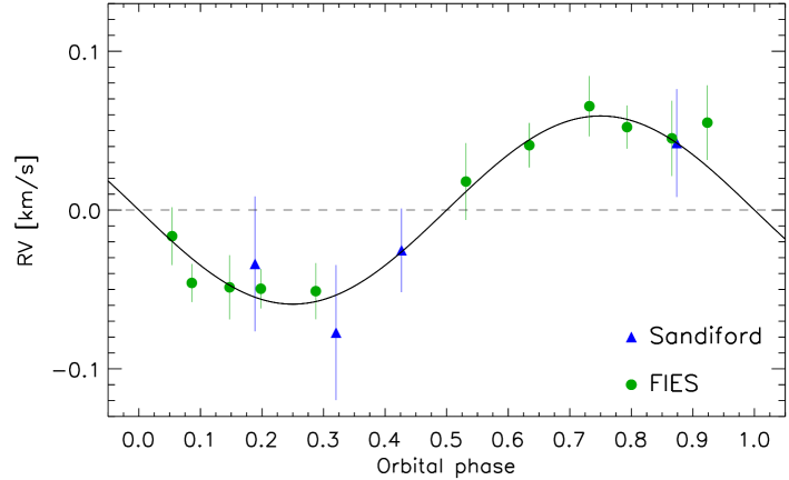
Figure 2: Upper panel: Sandiford and FIES radial velocities measurements of Kepler-77 and Keplerian fit to the data. The systemic velocities for each instrument, as derived from the global modelling of the data (Sect. 5 and Table 6), have been subtracted from the RV measurements. Lower panel: Bisector spans of the Sandiford and FIES cross-correlation functions versus RV measurements, after subtracting the systemic velocities. The error bars in the CCF bisector spans are taken to be twice the uncertainties in the RV data.

4 Properties of the parent star

4.1 Photospheric parameters

An improvement on the determination of the photospheric parameters of Kepler-77 was achieved using the co-added FIES spectrum, which has a S/N ratio of about 65 per pixel at 5500 Å. We used the same procedure outlined in Sect. 3.1, as well as the spectral analysis package SME 2.1 (Valenti & Piskunov 1996; Valenti & Fischer 2005) and the ROTFIT code from Frasca et al. (2003, 2006). The latter is based on the use of ELODIE archive spectra of standard stars with well-known parameters (Prugniel & Soubiran 2001). The three methods provided consistent results within the error bars. The microturbulent $v_{\mathrm{micro}}$ and macroturbulent $v_{\mathrm{macro}}$ velocities were derived using the calibration equations of Bruntt et al. (2010) for Sun-like dwarf stars. The projected rotational velocity $v$ sin $i_{\star}$ was measured by fitting the profile of several clean and unblended metal lines. The final adopted values are $T_{\mathrm{eff}}$ $=5520\pm 60$ K, log g$=4.40\pm 0.10$ dex, [M/H] $=0.20\pm 0.05$ dex, $v_{\mathrm{micro}}=0.9\pm 0.1$  km s^-1, $v_{\mathrm{macro}}=1.8\pm 0.3$  km s^-1, and $v$ sin $i_{\star}$ $=1.5\pm 1.0$  km s^-1, in very good agreement with the values derived from the Sandiford spectra and those reported in the Kepler input catalogue.

4.2 Stellar mass, radius, and age

We determined the mass $M_{\star}$ and radius $R_{\star}$ of the planet-hosting star Kepler-77 using the spectroscopically derived effective temperature $T_{\mathrm{eff}}$ and metallicity [M/H], along with the bulk stellar density $\rho_{\star}$, as obtained from the transit light curve modeling (Sect. 5). We compared the position of the star on a $\rho_{\star}$ versus $T_{\mathrm{eff}}$ diagram with a grid of ad hoc evolutionary tracks.

Stellar models were generated using an updated version of the FRANEC code (Degl’Innocenti et al. 2008; Tognelli et al. 2011) and adopting the same input physics and parameters as those used in the Pisa Stellar Evolution Data Base for low-mass stars (see, e.g., Dell’Omodarme et al. 2012, for a detailed description). To account for the current photospheric metallicity of Kepler-77 ([M/H] $=0.20\pm 0.05$ dex) and microscopic diffusion of heavy elements towards the centre of the star (see below), we computed evolutionary tracks assuming an initial metal content of Z=0.0178, Z=0.0198, Z=0.0221, Z=0.0245, Z=0.0272, and Z=0.0301. The corresponding initial helium abundances (i.e., Y=0.284, 0.288, 0.293, 0.297, 0.303, and 0.308) were determined assuming a helium-to-metal enrichment ratio $\Delta$Y/$\Delta$Z=2 (Jimenez et al. 2003; Casagrande 2007; Gennaro et al. 2010) and a cosmological ⁴He abundance Y_p=0.2485 (Cyburt 2004; Peimbert et al. 2007a, b). For each chemical composition, we generated a very fine grid of evolutionary tracks in the mass domain $M_{\star}=0.80$–$1.10$ $M_{\odot}$, with step of $\Delta M_{\star}=0.01$ $M_{\odot}$. Thus, a total of 186 stellar tracks were calculated specifically for this project.

As mentioned, the models take into account microscopic diffusion, where diffusion velocities for the different chemical species due to gravitational settling and thermal diffusion are calculated by means of the routine developed by Thoul et al. (1994). Due to this effect, the surface chemical composition changes with time depending on the stellar mass. As a consequence, the metallicity currently observed on the surface of low-mass main-sequence stars is different from the original one, a difference that increases with the age. To improve the inferred stellar parameters resulting from the comparison between models and observational data, the effect of this change in the surface chemical composition has to be taken into account, as far as old low-mass main-sequence stars are analysed.

To reproduce the current surface metallicity measured for Kepler-77, we found that evolutionary tracks with initial metal content between Z=0.0221 and Z=0.0272 had to be used. We derived a mass of $M_{\star}=0.95\pm 0.04$ $M_{\odot}$  a radius of $R_{\star}=0.99\pm 0.02$ $R_{\odot}$  and an age of $7.5\pm 2.0$ Gyr (Table 6). Stellar mass and radius translate into a surface gravity of log g $=4.42\pm 0.01$ dex, which agrees very well with the spectroscopically derived value (log g $=4.40\pm 0.10$ dex). We note that assuming an initial metal content equal to the measured current value would lead to an underestimate of the stellar mass and radius of about 0.04 $M_{\odot}$ and 0.01 $R_{\odot}$  respectively, as well as an overestimate of the age of about 2 Gyr.

We also used Equation 32 from Barnes (2010) and the rotation period of the star ($P_{\mathrm{rot}}=36\pm 6$ days; see Sect. 4.4) to infer the gyro-age of Kepler-77, assuming a convective turnover time-scale of $\tau_{\mathrm{c}}=41.40$ days (Barnes & Kim 2010) and a zero-age main-sequence rotation period of $P_{0}=1.1$ days (Barnes 2010). We found a gyro-age of $7.3\pm 2.4$ Gyr, in very good agreement with the value obtained from the evolutionary tracks.

4.3 Interstellar extinction and distance

The interstellar extinction $A_{\mathrm{v}}$ and spectroscopic distance $d$ to Kepler-77 were obtained by applying the method described in (Gandolfi et al. 2010). Briefly, we simultaneously fitted the available SDSS, 2MASS, and WISE colours (Table 1) with synthetic theoretical magnitudes. These were obtained by integrating a NextGen model spectrum (Hauschildt et al. 1999) - with the same photospheric parameters as the star - over the response curve of the SDSS, 2MASS, and WISE photometric systems. We excluded the $W_{3}$ and $W_{4}$ WISE magnitudes, which are only upper limits. Assuming a normal extinction ($R_{\mathrm{v}}=3.1$) and a black body emission at the stellar effective temperature and radius, we found that Kepler-77 suffers a moderately low interstellar extinction $A_{\mathrm{v}}=0.08\pm 0.04$ mag and that its distance is $d=570\pm 70$ pc (Table 6).

4.4 Stellar rotation

The PDC-MAP LC light curve of Kepler-77 shows periodic and quasi-periodic flux variations with a peak-to-peak amplitude of $\sim$0.4 % (Fig. 1). Given the G5 V spectral of the star, these features are most likely caused by stellar activity, e.g., rotational modulation, differential rotation, and spot evolution. Unfortunately, we were unable to spectroscopically determine the magnetic activity level of Kepler-77, as the low S/N ratio of the blue end of the FIES spectra does not allow one to detect any significant emission in the core of the Ca ii H and K lines.

The rotation period $P_{\mathrm{rot}}$ of a magnetically active star can be determined by searching for periodicities induced by starspots moving in and out of sight as the star rotates. Figure 3 shows the Lomb-Scargle periodogram of the Kepler LC light curve of Kepler-77, following subtraction of the best-fitting transit model (see Sect. 5). There are at least nine significant periods in the range $15$–$65$ days with a false-alarm probability lower than 0.1 %. These are most likely due to spot evolution or harmonics of the rotational period, which makes it difficult to derive the true rotational period of Kepler-77.

Figure 3: Lomb-Scargle periodogram of the Kepler LC light curve of Kepler-77, following subtraction of the best-fitting transit model. The horizontal dashed line denotes the 0.1 % false-alarm probability. The vertical line marks the rotational period of Kepler-77, as derived from the autocorrelation function method (see text for details).

Following the guidelines described in McQuillan et al. (2013), we applied the autocorrelation function (ACF) method to derive the rotational period of Kepler-77. This technique measures the degree of self-similarity of the light curve over a range of lags. In the case of rotational modulation, a peak in the ACF will occur at the number of lags corresponding to the period at which the spot-crossing signature repeats.

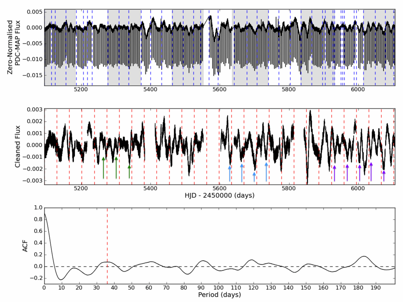
Figure 4: Upper panel. PDC-MAP LC light curve of Kepler-77, with the location of known instrumental systematic features marked by blue dashed lines. Grey and white bands denote the zero-normalised Q₃–Q₁₃ data. Middle panel. Cleaned and zero-normalised light curve, following subtraction of the best-fitting transit model. Rotational period intervals are shown with red dashed lines. The arrows mark groups (per colour) of repeated features. Lower panel. Autocorrelation function (ACF) of the cleaned and zero-normalised light curve. The red dashed line marks the peak corresponding to the 36-day rotational period of Kepler-77.

Although the PDC-MAP algorithm removes systematic instrumental fluctuations correlated across different stars in the same CCD channel, we cannot rule out residual instrumental effects and stochastic errors superimposed on the stellar variability (Figure 4, upper panel). A visual inspection of the raw and PDC-MAP data resulted in the identification of three regions of the light curve with anomalously high amplitude variability that does not look astrophysical in shape. These regions occupy the in HJD - 2 450 0000 time intervals between 5383 – 5413, 5563 – 5603, and 5813 – 5843 days (Figure 4, middle panel). They were masked when calculating the ACF to minimise the effect of residual systematics, and, like other gaps in the light curve, they were set to zero to prevent them contributing to the ACF. Q₁ and Q₂ were also excluded due to the short length of Q₁ and the considerable contamination by instrumental faults in Q₂.

The ACF of the cleaned, best-fit transit model-subtracted light curve displays correlation peaks at $\sim$17.5 and $\sim$36 days (Figure 4, lower panel). The latter is the dominant peak, and we attributed the peak at 17.5 days to a partial correlation between active regions at opposite longitudes of the star. To estimate the period and its error, we fitted a Gaussian function to the correlation peak and found $P_{\mathrm{rot}}=36\pm 6$ days. The projected rotational velocity $v$ sin $i_{\star}$ $=1.5\pm 1.0$  km s^-1 and the stellar radius $R_{\star}=0.99\pm 0.02$ $R_{\odot}$ give an upper limit on the rotational period of $33.4\pm 11.1$ days, which agrees with our $P_{\mathrm{rot}}$ estimate.

Repeated features visible in the light curve, such as those marked with the arrow sets in the middle panel of Figure 4, lead us to believe that the detected period results from spot modulation of the light curve.

5 Photometric and spectroscopic global analysis

We characterised the planet and its orbit via a simultaneous joint fit to the light curve and RV measurements using methods based on Bayesian statistics.

The Kepler photometric data included in the analysis is a subset of the whole light curve. We selected 12 hours of data-points around each transit and de-trended the individual transit light curves using a second-order polynomial fitted to the out-of-transit points. We preferred SC light curves when available, and excluded the LC transits for which SC data was available. The final SC and LC light curves contain $\sim$76800 and $\sim$4500 points, respectively.

We used a Bayesian approach for the parameter estimation, and sampled the parameter posterior distributions using Markov chain Monte Carlo (MCMC). The log-posterior probability was described as

$$\begin{split}\log P(\@vec{\theta}|D)=&\log P(\@vec{\theta})\\ &+\log P(V_{\mathrm{FIES}}|\@vec{\theta})+\log P(V_{\mathrm{Sand}}|\@vec{\theta})\\ &+\log P(F_{\mathrm{SC}}|\@vec{\theta})+\log P(F_{\mathrm{LC}}|\@vec{\theta})\,,\end{split}$$ (1)

where $V_{\mathrm{FIES}}$ and $V_{\mathrm{Sand}}$ correspond to the FIES and Sandiford radial velocity data, $F_{\mathrm{SC}}$ and $F_{\mathrm{LC}}$ are the short- and long-cadence photometric data, $\@vec{\theta}$ is the parameter vector, and $D$ the combined dataset. The first term in the right-hand side of Equation 1, namely $\log P(\@vec{\theta})$, represents the logarithm of the joint prior probability (the product of individual parameter prior probabilities), and the four remaining terms are the likelihoods for the radial velocity and light curve data. The likelihoods of the combined dataset $D$ follow the basic form for a likelihood assuming independent identically distributed errors following normal distribution:

$$\begin{split}\log P(D|\@vec{\theta})=&-\frac{N_{\mathrm{D}}}{2}\log(2\pi)-N_{\mathrm{D}}\log(\sigma_{\mathrm{D}})\\ &-\sum_{i=1}^{N_{\mathrm{D}}}\left(\frac{D_{i}-M(t_{i},\@vec{\theta})}{\sigma_{\mathrm{D}}}\right)^{2}\,,\end{split}$$ (2)

where $D_{i}$ is the single observed data point $i$, $M(t_{i},\@vec{\theta})$ the model explaining the data, $t_{i}$ the centre time for a data point $i$, $N_{\mathrm{D}}$ the number of data points and $\sigma_{\mathrm{D}}$ the standard deviation of the error distribution (a more detailed derivation can be found, e.g., in Gregory 2005).

The radial velocity model follows from equation

$$V=V_{\gamma}+K[\cos(\omega+\nu)+e\cos\omega]\,,$$ (3)

where $V_{\gamma}$ is the systemic velocity, $K$ the radial velocity semi-amplitude, $\omega$ the argument of periastron, $\nu$ the true anomaly, and $e$ the eccentricity. To account for the RV offset between Sandiford and FIES, we used two separate systemic velocities for the two different datasets, but did not consider linear (or higher order) velocity trends.

The transit model used our implementation of the transit-shape model described in Giménez (2006) and optimised for light curves with a large number of data points. The long-cadence model was super-sampled using ten subsamples per LC exposure to reduce the effects from the extended integration time, a necessity noted by Kipping (2010). The widening of the ingress and egress durations is clearly visible in the phase-folded long-cadence transit light curve plotted in Fig. 5 (right panel).

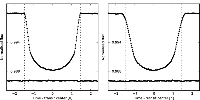
Figure 5: Phase-folded transit light curve of Kepler-77. Short- and long-cadence Kepler data are shown in the left and right panel, respectively, binned at $\sim$1.7 minutes. The best-fitting model is overplotted with a solid grey line. The dashed vertical lines mark the planet’s true first and fourth contact. The apparent transit duration is longer for the LC data than for the SC data, owing to the low time resolution.

The final joint model had 12 free parameters: orbital period $P_{\mathrm{orb}}$, the epoch of mid-transit $T_{\mathrm{c}}$, transit duration $T_{14}$, planet-to-star area ratio $R_{\mathrm{P}}^{2}/R_{\star}^{2}$, impact parameter $b=a_{\mathrm{P}}\,cos\,(i_{\mathrm{P}})/R_{\star}$, linear $u_{1}$ and quadratic $u_{2}$ limb-darkening coefficients, SC photometric scatter $\sigma_{\mathrm{SC}}$, LC photometric scatter $\sigma_{\mathrm{LC}}$, radial velocity semi-amplitude $K$, and two systemic velocities, i.e, one for Sandiford $V_{\gamma\,\mathrm{Sand}}$ and one for FIES $V_{\gamma\,\mathrm{FIES}}$. When fitting for a non-zero orbital eccentricity, two additional parameters were included, namely, the eccentricity $e$ and argument of periastron $\omega$.

We used uninformative priors (uniform) on all parameters. An initial fit for an eccentric orbit yielded $e=0.10^{+0.11}_{-0.07}$ and $\omega=104.6^{+72.8}_{-31.4}$ degrees. We note that the derived non-zero eccentricity is lower than a $2\,\sigma$ detection. Furthermore, the system parameters derived for an eccentric orbit are well within $1\,\sigma$ from those obtained for a circular solution. Following the F-test described in Lucy & Sweeney (1971), we found that there is a 66 % probability that the best-fitting eccentric solution could have arisen by chance if the orbit were actually circular. We thus decided to adopt a circular orbit ($e=0$). This assumption is also corroborated by the time-scale of orbital eccentricity dampening due to tidal interactions with the host star ($\tau_{e}=-e/\dot{e}$). Following the formalism of, e.g., Yoder & Peale (1981) and Matsumura et al. (2010), and assuming tidal dissipation quality factors $Q_{\mathrm{p}}\approx 10^{4}-10^{6}$ for gas giant planets (e.g., Carone 2012), we found that $\tau_{e}=-e/\dot{e}\leq 0.5$ Gyr, i.e., at least one order of magnitude younger than the age of the system ($7.5\pm 2.0$ Gyr). Moreover, the negative search for other companions in the system makes it unlikely that a perturber is continually stirring up the eccentricity of Kepler-77b (Sect. 6.3). We can thus safely assume that a hypothetical initial eccentric orbit of Kepler-77b has most likely been circularised by tides in the past.

We carried out the sampling of the posterior distribution with emcee (Foreman-Mackey et al. 2012), a Python implementation of the affine invariant Markov chain Monte Carlo sampler (Goodman & Weare 2010), which offers excellent sampling properties. The sampling was carried out using 500 walkers (chains). We first ran the sampler iteratively through a burn-in period consisting of 10 runs of 300 steps each, after which the walkers had converged to the posterior distribution. The final sample consists of 500 iterations with a thinning factor of 10, leading to 25 000 independent posterior samples. The affine invariant sampler is good at sampling correlated parameter spaces, and the fitting parameter set is designed to reduce the correlations (except when linear and quadratic limb-darkening coefficients are used directly instead of their linear combinations, as is usually done). We chose a thinning factor of 10 based on the parameter autocorrelation lengths to ensure that the samples can be considered to be independent.

The best-fitting system parameters were taken to be the median values of the posterior probability distributions. Error bars were defined at the 68 % confidence limit. We summarise our results in Table 6 and show the radial velocity and photometric data along with the best-fitting models in Figs.2 and 5, respectively.

6 Discussion and conclusion

6.1 Properties of the planet

With a mass of M_p $=0.430\pm 0.032$ $\mathrm{M}_{\mathrm{Jup}}$, radius of R_p $=0.960\pm 0.016$ $\mathrm{R}_{\mathrm{Jup}}$, and bulk density of $\rho_{\mathrm{p}}=0.603\pm 0.055$  g cm^-3, Kepler-77b joins the growing number of bloated gas-giant planets on a $\sim$3-day orbit. We used the empirical radius calibration for Saturn-mass planets found by Enoch et al. (2012) to estimate the predicted radius of Kepler-77b, given the planetary mass $M_{\mathrm{p}}$, equilibrium temperature $T_{\mathrm{eq}}$, semi-major axis $a_{\mathrm{p}}$, and stellar metallicity [M/H] (Table 6). Assuming a circular orbit - therefore omitting the contribution from tidal-dissipation - we found a predicted radius of $1.10\pm 0.13$ $\mathrm{R}_{\mathrm{Jup}}$, which agrees within $1\,\sigma$ with the measured values. Taking into account the relatively high metallicity of the star [M/H] $=0.20\pm 0.05$ dex, this further more proves that the radii of Saturn-mass planets ($\sim$0.1–0.5 $\mathrm{M}_{\mathrm{Jup}}$) are almost exclusively dependent on their mass and heavy-element content (see equation 7 in Enoch et al. 2012), with the second parameter affecting the mass of their cores (Guillot et al. 2006).

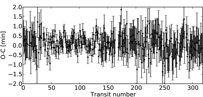
Figure 6: Differences between the observed and modelled transit centre times. The residuals show some structures, but they are only marginally significant.

6.2 Search for planet occultation: the albedo of Kepler-77b

The superb photometric quality of Kepler light curves allows one to detect secondary eclipses with very high accuracy and measure the planet albedo. Following the method described in Parviainen et al. (2013), we carried out a search for occultations of Kepler-77b by its host star. The search was performed at different orbital phases to allow for an eccentric orbit. Briefly, we modified the model used for the system characterisation to include the secondary eclipse - which was parameterised by the planet-to-star surface brightness ratio $f_{\mathrm{p}}/f_{\star}$ - and sampled the posterior distributions using emcee, as performed for the basic characterisation run of the system.

No significant occultation signals were identified. Based on the simulation results, we were able to set a 95 % confidence upper limit on the planet-to-star surface brightness ratio of $(f_{\mathrm{p}}/f_{\star})_{\mathrm{max}}$ = $0.001$, which is compatible with the photometric precision. Given the planet-to-star area ratio $R_{\mathrm{P}}^{2}/R_{\star}^{2}=0.009849\pm 0.000051$ (Table 6), this translates into an upper limit on the depth of the secondary eclipse of $\Delta I_{max}$=$(f_{\mathrm{p}}/f_{\star})_{\mathrm{max}}$ $R_{\mathrm{P}}^{2}/R_{\star}^{2}$$\approx$10 ppm.

The upper limit of the planet-to-star surface brightness ratio $(f_{\mathrm{p}}/f_{\star})_{\mathrm{max}}$ = $0.001$ allows us to constrain the upper limits of the geometric $A_{\mathrm{g}}$ and Bond $A_{\mathrm{B}}$ albedo of the planet. From the system parameters listed in Table 6, i.e., zero-eccentricity, effective stellar temperature $T_{\mathrm{eff}}$ $=5520\pm 60$ K, scaled semi-major axis $a_{\mathrm{p}}/R_{\star}=9.764\pm 0.055$, and assuming $A_{\mathrm{g}}=1.5\,A_{\mathrm{B}}$ and heat redistribution factor between 1/4 and 2/3, we found that $A_{\mathrm{g}}\leq 0.087\pm 0.008$ and $A_{\mathrm{B}}\leq 0.058\pm 0.006$. This makes Kepler-77b one of the gas-giant planets with the lowest albedo known to date, falling into range of albedos of TrES-2b (Kipping & Spiegel 2011) and HD 209458b (Rowe et al. 2008).

6.3 Search for additional planets

We performed a photometric search for additional planets in the Kepler-77 system.

Additional transits: We searched the photometric data for additional transiting companions in the system. For this purpose, we used the techniques of Ofir & Dreizler (2013) on all the publicly available Kepler data. We cleaned the light curve by removing all in-transit data points of Kepler-77b and remaining transient effects, and used the optimal box least-squares (BLS) algorithm (Ofir 2013) to search for additional transit signals. No additional transit signals were detected, in accordance with the trend that close-in giant planets do not tend to be found in transiting multi-planet systems (e.g., Batalha et al. 2013).

Transit-timing variation: Transits of a planets perturbed by additional objects are not strictly periodic. We carried out a search for dynamically induced deviations from a constant orbital period, i.e., we searched for variations in the transit centre times of Kepler-77b (transit-timing variations, TTVs). The search was carried out with an MCMC method similar to that used to characterise the planetary system (Sect 5). We expanded the light curve model to include each time of central transit as a free parameter, yielding a model with a total of 308 parameters. The parameter priors were based on the posterior densities of the basic characterisation run. We approximated the posteriors of the characterisation run parameters with a normal distribution and used uninformative uniform priors on the transit centre times. The sampling was carried out with emcee using 2000 parallel chains (walkers) and a notably longer burn-in phase.

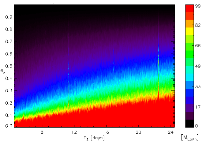
Figure 7: Maximum possible mass for a hypothetical perturber object in the Kepler-77 system as a function of its orbital period ($P_{2}$, in days) and eccentricity ($e_{2}$). Colours encode the upper limits of its mass (in Earth masses).

The result of our TTVs search is shown in Fig. 6, where the differences between the observed and modelled transit centre times - the so-called O$-$C diagram - are plotted against the transit number. We found that the transit centres do not deviate significantly from the linear ephemeris. The TTVs have a standard deviation of $\sim$0.5 minutes, with an absolute amplitude not exceeding $\sim$2 minutes. This value agrees with the result of Ford et al. (2011), who, based upon the Q₁ and Q₂ Kepler data, found a maximum absolute variation of $\sim$1.8 minutes for Kepler-77b.

The lack of detectable TTVs in the Q₁–Q₁₃ Kepler light curve can be used to exclude certain types of companions. We used the approach described in Csizmadia et al. (2010) to give upper limits on the mass of a hypothetical perturbing object. Thirty thousand independent values of its orbital period and eccentricity were randomly chosen. Using the formalism of Agol et al. (2005), at each given period and eccentricity, we calculated the perturber’s maximum allowable mass that would cause TTV-amplitude shorter than 0.5 minutes (i.e., $1\,\sigma$). This formalism takes only coplanar orbits into account. Any mass-period-eccentricity combination that would cause a larger TTV-amplitude in the observational window considered in this paper ($\sim$3 years) can be excluded. The upper limits for the hypothetical perturber in a coplanar orbit are shown in Fig. 7 as a function of its orbital period ($P_{2}$) and eccentricity ($e_{2}$). If there were a perturber on a short-period ($P_{2}\lessapprox 24$ days) and low-eccentricity ($e_{2}\lessapprox 0.1$) orbit, it probably has a mass smaller than $\sim$100 M_Earth. Low-mass ($M_{2}\leq 17$ M_Earth) planets on highly eccentric ($e_{2}\geq 0.3$) coplanar orbits cannot be ruled out with the currently available photometry. The possible existence of such planets should be studied in more details by stability investigations, which is beyond the scope of the present paper.

Planetary systems hosting hot-Jupiters are frequently considered as single-planet systems because no additional sub-stellar companions are detected, with only a handful of them showing TTVs (e.g., Szabó et al. 2012). Short time-scale TTVs are rarely present in systems harbouring close-in giant planets, and Kepler-77 agrees with this trend. A remarkable exception is WASP-12b (Maciejewski et al. 2013). The observed TTVs in some other systems hosting hot-Jupiters are often due to systematic observational effects (Szabó et al. 2012), stellar activity (Barros et al. 2013), and small-number statistics (Fulton et al. 2011; Southworth et al. 2012), rather than gravitational perturbations.

6.4 Search for spot-crossing events: constraints on the spin-orbit obliquity

Occultations of active photospheric regions by transiting planets can be used to constrain the spin-orbit obliquity of planetary systems (see, e.g., Nutzman et al. 2011; Sanchis-Ojeda et al. 2011, 2012), i.e., the angle between the stellar spin axis and the angular momentum vector of the orbit. The spin-orbit obliquity of planetary systems hosting close-in ($a\lessapprox 0.15$ AU) gas giant planets is considered a keystone to investigate their formation, migration, and subsequent tidal interaction (see, e.g., Winn et al. 2010; Morton & Johnson 2011; Gandolfi et al. 2012).

We searched for photometric anomalies in the transit light curves of Kepler-77 resulting from the passage of the planet in front of Sun-like spots. The search was carried out by removing the best-fitting transit signal from the 106 SC transit light curves and looking for systematic features in the residuals. The search was performed two-dimensionally by looking for features occurring during individual transits (planet crossing over a single feature) and over multiple transits (planet crossing over the same, possibly changing, feature over multiple transits).

No significant anomalies were identified above the noise level (1398 ppm $\approx$ 1.5 mmag) in the $\sim$1.2-year time window covered by the SC data, as shown in Fig. 8. The transits show marginal variations in the overall depth, which could be attributed to different levels of spot-coverage in the non-transited parts of the visible stellar disk, as suggested by the out-of-transit modulation visible in the light curve of Kepler-77 (Fig. 1).

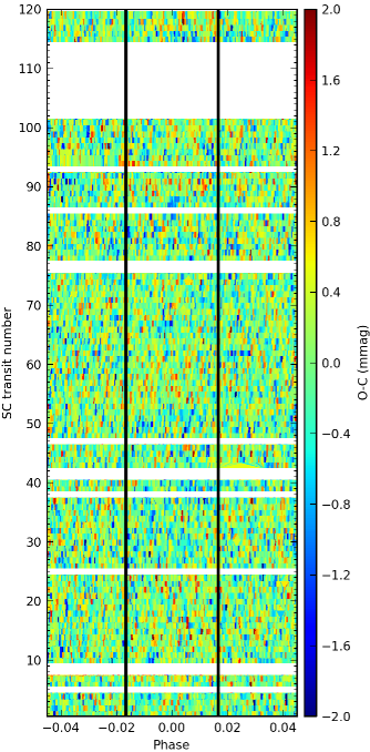
Figure 8: Short-cadence transit residuals map of Kepler-77, following the subtraction of the best-fitting transit model. Orbital phase increases from left to right, SC transit number from bottom to top. The two vertical thick lines mark the transit first and fourth planet’s contact. The white bands, as well as the diagonal features in the residual map are caused by the lack of Kepler photometric data.

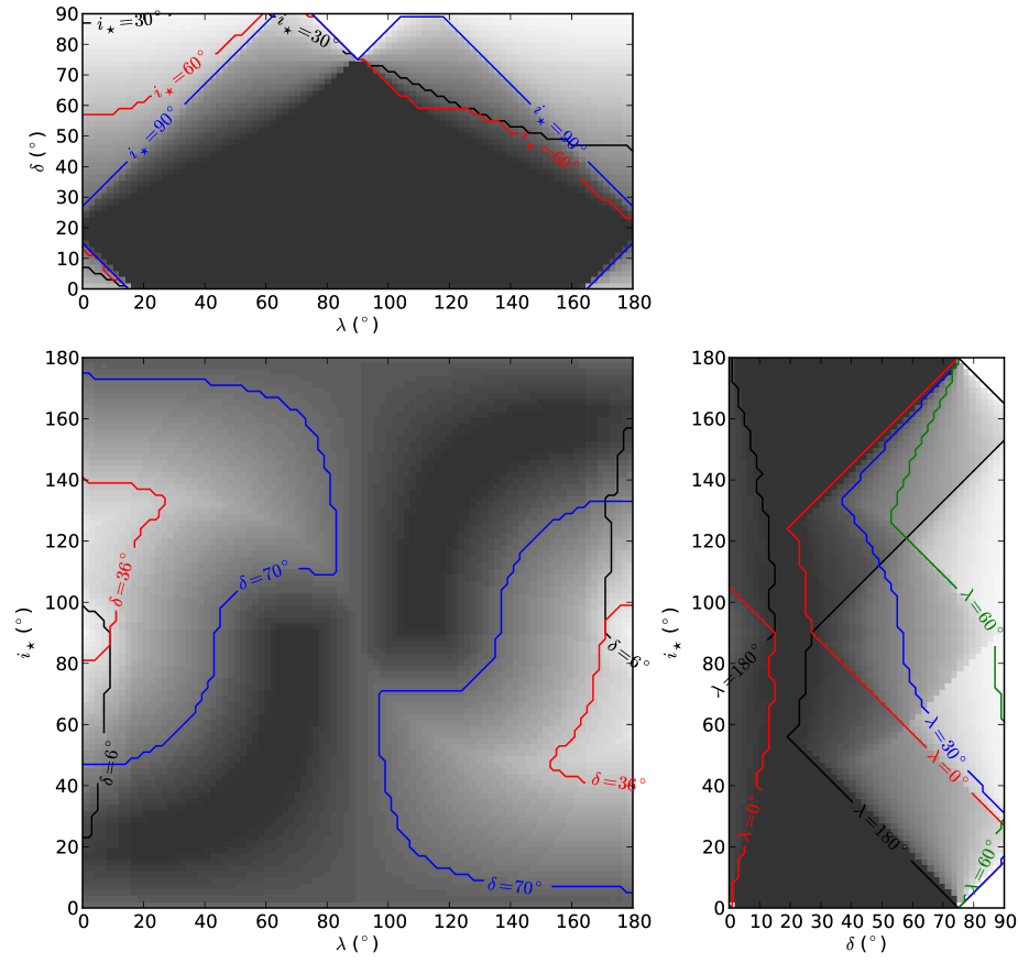
Figure 9: Two-dimensional projections of the joint probability distribution for the stellar inclination $i_{\star}$, the characteristic latitude of active regions $\delta$, and the sky-projected spin-orbit angle $\lambda$ (see text for details).

The effective temperature of spots in mid G-type stars is estimated to be $\sim$1500 K cooler than the unperturbed photosphere (see, e.g., Strassmeier 2009). With a SC photometric precision of 1398 ppm, we can safely exclude occultations of starspots whose radius is larger than $\sim$0.04 stellar radii (assuming circular shape and neglecting limb-darkening, geometrical foreshortening, and penumbra/umbra effects). The $\sim$0.4 % out-of-transit stellar variability (Fig. 1) indicates the presence of spots with a radius of $\sim$0.08 stellar radii. This suggests that the non-detection of significant anomalies is rather due to the non-intersection between the transit chord and the active latitudes of the star, and not to the lack of photometric precision.

In the Sun active regions tend to emerge predominantly at specific latitudes, which are symmetrically placed with respect to the solar equator. Over the course of the Sun’s 11-year activity cycle, active latitudes gradually migrate from the mid-latitude (about $\pm 35\hbox{${}^{\circ}$}$) towards the equator (about $\pm 5\hbox{${}^{\circ}$}$), giving rise to the well-known butterfly diagram (see, e.g., Li et al. 2001). The spectral type, age, and photometric modulation of Kepler-77 are fairly similar to those of the Sun. It therefore seems reasonable to assume that photospheric active regions in Kepler-77 also fall primarily within two latitude bands that are symmetric with respect to the stellar equator. If we assume that spots on Kepler-77 were also confined to a given active latitude during the $\sim$1.2 years observations analysed here, then we can use the absence of spot-crossing events to place a joint constraint on the stellar inclination $i_{\star}$, the sky-projected spin-orbit obliquity $\lambda$, and the characteristic absolute latitude of the spots $\delta$.

To map out the region of $(i_{\star},\lambda,\delta)$-space that is excluded by the lack of detected spot crossings, we tracked a hypothetical point-like spot with latitude $\delta$ as the star rotates, and checked whether it overlapped with the transit chord at any point. If so, the particular combination of $i_{\star}$, $\lambda$, and $\delta$ was considered ruled out. We then repeated the process over a grid of values ranging from $0$ to $180\hbox{${}^{\circ}$}$ for $i_{\star}$ and $\lambda$, and from $0$ to $90\hbox{${}^{\circ}$}$ for $\delta$. Details of the calculation are given in Appendix A. Note that considering this domain only does not imply any loss of generality; we are effectively assuming that if there are spots at $+\delta$, there are also spots at $-\delta$, and acknowledging that we are only sensitive to $i_{\star}\,\mathrm{mod}\,180\hbox{${}^{\circ}$}$ and to $|\lambda|$ (i.e., $i_{\star}$ and $i_{\star}+180\hbox{${}^{\circ}$}$ are indistinguishable, as are $\lambda$ and $-\lambda$). Note also that we imposed no constraints on the stellar inclination $i_{\star}$, as the large relative error of the projected rotational velocity ($v$ sin $i_{\star}$ $=1.5\pm 1.0$  km s^-1) does not allow us to make a meaningful measurement of $i_{\star}$.

Figure 9 shows the two-dimensional projections of the three-dimensional grid; lighter regions mean that most combinations of the quantities along the $x$- and $y$-axis are permitted, and darker regions mean that most such combinations are excluded. The contours mark the edges of the permitted/excluded regions for specific values of the third angle. The predominantly grey area surrounded by blue contour in the upper left panel of Figure 9 shows the region of the $(\lambda,\delta)$-space that is excluded by the absence of spot-crossing event during the transits if the star is seen equator on. As the contours show, this region changes only slowly as the stellar inclination decreases, i.e., the constraints remain more or less unchanged if the star is seen close to, but not exactly equator-on. If active regions in Kepler-77 appeared within the same absolute latitude range observed in the Sun ($\sim$5–35^∘), for any value of the stellar inclination $i_{\star}$, the lack of starspots occultations in the transit light curve of Kepler-77 would imply $|\lambda|\lessapprox 26\hbox{${}^{\circ}$}$ or $154\hbox{${}^{\circ}$}\lessapprox\lambda\lessapprox 206\hbox{${}^{\circ}$}$ (Figure 9, middle left panel).

The SC Kepler data available at the time of writing cover $\sim$1.2 years. If Kepler-77 possesses an activity cycle similar to the Sun’s, during which its active regions migrate in latitude, then starspots might drift into the range where they overlap with the transit chord over the next few years. Occultations of starspots by the planet would then become visible during its transits. This would allow us to study the magnetic cycle of the star and put stronger constraints on the spin-orbit obliquity of the system.

Table 3: Kepler-77 system parameters.

Model parameters
Planet orbital period $P_{\mathrm{orb}}$ [days]	$3.57878087\pm 0.00000023$
Planetary transit epoch $T_{\mathrm{c}}$ [HJD-2 450 000]	$5095.865727\pm 0.000029$
Planetary transit duration $T_{14}$ [days]	$0.12224\pm 0.00014$
Planet-to-star area ratio $R_{\mathrm{p}}^{2}/R_{\star}^{2}$	$0.009849\pm 0.000051$
Impact parameter $b$	$0.341\pm 0.017$
Linear limb-darkening coefficient $u_{1}$	$0.505\pm 0.015$
Quadratic limb-darkening coefficient $u_{2}$	$0.139\pm 0.032$
Kepler LC data scatter $\sigma_{\mathrm{LC}}$ [ppm]	$378.1\pm 3.8$
Kepler SC cadence data $\sigma_{\mathrm{SC}}$ [ppm]	$1397.5\pm 3.6$
Radial velocity semi-amplitude $K$ [ m s-1]	$59.2\pm 4.3$
Systemic velocity (Sandiford) $V_{\gamma\,\mathrm{Sand}}$ [ km s-1]	$-24.7843\pm 0.0120$
Systemic velocity (FIES) $V_{\gamma\,\mathrm{FIES}}$ [ km s-1]	$-24.7567\pm 0.0035$
Derived parameters
Planet-to-star radius ratio $R_{\mathrm{p}}/R_{\star}$	$0.09924\pm 0.00026$
Scaled semi-major axis of the planetary orbit $a_{\mathrm{p}}/R_{\star}$	$9.764\pm 0.055$
Semi-major axis of the planetary orbit $a_{\mathrm{p}}$ [AU]	$0.04501\pm 0.00063$
Orbital inclination angle $i_{\mathrm{p}}$ [degree]	$88.00\pm 0.11$
Orbital eccentricity $e$	0 (fixed)
Ingress – egress duration $T_{12}=T_{34}$	$0.02478\pm 0.00036$
Bulk stellar density $\rho_{\star}$ [ g cm-3]	$1.365\pm 0.023$
Stellar fundamental parameters
Effective temperature $T_{\mathrm{eff}}$ [K]	$5520\pm 60$
Surface gravity log $g$ [dex]	$4.40\pm 0.10$
Surface gravity log $g$ [dex]	$4.42\pm 0.01$
Metallicity $[\mathrm{M/H}]$ [dex]	$0.20\pm 0.05$
Microturbulent velocity $v_{\mathrm{micro}}$ [ km s-1]	$0.9\pm 0.1$
Macroturbulent velocity $v_{\mathrm{macro}}$ [ km s-1]	$1.8\pm 0.3$
Projected stellar rotational velocity $v$ sin $i_{\star}$ [ km s-1]	$1.5\pm 1.0$
Spectral type	G5 V
Star mass $M_{\star}$ [$M_{\odot}$]	$0.95\pm 0.04$
Star radius $R_{\star}$ [$R_{\odot}$]	$0.99\pm 0.02$
Star age $t$ [Gyr]	$7.5\pm 2.0$
Star rotation period $P_{\mathrm{rot}}$ [days]	$36\pm 6$
Interstellar extinction $A_{\mathrm{V}}$ [mag]	$0.08\pm 0.04$
Distance of the system $d$ [pc]	$570\pm 70$
Planetary fundamental parameters
Planet mass $M_{\mathrm{p}}$ [$\mathrm{M}_{\mathrm{Jup}}$]	$0.430\pm 0.032$
Planet radius $R_{\mathrm{p}}$ [$\mathrm{R}_{\mathrm{Jup}}$]	$0.960\pm 0.016$
Planet density $\rho_{\mathrm{p}}$ [ g cm-3]	$0.603\pm 0.055$
Equilibrium temperature $T_{\mathrm{eq}}$ [K]	$1440^{+100}_{-120}$
Geometric albedo $A_{\mathrm{g}}$	$\leq 0.087\pm 0.008$
Bond albedo $A_{\mathrm{B}}$	$\leq 0.058\pm 0.006$

Appendix A Tracking a rotating starspot with respect to the transit chord

The geometry of the system is shown in Figure 10. We started by considering a right-handed reference frame $S$, whose origin coincides with the centre of the star. In this frame, the stellar rotation vector defines the $+z$-direction, while the $y$-axis lies in the plane of the sky. If we set the stellar radius to unity, the coordinates of a starspot with latitude $\delta$ in this reference frame are simply

$$\left[\begin{array}[]{l}x\\ y\\ z\end{array}\right]=\left[\begin{array}[]{l}\cos\delta\cos\phi\\ \cos\delta\sin\phi\\ \sin\delta\end{array}\right]\,,$$

where $\phi=2\pi t/P_{\mathrm{rot}}+\phi_{0}$, $P_{\mathrm{rot}}$ is the star’s rotational period, and $\phi_{0}$ is the longitude of the spot at some arbitrary time $t=0$.

We defined a second right-handed reference frame $S^{\prime}$ that shares the same origin and $y$-axis as frame $S$ (i.e., $y^{\prime}\equiv y$), but whose $x^{\prime}$-axis is pointing towards the observer. The stellar inclination $i_{\star}$ is the angle between the stellar rotation axis and the line-of-sight, i.e., the angle in the $x^{\prime}z^{\prime}$-plane between the $z$-axis of frame $S$ and the $x^{\prime}$-axis of frame $S^{\prime}$. Coordinates in frame $S$ are transformed to frame $S^{\prime}$ by performing a rotation by $-(\pi/2-i_{\star})$ about the $y$-axis (or, equivalently, around the $y^{\prime}$-axis; see Figure 10, left panel). This process is described in more detail in Appendix A of Aigrain et al. (2012).

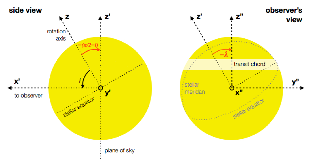
Figure 10: System geometry seen from the side (left) and from the observer’s standpoint (right), illustrating the two rotations needed to convert from frame $S$ to frame $S^{\prime\prime}$ (see text for details).

We then considered a third right-handed reference frame $S^{\prime\prime}$ that shares the same origin as $S$ and $S^{\prime}$, and the same $x$-axis as frame $S^{\prime}$ (i.e., $x^{\prime\prime}\equiv x^{\prime}$), but has its $y^{\prime\prime}$-axis parallel to the transit chord. The sky-projected spin-orbit angle $\lambda$ is defined as the angle in the plane of the sky between the projections of the orbital angular momentum and of the stellar spin axis, i.e., the angle in the $y^{\prime\prime}z^{\prime\prime}$-plane between the $z^{\prime\prime}$-axis of frame $S^{\prime\prime}$ and the $z^{\prime}$-axis of frame $S^{\prime}$. Coordinates in frame $S^{\prime}$ are transformed to frame $S^{\prime\prime}$ by performing a second rotation by $-\lambda$ about the $x^{\prime}$-axis (or, equivalently, around the $x^{\prime\prime}$-axis; see Figure 10, right panel). The coordinates of the spot in frame $S^{\prime\prime}$ are thus

$$\centering\begin{array}[]{rcl}\left[\begin{array}[]{l}x^{\prime\prime}\\ y^{\prime\prime}\\ z^{\prime\prime}\end{array}\right]&=&\left[\begin{array}[]{l}\cos\delta\cos\phi\sin i_{\star}+\sin\delta\cos i_{\star}\\ \cos\lambda\cos\delta\sin\phi+\sin\lambda\cos\delta\cos\phi\cos i_{\star}-\sin\lambda\sin\delta\sin i_{\star}\\ \sin\lambda\cos\delta\sin\phi-\cos\lambda\cos\delta\cos\phi\cos i_{\star}+\cos\lambda\sin\delta\sin i_{\star}.\end{array}\right].\end{array}\@add@centering$$

If we observe the system for an infinite amount of time, a given spot that remains static relative to the rotating surface of the star will eventually be crossed by the planet during a transit, if, and only if,

$$x^{\prime\prime}>0\leavevmode\nobreak\ {\rm and}\leavevmode\nobreak\ b-R_{\mathrm{p}}/R_{\star}<z^{\prime\prime}<b+R_{\mathrm{p}}/R_{\star}.$$

The absence of spot crossings therefore excludes a specific volume in $(i_{\star},\lambda,\delta)$-space that we explored by following the variations of $x^{\prime\prime}$ and $z^{\prime\prime}$ as $\phi$ varies. In the present study, this was done by stepping through a grid of values, ranging from $0$ to $180\hbox{${}^{\circ}$}$ for $i_{\star}$ and $\lambda$, and from $0$ to $90\hbox{${}^{\circ}$}$ for $\delta$, with $2\hbox{${}^{\circ}$}$ steps. At each point of the grid, $x^{\prime\prime}$ and $z^{\prime\prime}$ were evaluated over a grid of $\phi$-values, ranging from $0$ to $360\hbox{${}^{\circ}$}$ with $2\hbox{${}^{\circ}$}$ steps. If the conditions above (evaluated using the values for $b$ and $R_{\mathrm{p}}/R_{\star}$ given in Table 6, i.e., 0.341 and 0.09924, respectively) were met for any value of $\phi$, the corresponding cell in the $(i_{\star},\lambda,\delta)$ grid was considered excluded.

References

- Adams et al. (2012) Adams, E. R., Ciardi, D. R., Dupree, A. K., et al. 2012, AJ, 144, 42
- Agol et al. (2005) Agol, E., Steffen, J., Sari, R. & Clarkson, W. 2005, MNRAS, 359, 567
- Aigrain et al. (2012) Aigrain, S., Pont, F., Zucker, S. 2012, MNRAS, 419, 3147
- Alonso et al. (2012) Alonso, R., Guenther, E. W., Almenara, J.-M., et al. 2012, A&A, submitted
- Baglin et al. (2006) Baglin, A., Auvergne, M., Boisnard, L., et al. 2006, 36th COSPAR Scientific Assembly, 36, 3749
- Barclay et al. (2013) Barclay, T., Rowe, J F., Lissauer, J. J., et al. 2013, Nature, 494, 452
- Barnes & Kim (2010) Barnes, S. A. & Kim, Y.-C. 2010, ApJ, 721, 675
- Barnes (2010) Barnes, S. A. 2010, ApJ, 722, 222
- Barros et al. (2013) Barros, S. C. C., Boué, G., Gibson, N. P., et al. 2013, MNRAS, 430, 3032
- Batalha et al. (2011) Batalha, N. M., Borucki, W.J̇., Bryson, S. T., et al. 2011, ApJ, 729, 27
- Batalha et al. (2013) Batalha, N. M., Rowe, J. F., Bryson, S. T., et al. 2013, ApJS, 204, 24
- Borucki et al. (2010) Borucki, W. J., Koch, D., Basri, G., et al. 2010, Science, 327, 977
- Borucki et al. (2010) Borucki, W. J., Koch, D., Basri, G., et al. 2011, ApJ, 728, 117
- Borucki et al. (2012) Borucki, W. J., Koch, D. G, Batalha, N., et al. 2012, ApJ, 745, 120
- Brown (2003) Brown, T. M. 2003, ApJ, 593, L125
- Bruntt et al. (2010) Bruntt, H., Bedding, T. R., Quirion, P.-O., et al. 2010, MNRAS, 405, 1907
- Buchhave et al. (2010) Buchhave, L. A., Bakos, G. A., Hartman, J. D., et al. 2010, ApJ, 720, 1118
- Carone (2012) Carone L. 2012, in “Tidal interactions of short-period extrasolar transit planets with their host stars: Constraining the elusive stellar tidal dissipation factor”, PhD thesis available at kups.ub.uni-koeln.de/4757/
- Casagrande (2007) Casagrande, L. 2007, ASPC, 374, 71
- Castelli & Kurucz (2004) Castelli, F. & Kurucz, R.L. 2004, eprint arXiv:astro-ph/0405087
- Coelho et al. (2005) Coelho, P., Barbuy, B., Meléndez, J., et al. 2005, A&A, 443, 735
- Colón et al. (2012) Colón, K. D., Ford, E. B., Morehead, R. C. et al. 2012, MNRAS, 426, 342
- Csizmadia et al. (2010) Csizmadia, Sz., Renner, S., Barge, P., et al. 2010, A&A, 510, A94
- Cutri et al. (2003) Cutri, R. M., Skrutskie, M. F., van Dyk, S., et al. 2003, in “2MASS All-Sky Catalog of Point Sources”, NASA/IPAC Infrared Science Archive
- Cyburt (2004) Cyburt, R. H., 2004, PhRvD, 70, 023505
- Deeg et al. (2010) Deeg, H. J., Moutou, C., Erikson, A., et al. 2010, Nature, 464, 384
- Degl’Innocenti et al. (2008) Degl’Innocenti, S., Prada Moroni, P. G., Marconi, M., Ruoppo, A. 2008, Ap&SS, 316, 25
- Dell’Omodarme et al. (2012) Dell’Omodarme, M., Valle, G., Degl’Innocenti, S., Prada Moroni, P. G. 2012, A&A, 540, A26
- Doyle et al. (2011) Doyle, L. R., Carter, J. A., Fabrycky, D. C., et al. 2011, Science, 333, 1602
- Enoch et al. (2012) Enoch, B., Collier Cameron, A. & Horne, K. 2012, A&A, 540, A99
- Ford et al. (2011) Ford, E. B., Rowe, J. F., Fabrycky, D. C., et al. 2011, ApJS, 197, 2
- Foreman-Mackey et al. (2012) Foreman-Mackey, D., Hogg, D W., Lang, D., et al. 2013, PASP, 125, 306
- Frandsen & Lindberg (1999) Frandsen, S. & Lindberg, B. 1999, in “Astrophysics with the NOT”, proceedings Eds: Karttunen, H. & Piirola, V., anot. conf, 71
- Frasca et al. (2003) Frasca, A., Alcalá, J. M., Covino, E., et al. 2003, A&A, 405, 149
- Frasca et al. (2006) Frasca, A., Guillot, P., Marilli, E., et al. 2006, A&A, 454, 301
- Fridlund et al. (2010) Fridlund, M., Hébrard, G., Alonso, R., et al. 2010, A&A, 512, A14
- Fulton et al. (2011) Fulton, B. J., Shporer, A., Winn, J. N., et al. 2011, AJ, 142, 84
- Gandolfi et al. (2008) Gandolfi, D., Alcalá, J. M., Leccia, S., et al. 2008, ApJ, 687, 1303
- Gandolfi et al. (2010) Gandolfi, D., Hébrard, G., Alonso, R., et al. 2010, A&A, 524, A55
- Gandolfi et al. (2012) Gandolfi, D., Collier Cameron, A., Endl, M., et al. 2012, A&A, 543, L5
- Gennaro et al. (2010) Gennaro, M., Prada Moroni, P. G. & Degl’Innocenti, S. 2010, A&A, 518, A13
- Giménez (2006) Giménez, A. 2006, A&A, 450, 1231
- Goodman & Weare (2010) Goodman, J. & Weare, J. 2010, Communications in Applied Mathematics and Computational Science, 5, 65
- Gregory (2005) Gregory, P. C. 2005, in “Bayesian Logical Data Analysis for the Physical Sciences: A Comparative Approach with ‘Mathematica’ Support”, Cambridge University Press
- Guillot et al. (2006) Guillot, T., Santos, N. C., Pont, F., et al. 2006, A&A, 453, L21
- Gustafsson et al. (2008) Gustafsson, B., Edvardsson, B., Eriksson, K., et al. 2008, A&A, 486, 951
- Hauschildt et al. (1999) Hauschildt, P. H., Allard, F. & Baron, E. 1999, ApJ, 512, 377
- Howell et al. (2011) Howell, S. B., Everett, M. E., Sherry, W., et al. 2011, AJ, 142, 19
- Jimenez et al. (2003) Jimenez, R., Flynn, C., MacDonald, J., et al. 2003, Science, 299, 1552
- Kipping (2010) Kipping, D. M. 2010, MNRAS, 408, 1758
- Kipping & Spiegel (2011) Kipping, D. M. & Spiegel, D. S. 2011, MNRAS, 417, L88
- Leger et al. (2009) Léger, A., Rouan, D., Schneider, J., et al. 2009, A&A, 506, 287
- Li et al. (2001) Li, K. J., Yun, H. S. & Gu, X. M. 2001, AJ, 122, 2115
- Lillo-Box et al. (2012) Lillo-Box, J., Barrado, D. & Bouy, H. 2012, A&A, 546, A10
- Lissauer et al. (2011) Lissauer, J., Fabricky, D., Ford, E. et al., 2011, Nature, 470, 53
- Lucy & Sweeney (1971) Lucy, L. B. & Sweeney, M. A. 1971, AJ, 76, 544
- Maciejewski et al. (2013) Maciejewski, G., Dimitrov, D., Seeliger, M., et al. 2013, A&A, 551, A108
- Matsumura et al. (2010) Matsumura, S., Peale, S. J. & Rasio F. A. 2010, ApJ, 725, 1995
- McCarthy et al. (1993) McCarthy, J. K., Sandiford, B. A., Boyd, D., Booth, J. 1993, PASP, 105, 881
- McQuillan et al. (2013) McQuillan, A., Aigrain, S., Mazeh, T. 2013, MNRAS, 432, 1203
- Morton & Johnson (2011) Morton, T. D. & Johnson, J. A. 2011, ApJ, 729, 138
- Morton & Johnson (2011) Morton, T. D. & Johnson, J. A. 2011, ApJ, 738, 170
- Nutzman et al. (2011) Nutzman, P. A., Fabrycky, D. C. & Fortney, J. J. 2011, ApJ, 740, L10
- Ofir & Dreizler (2013) Ofir, A. & Dreizler, S. 2013, A&A, 555, A58
- Ofir (2013) Ofir, A. 2013, in “Optimizing the search for transiting planets in long time series”, A&A, submitted
- Orosz et al. (2012) Orosz, J. A., Welsh, W. F., Carter, J. A., et al. 2012, Science, 337, 1511
- Parviainen et al. (2013) Parviainen, H., Deeg, H. J. & Belmonte, J. A. 2013, A&A, 550, A67
- Peimbert et al. (2007a) Peimbert, M., Luridiana, V., Peimbert, A., Carigi, L. 2007a, ASPC, 374, 81
- Peimbert et al. (2007b) Peimbert, M, Luridiana, V. & Peimbert, A. 2007b, ApJ, 666, 636
- Prugniel & Soubiran (2001) Prugniel, Ph. & Soubiran, C. 2001, A&A, 369, 1048
- Queloz et al. (2001) Queloz, D., Henry, G. W., Sivan, J. P., et al. 2001, A&A, 379, 279
- Rowe et al. (2008) Rowe, J. F., Matthews, J. M., Seager, S., et al. 2008, ApJ, 689, 1345
- Sanchis-Ojeda et al. (2011) Sanchis-Ojeda, R., Winn, J. N., Holman, M. J., et al. 2011, ApJ, 733, 127
- Sanchis-Ojeda et al. (2012) Sanchis-Ojeda, R., Fabrycky, D. C.; Winn, J. N., et al., 2012, Nature, 487, 449
- Santerne et al. (2012) Santerne, A., Díaz, R. F., Moutou, C., et al. 2012, A&A, 545, A76
- Smith et al. (2012) Smith, J. C., Stumpe, M. C., Van Cleve, J. E., et al. 2012, PASP, 124, 1000
- Southworth et al. (2012) Southworth, J., Bruni, I., Mancini, L., et al. 2012, MNRAS, 420, 2580
- Strassmeier (2009) Strassmeier, K. G. 2009, A&ARv, 17, 251
- Stumpe et al. (2012) Stumpe, M. C., Smith, J. C., Van Cleve, J. E., et al. 2012, PASP, 124, 985
- Szabó et al. (2012) Szabó, R., Szabó, Gy. M., Dálya, G., et al. 2013, A&A, 553, A17
- Thoul et al. (1994) Thoul, A. A., Bahcall, J. N. & Loeb, A. 1994, ApJ421, 828
- Tognelli et al. (2011) Tognelli, E., Prada Moroni, P. G. & Degl’Innocenti, S. 2011, A&A, 533, A109
- Udry et al. (1999) Udry, S., Mayor, M., Queloz, D. 1999, ASPC, 185, 367
- Valenti & Piskunov (1996) Valenti, J. A. & Piskunov, N. 1996, A&AS, 118, 595
- Valenti & Fischer (2005) Valenti, J. A. & Fischer, D. A. 2005, ApJS, 159, 141
- Winn et al. (2010) Winn, J. N., Fabrycky, D. C., Albrecht, S., et al. 2010, ApJ, 718, L145
- Wright et al. (2010) Wright, E. L., Eisenhardt, P. R. M., Mainzer, A. K., et al. 2010, AJ, 140, 1868
- Yoder & Peale (1981) Yoder, C. F. & Peale, S. J. 1981, Icarus, 47, 1