Joint Model-Order and Step-Size Adaptation using Convex Combinations of Adaptive Reduced-Rank Filters

Abstract

In this work we propose schemes for joint model-order and step-size adaptation of reduced-rank adaptive filters. The proposed schemes employ reduced-rank adaptive filters in parallel operating with different orders and step sizes, which are exploited by convex combination strategies. The reduced-rank adaptive filters used in the proposed schemes are based on a joint and iterative decimation and interpolation (JIDF) method recently proposed. The unique feature of the JIDF method is that it can substantially reduce the number of coefficients for adaptation, thereby making feasible the use of multiple reduced-rank filters in parallel. We investigate the performance of the proposed schemes in an interference suppression application for CDMA systems. Simulation results show that the proposed schemes can significantly improve the performance of the existing reduced-rank adaptive filters based on the JIDF method.

I Introduction

In the literature of adaptive filtering algorithms [1], numerous algorithms with different trade-offs between performance and complexity have been reported in the last decades. A designer can choose from the simple and low-complexity least-mean squares (LMS) algorithms to the fast converging though complex recursive least squares (RLS) techniques [1]. A great deal of research has been devoted to developing cost-effective adaptive filters with an attractive trade-off between performance and complexity and automatic tuning of key parameters [1]. Combination schemes [2]-[3] are recent and effective design approaches, where several filters are mixed in order to obtain an overall quality improvement. The individual filters are set up so as to optimize different desirable properties: fast tracking or low error in steady-state, for example. The combined filter is able to keep the advantages of all the individual filters, achieving superior performance despite a higher computational cost than the single filter approach. The computational complexity required by combination schemes is due to the use of two or more adaptive filters in parallel and can become unacceptably high with large filters [2]-[3].

Reduced-rank adaptive filters [4]-[10] are cost-effective techniques when dealing with problems involving large filters and reduced training. A number of reduced-rank adaptive filtering methods have been proposed in the last several years [4]-[10]. Among them are eigen-decomposition-based techniques [4], the multistage Wiener filter (MSWF) [5], the auxiliary vector filtering (AVF) algorithm [6], the interpolated reduced-rank filters [7], the reduced-rank filters based on joint and iterative optimization (JIO) [9] and joint iterative interpolation, decimation, and filtering (JIDF) [10]. Key problems with previously reported reduced-rank adaptive filters are the tuning of the step sizes and/or the forgetting factors, and the model-order selection [4]-[11].

In this paper, we propose schemes for joint model-order and step-size adaptation of reduced-rank adaptive filters based on the JIDF technique [10] which address these drawbacks of the JIDF scheme. The proposed schemes employ reduced-rank adaptive filters in parallel operating with different orders and step sizes, which are exploited by convex combination strategies. The main reason for choosing the JIDF technique [10] is that it allows a substantial reduction in the number of coefficients for adaptation and yields the best performance among the techniques reported so far. Although the number of coefficients that are actually adapted is smaller, leading to better convergence rates and mean-square error, the complexity of the JIDF is comparable to that of the full-rank LMS. Other reduced-rank schemes have in general a higher complexity. We derive least-mean squares (LMS) reduced-rank filters based on the JIDF method and propose strategies to automatically adjust the model-order and step sizes used. Without an interpolator, the JIDF approach may also address the main drawback of combination schemes, i.e., the increase in the number of elements for computation, but this possibility will be pursued elsewhere.

This paper is organized as follows. Section II presents the proposed convex combination schemes of reduced-rank adaptive filters. Section III is devoted to the derivation of the convex combiners and Section IV to the derivation of LMS algorithms with the JIDF approach. Section V presents and discusses the simulation results and Section VI draws the conclusions of this work.

II Proposed Combination Schemes

In this section, we detail the proposed convex combination schemes of reduced-rank adaptive filters. The basic idea behind these schemes is to employ a number of parallel sets of transformation matrices and reduced-rank filters that are jointly optimized and exploit them via the setting of different model orders and step sizes. The different model orders and step sizes are determined a priori. Since we are interested in this work in adapting the model order and the step size, then in principle we need at most $4$ parallel structures for setting upper and lower values for the model order (or rank) and the step sizes. To this end, we can build a tree structure where only two structures are combined at each stage. A block diagram of the first tree structured scheme, denoted scheme A, is shown in Fig. LABEL:fig1.

Let us now mathematically describe the signal processing performed by the proposed scheme A. Consider an $M\times 1$ input data vector ${\boldsymbol{r}}[i]$ that is processed by reduced-rank schemes in parallel with different parameters, namely the model order and the step size. The output of scheme A is given by

$$\begin{split}y_{c}[i]&=\lambda_{c}[i]y_{a}[i]+(1-\lambda_{c}[i])y_{b}[i]\\ &=\lambda_{c}[i]\Bigl{(}\lambda_{a}[i]y_{1}[i]+(1-\lambda_{a}[i])y_{2}[i]\Bigr{)}\\ &\quad+(1-\lambda_{c}[i])\Bigl{(}\lambda_{b}[i]y_{3}[i]+(1-\lambda_{b}[i])y_{4}[i]\Bigr{)}\\ &=\lambda_{c}[i]\Bigl{(}\lambda_{a}[i]\bar{\boldsymbol{w}}_{1}^{H}[i]{\boldsymbol{S}}_{D_{1}}^{H}[i]{\boldsymbol{r}}[i]\\ &\quad+(1-\lambda_{a}[i])\bar{\boldsymbol{w}}_{2}^{H}[i]{\boldsymbol{S}}_{D_{2}}^{H}[i]{\boldsymbol{r}}[i]\Bigr{)}\\ &\quad+(1-\lambda_{c}[i])\Bigl{(}\lambda_{b}[i]\bar{\boldsymbol{w}}_{3}^{H}[i]{\boldsymbol{S}}_{D_{3}}^{H}[i]{\boldsymbol{r}}[i]\\ &\quad+(1-\lambda_{b}[i])\bar{\boldsymbol{w}}_{4}^{H}[i]{\boldsymbol{S}}_{D_{4}}^{H}[i]{\boldsymbol{r}}[i]\Bigr{)}\\ &={\boldsymbol{w}}_{\rm eq}^{A,~{}H}[i]{\boldsymbol{r}}[i],\end{split}$$ (1)

where the equivalent filter ${\boldsymbol{w}}_{\rm eq}^{A}[i]$ is given by

$$\begin{split}{\boldsymbol{w}}_{\rm eq}^{A}[i]&=\lambda_{c}[i]\lambda_{a}[i]{\boldsymbol{S}}_{D_{1}}[i]\bar{\boldsymbol{w}}_{1}[i]\\ &\quad+\lambda_{c}[i](1-\lambda_{a}[i]){\boldsymbol{S}}_{D_{2}}[i]\bar{\boldsymbol{w}}_{2}[i]\\ &\quad+(1-\lambda_{c}[i])\lambda_{b}[i]{\boldsymbol{S}}_{D_{3}}[i]\bar{\boldsymbol{w}}_{3}[i]\\ &\quad+(1-\lambda_{c}[i])(1-\lambda_{b}[i]){\boldsymbol{S}}_{D_{4}}[i]\bar{\boldsymbol{w}}_{4}[i]\end{split}$$ (2)

The main strategy is to set the constituent reduced-rank filters with an estimate of the lowest and highest ranks $D_{\rm min}$ and $D_{\rm max}$, respectively, and the smallest and largest step sizes $\mu_{\rm min}$ and $\mu_{\rm max}$, respectively. Therefore, the proposed convex combination would be able to exploit the differences in rank and step size of the constituent reduced-rank filters and keep their advantages.

Now let us consider a second scheme, denoted scheme B, with the convex combination of only two structures and shown in Fig. LABEL:fig2. The output of scheme B is given by

$$\begin{split}y_{c}[i]&=\lambda_{c}[i]y_{1}[i]+(1-\lambda_{c}[i])y_{2}[i])\\ &=\lambda_{c}[i]\bar{\boldsymbol{w}}_{1}^{H}[i]{\boldsymbol{S}}_{D_{1}}^{H}[i]{\boldsymbol{r}}[i]+(1-\lambda_{c}[i])\bar{\boldsymbol{w}}_{2}^{H}[i]{\boldsymbol{S}}_{D_{2}}^{H}[i]{\boldsymbol{r}}[i]\\ &={\boldsymbol{w}}_{\rm eq}^{B,~{}H}[i]{\boldsymbol{r}}[i],\end{split}$$ (3)

where the equivalent filter ${\boldsymbol{w}}_{\rm eq}^{B}[i]$ is given by

$$\begin{split}{\boldsymbol{w}}_{\rm eq}^{B}[i]&=\lambda_{c}[i]{\boldsymbol{S}}_{D_{1}}[i]\bar{\boldsymbol{w}}_{1}[i]+(1-\lambda_{c}[i]){\boldsymbol{S}}_{D_{2}}[i]\bar{\boldsymbol{w}}_{2}[i]\end{split}$$ (4)

The strategy for the scheme B is to set one of the constituent reduced-rank filters with an estimate of the lowest rank $D_{\rm min}$ together with the largest step size $\mu_{\rm max}$, whereas the other uses the highest rank $D_{\rm max}$ and the smallest step size $\mu_{\rm min}$, respectively. Therefore, the proposed convex combination would be able to exploit fast adaptation ($D_{\rm min}$ and $\mu_{\rm max}$) with low misadjustment ($D_{\rm max}$ and $\mu_{\rm min}$).

III The JIDF Reduced-Rank Filter Scheme

We detail the JIDF scheme [10] used as the constituent of the proposed schemes. Let us now review the JIDF and its main parameters for the $j$th branch, where $j=1,\ldots,J$ and $J=2,4$. A block diagram of the JIDF scheme is shown in Fig. LABEL:fig3, where an interpolator ${\boldsymbol{v}}_{j}[i]$ with $I_{j}$ coefficients, a decimation unit and a reduced-rank filter ${\boldsymbol{w}}_{j}[i]$ with $D_{j}$ coefficients that are time-varying are employed. The $M\times 1$ input vector ${\boldsymbol{r}}[i]$ is filtered by the ${\boldsymbol{v}}_{j}[i]$ and yields the interpolated vector ${\boldsymbol{r}}_{{\rm I},j}[i]$ with $M$ samples expressed by

$${\boldsymbol{r}}_{{\rm I},j}[i]={\boldsymbol{V}}^{H}_{j}[i]{\boldsymbol{r}}[i],$$ (5)

where the $M\times M$ Toeplitz convolution matrix ${\boldsymbol{V}}_{j}[i]$ is given by

$${\boldsymbol{V}}_{j}[i]=\left[\begin{array}[]{c c c c c c c c }v_{j,0}^{[i]}&0&\ldots&0&\\ \vdots&v_{j,0}^{[i]}&\ldots&0&\\ v_{j,{I}_{j}-1}^{[i]}&\vdots&\ldots&0&\\ 0&v_{j,{I}_{j}-1}^{[i]}&\ldots&0\\ 0&0&\ddots&0\\ \vdots&\vdots&\ddots&\vdots\\ 0&0&\ldots&v_{j,0}^{[i]}\\ \end{array}\right].$$

In order to facilitate the description of the scheme, let us introduce an alternative way of expressing the vector ${\boldsymbol{r}}_{{\rm I},j}[i]$, that will be useful in the following through the equivalence:

$${\boldsymbol{r}}_{{\rm I},j}[i]={\boldsymbol{V}}^{H}_{j}[i]{\boldsymbol{r}}[i]=\boldsymbol{\Re}_{o_{j}}[i]{\boldsymbol{v}}^{*}_{j}[i],$$ (6)

where the $M\times I_{j}$ matrix $\boldsymbol{\Re}_{o_{j}}[i]$ with the samples of ${\boldsymbol{r}}[i]$ has a Hankel structure described by

$$\boldsymbol{\Re}_{o_{j}}[i]=\left[\begin{array}[]{c c c c c}r_{0}^{[i]}&r_{1}^{[i]}&\ldots&r_{{I}_{j}-1}^{[i]}\\ r_{1}^{[i]}&r_{2}^{[i]}&\ldots&r_{{I}_{j}}^{[i]}\\ \vdots&\vdots&\ddots&\vdots\\ r_{M-1}^{[i]}&r_{M}^{[i]}&\ldots&r_{M+{I}_{j}-2}^{[i]}\\ \end{array}\right].$$ (7)

The dimensionality reduction is performed by a decimation unit with $D\times M$ decimation matrices ${\boldsymbol{D}}_{b_{j}}[i]$ that project ${\boldsymbol{r}}_{{\rm I},j}[i]$ onto $D_{j}\times 1$ vectors $\bar{\boldsymbol{r}}_{b_{j}}[i]$ with $b=1,\ldots,B$, where $D_{j}=M/L_{j}$ is the rank and $L_{j}$ is the decimation factor. The $D_{j}\times 1$ vector $\bar{\boldsymbol{r}}_{b_{j}}[i]$ for branch $b$ is expressed by

$$\bar{\boldsymbol{r}}_{b_{j}}[i]={\boldsymbol{D}}_{b_{j}}[i]{{\boldsymbol{r}}_{{\rm I},j}[i]}={\boldsymbol{D}}_{b_{j}}[i]\boldsymbol{\Re}_{o_{j}}[i]{\boldsymbol{v}}^{*}_{j}[i],$$ (8)

where the vector $\bar{\boldsymbol{r}}_{b_{j}}[i]$ for branch $b_{j}$ is used in the instantaneous minimization of the squared norm of the error for branch $b_{j}$

$$e_{b_{j}}[i]=d[i]-\bar{\boldsymbol{w}}^{H}_{j}[i]\bar{\boldsymbol{r}}_{b_{j}}[i].$$

The decimation pattern ${\boldsymbol{D}}_{b_{j}}[i]$ is selected according to:

$${\boldsymbol{D}}_{b_{{\rm opt},j}}[i]={\boldsymbol{D}}_{b_{s,j}}[i]~{}~{}\textrm{when}~{}~{}b_{s,j}=\arg\min_{1\leq b_{j}\leq B}|e_{b_{j}}[i]|^{2},$$ (9)

where $B$ is the number of decimation branches, which is a parameter to be set by the designer. We denote $\bar{\boldsymbol{r}}_{j}[i]\leftarrow\bar{\boldsymbol{r}}_{b_{\text{opt},j}}[i]$. After the decimation unit, which carries out dimensionality reduction, the JIDF scheme employs a reduced-rank FIR filter $\bar{\boldsymbol{w}}_{j}[i]$ with $D_{j}$ elements to yield the output of the scheme. A key strategy for the joint and iterative optimization that follows is to express the output of the JIDF structure $y_{j}[i]=\bar{\boldsymbol{w}}^{H}_{j}[i]\bar{\boldsymbol{r}}_{j}[i]$ as a function of ${\boldsymbol{v}}_{j}[i]$, the decimation matrix ${\boldsymbol{D}}_{b_{j}}[i]$ and $\bar{\boldsymbol{w}}_{j}[i]$ as follows:

$$\begin{split}y_{j}[i]&=\bar{\boldsymbol{w}}^{H}_{j}[i]{\boldsymbol{S}}_{D_{j}}^{H}[i]{\boldsymbol{r}}[i]=\bar{\boldsymbol{w}}^{H}_{j}[i]{\boldsymbol{D}}_{b_{j}}[i]\boldsymbol{\Re}_{o_{j}}[i]{\boldsymbol{v}}^{*}_{j}[i]={\boldsymbol{v}}^{H}_{j}[i]{\boldsymbol{u}}_{j}[i]\end{split},$$ (10)

where ${\boldsymbol{u}}_{j}[i]=\boldsymbol{\Re}_{o_{j}}^{T}[i]{\boldsymbol{D}}^{T}_{b_{j}}[i]\bar{\boldsymbol{w}}^{*}_{j}[i]$ is an ${I}_{j}\times 1$ vector. The expression in (10) indicates that the dimensionality reduction carried out by the proposed scheme depends on finding appropriate ${\boldsymbol{v}}_{j}[i]$, ${\boldsymbol{D}}_{b_{j}}[i]$ for constructing ${\boldsymbol{S}}_{D_{j}}[i]$. In the next section, we will develop adaptive algorithms for adjusting the coefficients of ${\boldsymbol{v}}_{j}[i]$ and $\bar{\boldsymbol{w}}_{j}[i]$ for determining the best ${\boldsymbol{D}}_{b_{j}}[i]$ iteratively.

IV Proposed Adaptive Algorithms

In this section, we develop adaptive LMS algorithms for the proposed convex combination scheme. The key feature of the proposed algorithms is the joint and iterative optimization of the filters, the decimation unit and the convex combiners.

The algorithms can be derived by minimizing the cost function

$$\begin{split}{\mathcal{C}}({\boldsymbol{v}}_{j}[i],D_{b_{j}}[i],\bar{\boldsymbol{w}}_{j}[i],\lambda_{u}[i])=E[|d[i]-y_{c}[i]|^{2},\end{split}$$ (11)

where ${\boldsymbol{v}}_{j}[i]$, $D_{b_{j}}[i]$ and $\bar{\boldsymbol{w}}_{j}[i]$ are the interpolators, the decimators and the reduced-rank filters of the $j$th constituent filtering scheme, and $\lambda_{u}[i]$ where $u=a,b,c$ are the generic combiners. The mixing parameters $\lambda_{u}[i]$ in the tree structure of the schemes depicted in Figs. LABEL:fig1 and LABEL:fig2 are updated via auxiliary variables $u[i]$ ($u[i]=a[i],b[i],c[i]$) and a sigmoid function, as in $\lambda_{u}[i]=\frac{1}{1+e^{-u[i]}}$.

We derive next the expressions for scheme A. The expressions for scheme B can be derived in a similar way. Substituting the output of scheme A (1) into the cost function, minimizing the cost function with respect to $D_{b_{j}}[i]$ and computing the instantaneous gradients of the cost function with respect to ${\boldsymbol{v}}_{j}[i]$, $\bar{\boldsymbol{w}}_{j}[i]$, we get the following JIDF recursions for $j=1,\ldots,J$

$$b_{{\rm opt},j}=\arg\min_{1\leq b\leq B}|e_{b_{j}}[i]|^{2},$$ (12)

where the error signal used in the decimation unit is $e_{b_{j}}[i]=d[i]-\bar{\boldsymbol{w}}_{j}^{H}[i]{\boldsymbol{D}}_{b_{j}}[i]{\boldsymbol{\Re}}_{o_{j}}[i]{\boldsymbol{v}}_{j}^{*}[i]$. After the selection of the best branch, the error signal becomes $e_{j}[i]\leftarrow e_{b_{{\rm opt},j}}[i]$. The recursions for ${\boldsymbol{v}}_{j}[i]$ and $\bar{\boldsymbol{w}}_{j}[i]$ are

$${\boldsymbol{v}}_{j}[i+1]={\boldsymbol{v}}_{j}[i]+\eta_{j}e_{j}^{*}[i]{\boldsymbol{u}}_{j}[i],$$ (13)

$${\boldsymbol{w}}_{j}[i+1]={\boldsymbol{w}}_{j}[i]+\mu_{j}e_{j}^{*}[i]{\boldsymbol{r}}_{j}[i],$$ (14)

where the $I_{j}\times 1$ vector ${\boldsymbol{u}}_{j}[i]={\boldsymbol{\Re}}_{o_{j}}^{T}[i]{\boldsymbol{D}}_{b_{{\rm opt},j}}^{T}[i]\bar{\boldsymbol{w}}_{j}[i]$ is the regressor for the update recursion of the interpolator ${\boldsymbol{v}}_{j}[i]$ and the $D_{j}\times 1$ vector ${\boldsymbol{r}}_{j}={\boldsymbol{D}}_{b_{{\rm opt},j}}[i]{\boldsymbol{\Re}}_{o_{j}}[i]{\boldsymbol{v}}_{j}^{*}[i]$ is the regressor for the update equation of $\bar{\boldsymbol{w}}_{j}[i]$ and the error signal is $e_{j}[i]=d[i]-\bar{\boldsymbol{w}}_{j}^{H}[i]{\boldsymbol{D}}_{b_{{\rm opt},j}}[i]{\boldsymbol{\Re}}_{o_{j}}[i]{\boldsymbol{v}}_{j}^{*}[i]$.

Now, we need to derive the recursions for the convex combiners $\lambda_{u}[i]$ for $u=a,b,c$. Computing the gradient of the cost function in (11) with respect to $u[i]$ for $u=a$ we obtain the following recursion

$$\begin{split}a[i+1]&=a[i]-\mu_{a}\frac{\partial{\mathcal{C}}({\boldsymbol{v}}_{j}[i],D_{b_{j}}[i],\bar{\boldsymbol{w}}_{j}[i],\lambda_{u}[i])}{\partial a[i]}\\ &=a[i]-\mu_{a}\frac{\partial{\mathcal{C}}({\boldsymbol{v}}_{j}[i],D_{b_{j}}[i],\bar{\boldsymbol{w}}_{j}[i],\lambda_{u}[i])}{\partial\lambda_{a}[i]}\frac{\partial\lambda_{a}[i]}{\partial a[i]}\\ &=a[i]+\mu_{a}(y_{1}[i]-y_{2}[i])^{*}\lambda_{a}[i](1-\lambda_{a}[i])e_{a}[i],\end{split}$$ (15)

where the error signal for this combiner is $e_{a}[i]=d[i]-y_{a}[i]$ and the combiner is $\lambda_{a}[i]=\frac{1}{1-e^{-a[i]}}$. Following this approach, we can obtain the combiner for $u=b$:

$$\begin{split}b[i+1]&=b[i]+\mu_{b}(y_{3}[i]-y_{4}[i])^{*}\lambda_{b}[i](1-\lambda_{b}[i])e_{b}[i],\end{split}$$ (16)

where the error signal for this combiner is $e_{b}[i]=d[i]-y_{b}[i]$ and the combiner is $\lambda_{b}[i]=\frac{1}{1-e^{-b[i]}}$. The recursion for the last combiner in the tree structure is

$$\begin{split}c[i+1]&=c[i]+\mu_{c}(y_{a}[i]-y_{b}[i])^{*}\lambda_{c}[i](1-\lambda_{c}[i])e_{c}[i],\end{split}$$ (17)

where the error signal for this combiner is $e_{c}[i]=d[i]-y_{c}[i]$ and the combiner is $\lambda_{c}[i]=\frac{1}{1-e^{-c[i]}}$. The complexity of the existing algorithms is $2M$ additions and $2M+1$ multiplications for the full-rank LMS algorithm, and $4M+5$ additions and $4M+6$ multiplications for the full-rank LMS algorithms with convex combination (full-rank-CLMS). For the JIDF scheme $M(I-1)+(B+1)D+2I$ additions and $MI+(B+2)D$ multiplications are required, where $I$ and $D$ are the lengths of the interpolator and the reduced-rank filter. The complexity of the proposed schemes A and B with the JIDF is $\sum_{j=1}^{J}\bigl{[}M(I_{j}-1)+(B+1)D_{j}+2I_{j}\bigr{]}$ additions and $\sum_{j=1}^{J}\bigl{[}MI_{j}+(B+2)D_{j}\bigr{]}$ multiplications. We can reduce the complexity of the JIDF by setting small values for $I$, $D$ and $B$. However, the key advantage is a substantial reduction in the number of coefficients that need to be estimated, from $M$ to $I+D$, where $I+D\ll M$. This allows a much faster adaptation rate and smaller excess mean-square error, compared to full-rank schemes.

V Simulations

We assess the performance of the proposed and existing schemes for interference suppression in CDMA systems. We compare the full-rank scheme with the convex combination scheme of [2], the JIDF [10], the JIDF with the proposed schemes A and B, and the optimal linear minimum mean-squared error (MMSE) filter that is computed with the knowledge of the channels, the signature sequences of all users, and the noise variance at the receiver. All techniques are equipped with LMS algorithms. Consider the downlink of a synchronous DS-CDMA system with $K$ users, $N$ chips per symbol and $L_{p}$ paths. Assuming that the channel is constant during each symbol interval, the received signal after filtering by a chip-pulse matched filter and sampled at the chip rate yields the $M\times 1$ received vector

$${\bf r}[i]=\sum_{k=1}^{K}A_{k}b_{k}[i]{\bf C}_{k}{\bf h}_{k}[i]+\boldsymbol{\eta}_{k}[i]+{\bf n}[i],$$ (18)

where $M=N+L_{p}-1$, ${\bf n}[i]=[n_{1}[i]~{}\ldots~{}n_{M}[i]]^{T}$ is the complex Gaussian noise vector with $E[{\bf n}[i]{\bf n}^{H}[i]]=\sigma^{2}{\bf I}$, where $(\cdot)^{T}$ and $(\cdot)^{H}$ denotes transpose and Hermitian transpose, respectively. The operator $E[\cdot]$ stands for ensemble average, $b_{k}[i]\in\{\pm 1j\pm 1\}/\sqrt{2}$ is the symbol for user $k$ with $j^{2}=-1$, $\boldsymbol{\eta}[i]$ represents the ISI, the amplitude of user $k$ is $A_{k}$, the channel vector is ${\bf h}[i]=[h_{0}[i]~{}\ldots~{}h_{L_{p}-1}[i]]^{T}$ and the $M\times L_{p}$ convolution matrix ${\bf C}_{k}$ contains one-chip shifted versions of the signature sequence for user $k$ given by ${\bf s}_{k}=[a_{k}(1)\ldots a_{k}(N)]^{T}$. The linear receiver observes $M=N+L_{p}-1$ samples per symbol and employs one of the analyzed and proposed schemes, which provides an estimate of the desired symbol as given by $\hat{b}_{1}[i]=\textrm{sgn}\big{(}\Re\big{[}{y}_{c}[i]\big{]}\big{)}+j\textrm{sgn}\big{(}\Im\big{[}{y}_{c}[i]\big{]}\big{)}$, where $\Re(\cdot)$ and $\Im(\cdot)$ select the real and imaginary parts, respectively, $\textrm{sgn}(\cdot)$ is the signum function, and we consider user $1$ as the desired one. In our simulations, we use $L_{p}=9$ and $N=32$, the channels are time-varying with complex gains computed with Clarke’s model [12], and have $3$ paths with profile $0$, $-3$ and $-9$ dB with spacing between paths randomly distributed between $0$ and $2$ chips.

In the first experiment, we assess the bit error ratio (BER) performance against the received symbols. Packets of $1500$ QPSK symbols are transmitted and the curves are averaged over $100$ runs. The results depicted in Fig. 1 show that the proposed schemes A and B with the JIDF scheme obtain significantly better performance than the JIDF without any combination. The use of the proposed schemes is able to jointly adjust the best model order and exploit the different step sizes for adaptation. In terms of computational complexity, the scheme B is more attractive as it has a performance very close to that of scheme A, but employs only $2$ JIDF constituent structures as opposed to scheme A, which uses a combination of $4$ filters.

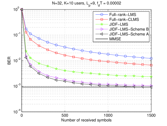
Figure 1: BER performance versus number of received symbols. Parameters of LMS algorithms: $\mu=0.05$ (full-rank), $\mu_{1}=0.01$, $\mu_{2}=0.25$ and $\mu_{a}=0.25$ (combination of full-rank), $B=8$, $I=3$, $D=4$, $\eta=0.005$ and $\mu=0.01$ (JIDF), $B=8$, $D_{1}=3$, $I_{1}=3$, $\eta_{1}=0.01$ and $\mu_{1}=0.1$, $D_{2}=6$, $I_{2}=6$, $\eta_{2}=0.01$ and $\mu_{2}=0.1$, $D_{3}=3$, $I_{3}=3$, $\eta_{3}=0.0075$, $\mu_{3}=0.01$, $D_{4}=6$, $I_{4}=6$, $\eta_{4}=0.0075$, $\mu_{4}=0.01$ (JIDF with Scheme A), $B=8$, $D_{1}=3$, $I_{1}=3$, $\eta_{1}=0.01$ and $\mu_{1}=0.1$, $D_{2}=6$, $I_{2}=6$, $\eta_{2}=0.0075$ and $\mu_{2}=0.01$ (JIDF with Scheme B).

In the second experiment, we assess the BER performance against the signal-to-noise-ratio (SNR) defined as $E_{b}/N_{0}$. Packets of $1500$ QPSK symbols are again transmitted and the curves are averaged over $100$ runs. The results depicted in Fig. 2 show that the proposed schemes A and B with the JIDF scheme can obtain significantly better performance than the JIDF without any combination for different values of SNR. From the results, we conclude that it might be more attractive to use Scheme B as it achieves a performance very close to Scheme A with half the complexity.

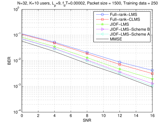
Figure 2: BER performance versus SNR. Parameters are optimized.

VI Conclusions

We proposed convex combination schemes for joint model-order and step-size adaptation of reduced-rank adaptive filters based on the JIDF method. The proposed schemes employ reduced-rank adaptive filters in parallel operating with different orders and step sizes, which are exploited by convex combination strategies. We investigated the performance of the proposed schemes in an interference suppression application for CDMA systems. Simulations showed that the proposed schemes significantly improve the performance of the existing reduced-rank adaptive filters based on the JIDF method.

References

• [1] S. Haykin,Adaptive Filter Theory, 4th ed.,Prentice- Hall, 2002.
• [2] J. Arenas-Garcia, A.R. Figueiras-Vidal, “Adaptive combination of normalised filters for robust system identification”, Electronics Letters vol. 41, no. 15, July 2005, pp. 874 - 875.
• [3] M.T.M. Silva, V.H. Nascimento, “Improving the tracking capability of adaptive filters via convex combination”, IEEE Trans. on Sig. Proc., vol. 56, no. 7, July 2008, pp. 3137 - 3149.
• [4] P. Strobach, “Low-rank adaptive filters”, IEEE Trans. on Sig. Proc., vol. 44, no. 12, Dec. 1996, pp. 2932 - 2947.
• [5] M. L. Honig and J. S. Goldstein, “Adaptive reduced-rank interference suppression based on the multistage Wiener filter,” IEEE Trans. on Communications, vol. 50, no. 6, June 2002.
• [6] D. A. Pados, G. N. Karystinos, “An iterative algorithm for the computation of the MVDR filter,” IEEE Trans. on Sig. Proc., vol. 49, No. 2, Feb. 2001.
• [7] R. C. de Lamare and R. Sampaio-Neto, “Adaptive reduced-rank MMSE filtering with interpolated FIR filters and adaptive interpolators”, IEEE Sig. Proc. Letters, vol. 12, no. 3, 2005, pp. 177 - 180.
• [8] R. C. de Lamare and R. Sampaio-Neto, “Adaptive Interference Suppression for DS-CDMA Systems based on Interpolated FIR Filters with Adaptive Interpolators in Multipath Channels”, IEEE Trans. Vehicular Technology, Vol. 56, no. 6, pp. 2457 - 2474, September 2007.
• [9] R. C. de Lamare and R. Sampaio-Neto, “Reduced-rank adaptive filtering based on joint iterative optimization of adaptive filters,” IEEE Sig. Proc. Letters, vol. 14, no. 12, Dec. 2007, pp. 980 - 983.
• [10] R. C. de Lamare and R. Sampaio-Neto, “Adaptive reduced-rank processing based on joint and iterative interpolation, decimation, and filtering”, IEEE Trans. on Sig. Proc., vol. 57, No. 7, July 2009, pp. 2503 - 2514.
• [11] M. Yukawa, R. C de Lamare and R. Sampaio-Neto, “Efficient acoustic echo cancellation with reduced-rank adaptive filtering based on selective decimation and adaptive interpolation”, IEEE Transactions on Audio, Speech, and Language Processing, vol. 16, no. 4, 2008, pp. 696-710.
• [12] T. S. Rappaport, Wireless Communications, Prentice-Hall, Englewood Cliffs, NJ, 1996.