ZU-TH 09/13

Soft-gluon resummation for single-particle inclusive
hadroproduction at high transverse momentum

Stefano Catani^(a), Massimiliano Grazzini^(b) and Alessandro Torre^(b)

^(a) INFN, Sezione di Firenze and Dipartimento di Fisica e Astronomia,

Università di Firenze, I-50019 Sesto Fiorentino, Florence, Italy

^(b) Institut für Theoretische Physik, Universität Zürich, CH-8057 Zürich, Switzerland

Abstract

We consider the cross section for one-particle inclusive production at high transverse momentum in hadronic collisions. We present the all-order resummation formula that controls the logarithmically-enhanced perturbative QCD contributions to the partonic cross section in the threshold region, at fixed rapidity of the observed parton (hadron). The explicit resummation up to next-to-leading logarithmic accuracy is supplemented with the computation of the general structure of the near-threshold contributions to the next-to-leading order cross section. This next-to-leading order computation allows us to extract the one-loop hard-virtual amplitude that enters into the resummation formula. This is a necessary ingredient to explicitly extend the soft-gluon resummation beyond the next-to-leading logarithmic accuracy. These results equally apply to both spin-unpolarized and spin-polarized scattering processes.

May 2013

1 Introduction

A well known feature of QCD is that perturbative computations for hard-scattering processes are sensitive to soft-gluon effects. These effects manifest themselves when the considered observable is computed close to its corresponding boundary of the phase space. In these kinematical regions, real radiation is strongly inhibited and the cancellation of infrared singular terms between virtual and real emission contributions is unbalanced. This leads to large logarithmic terms that can invalidate the (quantitative) reliability of the order-by-order perturbative expansion in powers of the QCD coupling $\alpha_{\mathrm{S}}$. These large logarithmic terms have to be evaluated at sufficiently-high perturbative orders and, whenever it is possible, they should be resummed to all orders in QCD perturbation theory.

In the context of hadron–hadron collisions, a class of soft-gluon sensitive observables is represented by inclusive hard-scattering cross sections in kinematical configurations that are close to (partonic) threshold. Typical examples are the cross sections for the production of Drell-Yan lepton pairs and Higgs bosons. In these cases, where only two QCD partons enter the hard-scattering subprocess at the Born level, the soft-gluon resummation formalism was established long ago [1, 2, 3], and explicit resummed results have been obtained up to next-to-next-to-leading logarithmic (NNLL) accuracy [4, 5, 6], and including still higher-order logarithmic terms that have been explicitly computed [7, 8]. The case of cross sections that are produced by Born-level hard scattering of three and four (or more) coloured partons is very important from the phenomenological viewpoint, and it is much more complex on the theoretical side. Soft-gluon dynamics leads to non-trivial colour correlations and colour coherence effects that depend on the colour flow of the underlying partonic subprocess. The general soft-gluon resummation formalism for inclusive cross sections in these complex multiparton processes was developed in a series of papers [9, 10, 11, 12, 13, 14]. In recent years, techniques and methods of Soft Collinear Effective Theory (SCET) have also been developed and applied to resummation for inclusive cross sections near (partonic) threshold [15, 16, 17, 18, 19, 20, 21].

Some examples of relevant processes with three or four partons at the Born level are the direct production of prompt photons [12, 13, 22, 23, 21], vector boson [24, 25] and Higgs boson [26] production at high transverse momentum, production of heavy quarks [9, 10, 12, 27, 20, 28, 29, 30] and coloured supersymmetric particles (Ref. [31] and references therein) at hadron colliders, single top-quark production [32, 33], jet [34, 35, 36] and dihadron [37, 38] production, and single-hadron inclusive production in hadronic collisions [39]. Soft-gluon resummation for single-hadron inclusive production in collisions of spin-polarized hadrons has been considered in Ref. [40].

In this paper we consider the single-hadron inclusive cross section. At sufficiently-large values of the hadron transverse momentum, the cross section for this process factorizes into the convolution of the parton distribution functions of the colliding hadrons with the (short-distance) partonic cross section and with the fragmentation function of the triggered parton into the observed hadron. Since the single inclusive cross section can be easily measured by experiments in hadron collisions, the process offers a relevant test of the QCD factorization picture. Conversely, measurements of the corresponding cross section as function of the transverse momentum and at different collision energies permit to extract quantitative information about the parton fragmentation (especially, the gluon fragmentation) function into the observed hadron, thus complementing the information obtained from hadron production in $e^{+}e^{-}$ and lepton-hadron collisions.

The next-to-leading order (NLO) QCD calculation of the cross section for single-hadron inclusive production was completed long ago [41, 42, 43]. Soft-gluon resummation of the logarithmically-enhanced contributions to the partonic cross section was performed in Ref. [39]. The study of Ref. [39] considers resummation for the transverse-momentum dependence of the cross section integrated over the rapidity of the observed final-state hadron, and it explicitly resums the leading-logarithmic (LL) and next-to-leading logarithmic (NLL) terms. The results of the phenomenological studies (which combine NLL resummation with the complete NLO calculation) in Ref. [39] indicate that the quantitative effect of resummation is rather large, especially in the kinematical configurations that are encountered in experiments at the typical energies of fixed-target collisions.

The content of the present paper aims at a twofold theoretical improvement on resummation for single-hadron inclusive production: we study soft-gluon resummation for the transverse-momentum cross section at fixed rapidity of the observed hadron (parton), and we extend the logarithmic accuracy of resummation by explicitly computing a class of logarithmic terms beyond the NLL accuracy. We first consider the structure of the NLO QCD corrections close to the partonic threshold. In this kinematical region, the initial-state partons have just enough energy to produce the triggered final-state parton (that eventually fragments into the observed hadron) and a small-mass recoiling jet, which is formed by soft and collinear partons. We perform the NLO calculation by using soft and collinear approximations, and we present a general expression for the logarithmically-enhanced terms (including the constant term) that correctly reproduces the known NLO result. Our NLO expression is directly factorized in colour space, and it allows us to explicitly disentangle colour-correlation and colour-interference effects that contribute to soft-gluon resummation at NLL and NNLL accuracy. We then consider the logarithmically-enhanced terms beyond the NLO. We use the formalism of Ref. [14], and we present the soft-gluon resummation formula that controls the logarithmic contributions to the rapidity distribution of the transverse-momentum cross section. The resummation formula is valid to arbitrary logarithmic accuracy, and it is explicitly worked out up to the NLL level. Finally, using our general expression of the NLO cross section, we determine the one-loop hard-virtual amplitude that enters into the colour-space factorization structure of the resummation formula. The colour interference between this one-loop amplitude and the NLL terms explicitly determines an entire class of resummed contributions at NNLL accuracy. Our study equally applies to both unpolarized and polarized scattering processes.

The paper is organized as follows. In Sect. 2 we introduce our notation. In Sect. 3 we present the result of our general NLO calculation of the partonic cross section. The resummation of the logarithmically-enhanced terms and the all-order resummation formula are presented and discussed in Sect. 4. Our results are briefly summarized in Sect. 5.

2 Single-particle cross section and notation

We consider the inclusive hard-scattering reaction

$$h_{1}(P_{1})+h_{2}(P_{2})\rightarrow h_{3}(P_{3})+X\;,$$ (1)

where the collision of the two hadrons $h_{1}$ and $h_{2}$ with momenta $P_{1}$ and $P_{2}$, respectively, produces the hadron $h_{3}$ with momentum $P_{3}$ accompanied by an arbitrary and undetected final state $X$. According to the QCD factorization theorem the corresponding cross section is given by

$$E_{3}\frac{d\sigma_{h_{3}}}{d^{3}{\bf P}_{3}}(P_{1},P_{2},P_{3}) =\sum_{a_{1},a_{2},a_{3}}\int_{0}^{1}dx_{1}\int_{0}^{1}dx_{2}\int_{0}^{1}\frac{dx_{3}}{x_{3}^{2}}\;f_{a_{1}/h_{1}}(x_{1},\mu_{F})\,f_{a_{2}/h_{2}}(x_{2},\mu_{F})\,d_{a_{3}/h_{3}}(x_{3},\mu_{f})$$

$$\times\;p^{0}_{3}\frac{d{\hat{\sigma}}_{a_{1}a_{2}\rightarrow a_{3}}}{d^{3}{\bf p}_{3}}(x_{1}P_{1},x_{2}P_{2},P_{3}/x_{3};\mu_{F},\mu_{f})\;,$$ (2)

where the index $a_{i}\,(i=1,2,3)$ denotes the parton species ($a=q,{\bar{q}},g$), $f_{a/h}(x,\mu_{F})$ is the parton density of the colliding hadron evaluated at the factorization scale $\mu_{F}$, and $d_{a/H_{3}}(x,\mu_{f})$ is the fragmentation function of the parton $a$ into the hadron $H_{3}$ at the factorization scale $\mu_{f}$ (in general, the fragmentation scale $\mu_{f}$ can be different from the scale $\mu_{F}$ of the parton densities). We use parton densities and fragmentation functions as defined in the ${\overline{\rm MS}}$ factorization scheme. The last factor, $d{\hat{\sigma}}_{a_{1}a_{2}\rightarrow a_{3}}(p_{1},p_{2},p_{3})$, on the right-hand side of Eq. (2) is the inclusive cross section for the partonic subprocess

$$a_{1}(p_{1})+a_{2}(p_{2})\rightarrow a_{3}(p_{3})+X\,\,,$$ (3)

which, throughout the paper, is always treated with massless partons (kinematics).

In Eq. (2), the partonic (hadronic) Lorentz-invariant phase space $d^{3}{\bf p}_{3}/p^{0}_{3}$ ($d^{3}{\bf P}_{3}/E_{3}$) is explicitly denoted in terms of the energy $p^{0}_{3}\,(E_{3})$ and the three-momentum ${\bf p}_{3}\,({\bf P}_{3})$ of the ‘detected’ final-state parton $a_{3}$ (hadron $h_{3}$). Other kinematical variables can equivalently be used. For instance, considering the centre–of–mass frame of the two colliding partons in the partonic subprocess of Eq. (3), we have

$$d^{3}{\bf p}_{3}/p^{0}_{3}=d\eta\;d^{2}{\bf p}_{T}\;\;,\quad\quad\eta=\frac{1}{2}\ln\frac{p_{3}\cdot p_{2}}{p_{3}\cdot p_{1}}\;\;,$$ (4)

where ${\bf p}_{T}$ is the transverse-momentum of the parton $a_{3}$ and $\eta$ is its rapidity (the forward region $\eta>0$ corresponds to the direction of the parton $a_{1}$). The kinematics of the partonic subprocess can also be described by using the customary Mandelstam variables $s,t,u$:

$$s=(p_{1}+p_{2})^{2}~{},~{}~{}~{}t=(p_{1}-p_{3})^{2}~{},~{}~{}~{}u=(p_{2}-p_{3})^{2}~{},$$ (5)

with the phase-space boundaries

$$s\geq 0~{},~{}~{}~{}t\leq 0~{},~{}~{}~{}u\leq 0~{},~{}~{}~{}s+t+u\geq 0\;\;.$$ (6)

Analogous kinematical variables can be introduced for the corresponding hadronic process in Eq. (1). Throughout the paper, hadronic and partonic kinematical variables are typically denoted by the same symbol, although we use capital letters for hadronic variables. For instance, $S=(P_{1}+P_{2})^{2}$ is the square of the centre–of–mass energy of the hadronic collision and ${\bf P}_{3T}={\bf P}_{T}$ is the transverse momentum of the observed hadron $h_{3}$.

The partonic cross section $d{\hat{\sigma}}_{a_{1}a_{2}\rightarrow a_{3}}$ depends on the factorization scales, and it is computable in QCD perturbation theory as power series expansion in the QCD coupling $\alpha_{\mathrm{S}}(\mu_{R}^{2})$ ($\mu_{R}$ denotes the renormalization scale, and we use the ${\overline{\rm MS}}$ renormalization scheme). The perturbative expansion starts at ${\cal O}(\alpha_{\mathrm{S}}^{2})$ since the leading order (LO) partonic process corresponds to the $2\rightarrow 2$ reaction $a_{1}a_{2}\rightarrow a_{3}a_{4}$. Considering the expansion up to the next-to-leading order (NLO), we write

$$\!\!\!d{\hat{\sigma}}_{a_{1}a_{2}\rightarrow a_{3}}(p_{1},p_{2},p_{3};\mu_{F},\mu_{f})=\alpha_{\mathrm{S}}^{2}(\mu_{R}^{2})\!\!\!\!\!\! \!\!\!\Bigl{(}\;d{\hat{\sigma}}_{a_{1}a_{2}\rightarrow a_{3}a_{4}}^{(0)}(p_{1},p_{2},p_{3})\Bigr{.}$$

$$\!\!+\Bigl{.}\;\frac{\alpha_{\mathrm{S}}(\mu_{R}^{2})}{2\pi}\,d{\hat{\sigma}}^{(1)}_{a_{1}a_{2}\rightarrow a_{3}}(p_{1},p_{2},p_{3};\mu_{R},\mu_{F},\mu_{f})+{\cal O}(\alpha_{\mathrm{S}}^{2})\Bigr{)}\,.$$

The LO term $d{\hat{\sigma}}_{a_{1}a_{2}\rightarrow a_{3}a_{4}}^{(0)}$ is directly related (see Eq. (19)) to the Born-level scattering amplitude of the partonic reaction $a_{1}a_{2}\rightarrow a_{3}a_{4}$. The NLO term $d{\hat{\sigma}}^{(1)}_{a_{1}a_{2}\rightarrow a_{3}}$ is known: the contribution of the partonic subprocess with non-identical quarks was computed in Refs. [41, 42], and the complete NLO calculation for all partonic subprocesses was presented in Ref. [43].

The NLO calculation was carried out in analytical form, and it is presented [41, 42, 43] in terms of the independent kinematical variables $s,v$ and $w$, which are related to the Mandelstam variables of Eq. (5) through the definition

$$v\equiv 1+t/s~{},~{}~{}~{}~{}~{}~{}~{}~{}w\equiv-u/(s+t)\,\,,$$ (8)

with the corresponding phase-space boundaries

$$s\geq 0~{},~{}~{}~{}1\geq v\geq 0~{},~{}~{}~{}1\geq w\geq 0\;\;.$$ (9)

Using these variables, the partonic cross section in Eqs. (2) and (2) can be written as

$$p^{0}_{3}\frac{d{\hat{\sigma}}}{d^{3}{\bf p}_{3}}(p_{1},p_{2},p_{3};\mu_{F},\mu_{f})=\frac{\alpha_{\mathrm{S}}^{2}(\mu_{R}^{2})}{\pi\,s} \!\!\!\!\!\!\Bigl{[}\;\frac{1}{v}\frac{d{\hat{\sigma}}^{(0)}(s,v)}{dv}\;\delta(1-w)\Bigr{.}$$

$$\!\!\!\!\!\!+\Bigl{.}\;\frac{\alpha_{\mathrm{S}}(\mu_{R}^{2})}{2\pi}\;\frac{1}{v\,s}\;{\cal C}^{(1)}(s,v,w;\mu_{R},\mu_{F},\mu_{f})+{\cal O}(\alpha_{\mathrm{S}}^{2})\Bigr{]}\,\,,$$

where the flavour indices are left understood (the term in the square bracket exactly corresponds to the square-bracket term in Eq. (10) of Ref. [43], modulo the overall factor $\alpha_{\mathrm{S}}^{2}(\mu_{R}^{2})$). The first term in the square bracket of Eq. (2) is the Born-level contribution, and the function ${\cal C}^{(1)}$ encodes the NLO corrections.

The Born-level term in Eq. (2) has a sharp integrable singularity at $w=1$. This singularity has a kinematical origin. Indeed $(1-w)$ is proportional (see Eq. (8)) to $s_{X}=s+t+u$, which is the invariant mass squared of the QCD radiation (i.e. the unobserved final-state system $X$ in Eq. (3)) recoiling against the ‘observed’ final-state parton $a_{3}$. At the LO, the system $X$ is formed by a single massless parton $a_{4}(p_{4})$ and, therefore, $s_{X}=p_{4}^{2}$ exactly vanishes thus leading to the factor $\delta(1-w)$ in Eq. (2). At higher perturbative orders, the LO singularity at $w\rightarrow 1$ is enhanced by logarithmic terms of the type $\ln(1-w)$. The enhancement has a dynamical origin, and it is produced by soft-gluon radiation. Indeed, in the kinematical region where $w\rightarrow 1$, the system $X$ is forced to carry a very small invariant mass, and the associated production of hard QCD radiation is strongly suppressed. The associated production of soft QCD radiation is instead allowed and, due to the soft-gluon bremsstrahlung spectrum, it generates large logarithmic corrections.

The presence of logarithmically-enhanced terms is evident from the known NLO result. The structure of the NLO term ${\cal C}^{(1)}$ in Eq. (2) is customarily written (see, e.g., Eqs. (10) and (22) in Ref. [43]) in the following form:

$${\cal C}^{(1)}(s,v,w;\mu_{R},\mu_{F},\mu_{f}) = {\cal C}_{3}(v)\left(\frac{\ln(1-w)}{1-w}\right)_{+}+{\cal C}_{2}(v;s,\mu_{F},\mu_{f})\left(\frac{1}{1-w}\right)_{+}$$ (11)

$$+ {\cal C}_{1}(v;s,\mu_{R},\mu_{F},\mu_{f})\,\delta(1-w)+{\cal C}_{0}(1-w,v;s,\mu_{R},\mu_{F},\mu_{f})\,.$$

The last term on the right-hand side is a non-singular function of $w$ in the limit $w\rightarrow 1$, namely, ${\cal C}_{0}(1-w,v)={\cal O}\left((1-w)^{0}\right)$ (see Refs. [41, 42] for explicit expressions in analytic form). The functions ${\cal C}_{3}$, ${\cal C}_{2}$ and ${\cal C}_{1}$ do not depend on $w$, and they multiply functions of $w$ that are singular (and logarithmically-enhanced) at $w\rightarrow 1$. These singular functions are expressed by $\delta(1-w)$ and customary ‘plus-distributions’, $[(\ln^{k}(1-w))/(1-w)]_{+}\,$, defined over the range $1\geq w\geq 0$.

In this paper we deal with the perturbative QCD contributions beyond the NLO, in the kinematical region where $w\rightarrow 1$ or, more generally, $s_{X}\rightarrow 0$. This region is usually referred to as the region of partonic threshold, since the partonic process in Eq. (3) approaches the near-elastic limit. The observed parton $a_{3}$ is produced with the maximal energy that is kinematically allowed by momentum conservation, and the recoiling partonic system $X$ has the minimal invariant mass. We are interested in the near-threshold behaviour of the partonic cross section, and we compute the higher-order contributions that dominate near the partonic threshold. Before considering the higher-order terms, in Sect. 3 we focus on the behaviour of the NLO cross section, and we present the results of our independent NLO calculation in the kinematical region close to the partonic threshold. Our NLO results are obtained and expressed in a form that is suitable (and necessary) for the all-order treatment and resummation of the logarithmically-enhanced QCD corrections.

The discussion in this section has been limited to the case in which the inclusive hard-scattering reaction in Eq. (1) is unpolarized. The same discussion applies to polarized process in which one or more of the three hadrons $h_{1},h_{2}$ and $h_{3}$ have definite states of spin polarizations. The only difference between the unpolarized and polarized cases is that the parton densities, the fragmentation function and the partonic cross section in the factorization formula (2) have to be replaced by the corresponding spin-polarized quantities. The structure of the threshold behaviour of the polarized partonic cross section is completely analogous to that of Eqs. (2) and (11) (see, e.g., Ref. [40] and references therein) In the following sections, we continue our discussion by explicitly considering the unpolarized case. Our results equally apply to both unpolarized and polarized cross sections. At the end of Sect. 4 (just before Sect. 4.1), we briefly comment on soft-gluon resummation for the polarized case, and we summarize the technical differences between unpolarized and polarized scattering processes.

3 NLO results near partonic threshold

In the near-threshold region, the NLO partonic cross section of Eq. (2) is controlled by the functions ${\cal C}_{3},{\cal C}_{2}$ and ${\cal C}_{1}$ in Eq. (11) and, more precisely, each of these functions depends on the various flavour channels that contribute to the partonic reaction $a_{1}a_{2}\rightarrow a_{3}a_{4}$. The functions ${\cal C}_{i,a_{1}a_{2}\rightarrow a_{3}a_{4}}(v)$ with $i=1,2,3$ are all reported in Sect. 3 of Ref. [43]. The corresponding analytic expressions have a rather involved dependence (especially for ${\cal C}_{1}$) on $v$, colour factors and the flavour channel.

We have performed an independent calculation of the NLO cross section near threshold. We have computed the three coefficients of the logarithmic expansion in Eq. (11), including the coefficient ${\cal C}_{1}$ that controls the term proportional to $\delta(1-w)$. The final result is presented in this section, and it has a rather compact form. More importantly, it embodies an amount of process-independent information that cannot be extracted (or, say, it is difficult to be extracted) from the results of Ref. [43]. In particular, our calculation and the ensuing result keep explicitly under control colour correlation effects that are a typical and general feature of soft-gluon radiation from $2\rightarrow 2$ parton scattering processes. The knowledge of these colour correlation terms is essential (see Sect. 4) to compute logarithmically-enhanced contributions beyond the NLO.

At the NLO, the parton cross section receives contributions from two types of partonic processes. The elastic process

$$a_{1}(p_{1})+a_{2}(p_{2})\rightarrow a_{3}(p_{3})+a_{4}(p_{4})\,\,,$$ (12)

which has to be evaluated with one-loop virtual corrections, and the inelastic process in Eq. (3) with real emission of $X=\{2~{}{\rm partons}\}$, which is evaluated at the tree level. Virtual and real contributions are separately divergent, and we use dimensional regularization with $d=4-2\epsilon$ space-time dimensions to deal with both ultraviolet and infrared (IR) divergences. The elastic process contributes only to the term proportional to $\delta(1-w)$ in Eq. (11), and its contribution is directly proportional to the (ultraviolet) renormalized one-loop scattering amplitude of the four-parton process. In the threshold region $w\rightarrow 1$, the five-parton inelastic process gives dominant contributions only from two kinematical configurations of the system $X=\{2~{}{\rm partons}\}$: either one of the two partons is soft or both partons are collinear. We treat these two configurations by using soft and collinear factorization formulae (in colour space) [44] of the scattering amplitudes, and we perform the phase-space integration. This real emission term is finally combined with the collinear-divergent counterterms necessary to define the NLO parton densities and fragmentation function and with the virtual correction from the four-parton elastic process. The final result, which is IR finite, has a factorized structure: it is given in terms of flavour and colour-space factors that acts on the scattering amplitude of the four-parton elastic process.

To present the result of our NLO calculation in its factorized form, we need to briefly recall the representation of the four-parton scattering amplitude in the colour-space notation [44, 45]. The all-loop QCD amplitude ${\cal M}$ of the scattering process in Eq. (12) is written as

$$|{\cal M}_{a_{1}a_{2}a_{3}a_{4}}\rangle=\alpha_{\mathrm{S}}(\mu_{R}^{2})\left[|{\cal M}^{(0)}_{a_{1}a_{2}a_{3}a_{4}}\rangle+\sum_{n=1}^{\infty}\left(\frac{\alpha_{\mathrm{S}}(\mu_{R}^{2})}{2\pi}\right)^{n}|{\cal M}^{(n)}_{a_{1}a_{2}a_{3}a_{4}}(\mu_{R})\rangle\right]\;\;,$$ (13)

where ${\cal M}^{(0)}$ is the Born-level contribution, ${\cal M}^{(n)}$ is the contribution at the $n$-loop level, and we always consider the renormalized (in the ${\overline{\rm MS}}$ scheme) amplitude. The remaining IR divergences are regularized in $d=4-2\epsilon$ space-time dimensions by using the customary scheme of conventional dimensional regularization (CDR) [46]. The subscript ‘$a_{1}a_{2}a_{3}a_{4}$’ refers to the flavour of the four partons, while the dependence on the parton momenta $p_{i}$ $(i=1,\dots,4)$ is not explicitly denoted. Note, however, that the elastic $2\rightarrow 2$ process is evaluated exactly at the partonic threshold (i.e. with $s+t+u=0$), and momentum conservation ($p_{1}+p_{2}=p_{3}+p_{4}$) implies that ${\cal M}$ only depends on two kinematical variables (e.g., it depends on $s$ and $v$).

The colour indices $c_{i}$ of the partons are embodied [44, 45] in the ‘ket’ notation, through the definition

$${\cal M}_{a_{1}a_{2}a_{3}a_{4}}^{c_{1}c_{2}c_{3}c_{4}}\equiv\langle\,c_{1}c_{2}c_{3}c_{4}|{\cal M}_{a_{1}a_{2}a_{3}a_{4}}\rangle\;\;,$$ (14)

so that $|\cdots\rangle$ is an abstract vector in colour space, and $\langle\cdots|$ is its complex-conjugate vector. Gluon radiation from the parton with momentum $p_{i}$ is described by the colour-charge matrix $({\mbox{\boldmath$T$}}_{i})^{c}$ ($c$ is the colour index of the radiated gluon) and colour conservation implies

$$\sum_{i=1}^{4}\;{\mbox{\boldmath$T$}}_{i}\;|{\cal M}_{a_{1}a_{2}a_{3}a_{4}}\rangle=0\;\;.$$ (15)

Note that according to this notation the colour flow is treated as ‘outgoing’, so that ${\mbox{\boldmath$T$}}_{3}$ and ${\mbox{\boldmath$T$}}_{4}$ are the colour charges of the partons $a_{3}$ and $a_{4}$, while ${\mbox{\boldmath$T$}}_{1}$ and ${\mbox{\boldmath$T$}}_{2}$ are the colour charges of the anti-partons ${\overline{a}}_{1}$ and ${\overline{a}}_{2}$. The colour-charge algebra for the product $({\mbox{\boldmath$T$}}_{i})^{c}({\mbox{\boldmath$T$}}_{j})^{c}\equiv{\mbox{\boldmath$T$}}_{i}\cdot{\mbox{\boldmath$T$}}_{j}$ gives

$${\mbox{\boldmath$T$}}_{i}^{2}=C_{a_{i}}\;,\quad\quad\quad\quad C_{g}=C_{A}\;,\;\;\;C_{q}=C_{\bar{q}}=C_{F}\;,$$ (16)

where $C_{a}$ is the Casimir factor and, in $SU(N_{c})$ QCD, we have $C_{a}=N_{c}$ if $a$ is a gluon and $C_{a}=C_{F}=(N_{c}^{2}-1)/(2N_{c})$ if $a$ is a quark or an antiquark. Thus, ${\mbox{\boldmath$T$}}_{i}^{2}$ is a $c$-number term or, more precisely, a multiple of the unit matrix in colour space. Non-trivial colour correlations are produced by the quadratic operators ${\mbox{\boldmath$T$}}_{i}\cdot{\mbox{\boldmath$T$}}_{j}={\mbox{\boldmath$T$}}_{j}\cdot{\mbox{\boldmath$T$}}_{i}$ with $i\neq j$. These are six different operators, but, due to colour conservation (i.e. Eq. (15)), only two of them lead to colour correlations that are linearly independent (see the Appendix A of Ref. [44]). Two linearly independent operators are ${\mbox{\boldmath$T$}}_{1}\cdot{\mbox{\boldmath$T$}}_{3}$ and ${\mbox{\boldmath$T$}}_{2}\cdot{\mbox{\boldmath$T$}}_{3}$. Different choices of pairs (e.g., the pair ${\mbox{\boldmath$T$}}_{1}\cdot{\mbox{\boldmath$T$}}_{2}$ and ${\mbox{\boldmath$T$}}_{1}\cdot{\mbox{\boldmath$T$}}_{3}$) of independent operators are feasible and physically equivalent. For instance, by analogy with the Mandelstam kinematical variables of the $2\rightarrow 2$ parton scattering, we can use [47] the $s$- , $t$-  and $u$-channel colour-correlation operators ${\bf T}_{s}^{2}$, ${\bf T}_{t}^{2}$ and ${\bf T}_{u}^{2}$,

$${\bf T}_{s}^{2} = \left({\bf T}_{1}+{\bf T}_{2}\right)^{2}=\left({\bf T}_{3}+{\bf T}_{4}\right)^{2}\;\;,$$

$${\bf T}_{t}^{2} = \left({\bf T}_{1}+{\bf T}_{3}\right)^{2}=\left({\bf T}_{2}+{\bf T}_{4}\right)^{2}\;\;,$$ (17)

$${\bf T}_{u}^{2} = \left({\bf T}_{2}+{\bf T}_{3}\right)^{2}=\left({\bf T}_{1}+{\bf T}_{4}\right)^{2}\;\;,$$

which are linearly related by colour conservation:

$${\bf T}_{s}^{2}+{\bf T}_{t}^{2}+{\bf T}_{u}^{2}=\sum_{i=4}^{4}{\bf T}_{i}^{2}=\sum_{i=4}^{4}C_{a_{i}}\;\;.$$ (18)

The LO cross section in Eq. (2) depends on the square of the Born-level scattering amplitude $|{\cal M}^{(0)}\rangle$:

$$\frac{d{\hat{\sigma}}^{(0)}_{a_{1}a_{2}\rightarrow a_{3}a_{4}}(s,v)}{dv}=\frac{1}{N^{(in)}_{a_{1}a_{2}}}\;\frac{1}{16\pi\,s}\;|{\cal M}^{(0)}_{a_{1}a_{2}a_{3}a_{4}}|^{2}\;\;,$$ (19)

where $|{\cal M}^{(0)}|^{2}=\langle{\cal M}^{(0)}\;|\;{\cal M}^{(0)}\rangle$ and the factor $N^{(in)}_{a_{1}a_{2}}=4\,n_{c}(a_{1})\,n_{c}(a_{2})$ comes from the average over the spins and colours ($n_{c}(q)=n_{c}({\bar{q}})=N_{c},n_{c}(g)=N_{c}^{2}-1$) of the initial-state partons $a_{1}$ and $a_{2}$.

The Born-level and one-loop ($|{\cal M}^{(1)}\rangle$) scattering amplitudes of the partonic reaction $a_{1}a_{2}\rightarrow a_{3}a_{4}$ are known [48, 49]. The one-loop scattering amplitude includes IR-divergent terms that have a process-independent (universal) structure [50, 45]. The NLO contribution ${\cal C}^{(1)}$ in Eq. (2) depends on the IR-finite part ${\cal M}^{(1)\,{\rm fin}}$ of the one-loop scattering amplitude. The IR-finite part is obtained through the factorization formula [45]

$$|{\cal M}^{(1)}\rangle={{\mbox{\boldmath$I$}}}_{\rm sing}^{(1)}\;|{\cal M}^{(0)}\rangle+|{\cal M}^{(1)\,{\rm fin}}\rangle\;,$$ (20)

where the colour operator ${{\mbox{\boldmath$I$}}}^{(1)}_{\rm sing}$ embodies the one-loop IR divergence in the form of double and single poles ($1/\epsilon^{2}$ and $1/\epsilon$), while ${\cal M}^{(1)\,{\rm fin}}$ is finite as $\epsilon\rightarrow 0$. To specify the expression of ${\cal M}^{(1)\,{\rm fin}}$ in an unambiguous way, the contributions of ${\cal O}(\epsilon^{0})$ that are included in ${{\mbox{\boldmath$I$}}}^{(1)}_{\rm sing}$ must be explicitly defined. We use the expression

$${{\mbox{\boldmath$I$}}}^{(1)}_{\rm sing}=\frac{1}{2}\frac{1}{\Gamma(1-\epsilon)}\left[\frac{1}{\epsilon^{2}}\sum_{\begin{subarray}{c}i,j=1\\ i\,\neq\,j\end{subarray}}^{4}{\mbox{\boldmath$T$}}_{i}\cdot{\mbox{\boldmath$T$}}_{j}\left(\frac{4\pi\mu_{R}^{2}\,e^{-i\lambda_{ij}\pi}}{2p_{i}\cdot p_{j}}\right)^{\epsilon}-\frac{1}{\epsilon}\sum_{i=1}^{4}\gamma_{a_{i}}\left(\frac{4\pi\mu_{R}^{2}\,s}{u\,t}\right)^{\epsilon}\right]\;\;,$$ (21)

where $e^{-i\lambda_{ij}\pi}$ is the unitarity phase factor ($\lambda_{ij}=-1$ if $i$ and $j$ are both incoming or outgoing partons and $\lambda_{ij}=0$ otherwise), and the flavour dependent coefficients $\gamma_{a}$ are ($n_{F}$ is the number of flavours of massless quarks)

$$\gamma_{q}=\gamma_{\bar{q}}=\frac{3}{2}C_{F}~{}~{},~{}~{}~{}~{}~{}~{}\gamma_{g}=\frac{11}{6}C_{A}-\frac{1}{3}n_{F}\;\;.$$ (22)

Note that the operator ${{\mbox{\boldmath$I$}}}^{(1)}_{\rm sing}$ in Eq. (21) differs from the operator ${{\mbox{\boldmath$I$}}}^{(1)}$ used in Ref. [45]: the difference is IR finite, and it is due to terms of ${\cal O}(\epsilon^{0})$ that are proportional to the coefficients $\gamma_{a_{i}}$. The effect of this difference is absorbed in $|{\cal M}^{(1)\,{\rm fin}}\rangle$.

The term ${\cal C}^{(1)}$ in Eq. (2) is IR finite, and the final result of our NLO calculation is expressed by the following colour-space factorization formula:

$$16\pi\,N^{(in)}\;{\cal C}^{(1)}=\langle{\cal M}^{(0)}|\,{{\mbox{\boldmath$C$}}}^{(1)}|{\cal M}^{(0)}\rangle+\left(\langle{\cal M}^{(0)}|{\cal M}^{(1)\,{\rm fin}}\rangle+{\rm c.c.}\right)\delta(1-w)+{\cal O}\left((1-w)^{0}\right)\,,$$ (23)

where ${\rm c.c.}$ stands for complex conjugate, and the flavour indices are left understood. The function ${{\mbox{\boldmath$C$}}}^{(1)}$ (reinserting the dependence on flavour indices and kinematical variables, we actually have ${{\mbox{\boldmath$C$}}}^{(1)}\rightarrow{{\mbox{\boldmath$C$}}}^{(1)}_{a_{1}a_{2}a_{3}a_{4}}(s,v,w;\mu_{R},\mu_{F},\mu_{f})$) has the form of a colour-space operator. We find the result:

$${{\mbox{\boldmath$C$}}}^{(1)}_{a_{1}a_{2}a_{3}a_{4}}(s,v,w;\mu_{R},\mu_{F},\mu_{f}) =2{\left(\frac{\ln(1-w)}{1-w}\right)_{+}}\bigg{[}\,2\sum_{i=1}^{3}{\mbox{\boldmath$T$}}_{i}^{2}-{\mbox{\boldmath$T$}}_{4}^{2}\,\bigg{]}$$

$$-{\left(\frac{1}{1-w}\right)_{+}}\bigg{[}\,2\sum_{i=1}^{3}{\mbox{\boldmath$T$}}_{i}^{2}\left(\ln\frac{1-v}{v}+\ln\frac{\mu_{Fi}^{2}}{s}\right)-2\,{\mbox{\boldmath$T$}}_{4}^{2}\ln(1-v)$$

$$+\gamma_{a_{4}}+8\,\Big{(}{\mbox{\boldmath$T$}}_{1}\cdot{\mbox{\boldmath$T$}}_{3}\ln(1-v)+{\mbox{\boldmath$T$}}_{2}\cdot{\mbox{\boldmath$T$}}_{3}\,\ln v\Big{)}\,\bigg{]}$$

$$+\delta(1-w)\Bigg{\{}\frac{\pi^{2}}{2}\left({\mbox{\boldmath$T$}}_{1}^{2}+{\mbox{\boldmath$T$}}_{2}^{2}+3{\mbox{\boldmath$T$}}_{3}^{2}-\frac{4}{3}{\mbox{\boldmath$T$}}_{4}^{2}\right)$$

$$-2{\mbox{\boldmath$T$}}_{3}^{2}\ln v\,\ln\frac{\mu_{f}^{2}}{s}+2{\mbox{\boldmath$T$}}_{2}^{2}\ln\frac{1-v}{v}\ln\frac{\mu_{F}^{2}}{s}-\sum_{i=1}^{3}\gamma_{a_{i}}\ln\frac{\mu_{Fi}^{2}}{s\,v(1-v)}$$

$$+\ln v\ln(1-v)\left({\mbox{\boldmath$T$}}_{4}^{2}-{\mbox{\boldmath$T$}}_{1}^{2}-{\mbox{\boldmath$T$}}_{2}^{2}-{\mbox{\boldmath$T$}}_{3}^{2}\right)$$

$$+\ln^{2}(1-v)\left({\mbox{\boldmath$T$}}_{1}^{2}+{\mbox{\boldmath$T$}}_{3}^{2}-{\mbox{\boldmath$T$}}_{4}^{2}\right)+\ln^{2}v\,({\mbox{\boldmath$T$}}_{2}^{2}+{\mbox{\boldmath$T$}}_{3}^{2})+\gamma_{a_{4}}\ln(1-v)$$

$$+{\mbox{\boldmath$T$}}_{1}\cdot{\mbox{\boldmath$T$}}_{3}\Bigl{(}2\pi^{2}+2\ln(1-v)\left(\ln(1-v)-2\ln v\right)\Bigr{)}$$

$$+{\mbox{\boldmath$T$}}_{2}\cdot{\mbox{\boldmath$T$}}_{3}\Bigl{(}2\pi^{2}+2\ln v\left(2\ln(1-v)-3\ln v\right)\Bigr{)}+K_{a_{4}}\Bigg{\}}\,,$$ (24)

where we have defined

$$\mu_{F1}=\mu_{F2}=\mu_{F}~{}~{},~{}~{}~{}~{}~{}~{}~{}\mu_{F3}=\mu_{f}\;,$$ (25)

and the flavour dependent coefficients $K_{a}$ are given by

$$K_{q}=K_{\bar{q}}=\left(\frac{7}{2}-\frac{\pi^{2}}{6}\right)C_{F}~{}~{},~{}~{}~{}~{}~{}K_{g}=\left(\frac{67}{18}-\frac{\pi^{2}}{6}\right)C_{A}-\frac{5}{9}\,n_{F}\;.$$ (26)

The result in Eq. (3) contains terms that are proportional to plus-distributions of $w$ (the action of these terms onto the Born-level scattering amplitude as in Eq. (23) directly gives the coefficients ${\cal C}_{3}$ and ${\cal C}_{2}$ in Eq. (11)) and a term that is proportional to $\delta(1-w)$. The sum of the latter term and the analogous term (which is proportional to ${\cal M}^{(1)\,{\rm fin}}$) on the right-hand side of Eq. (23) gives the function ${\cal C}_{1}$ in Eq. (11) (note that a change in the definition of ${\cal M}^{(1)\,{\rm fin}}$ would be compensated by a corresponding change in ${{\mbox{\boldmath$C$}}}^{(1)}$, so that the total NLO result in Eqs. (11) and (23) is unchanged).

All the contributions to the NLO colour-space function ${{\mbox{\boldmath$C$}}}^{(1)}$ in Eq. (3) have a definite physical origin. The terms that are proportional to the colour charges ${\mbox{\boldmath$T$}}_{i}$ are due to radiation (either collinear or at wide angles) of soft gluons. In particular, the coefficients of $(1/(1-w))_{+}$ and $\delta(1-w)$ depend on colour correlation operators. In Eq. (3), we have used the two linearly independent operators ${\mbox{\boldmath$T$}}_{1}\cdot{\mbox{\boldmath$T$}}_{3}$ and ${\mbox{\boldmath$T$}}_{2}\cdot{\mbox{\boldmath$T$}}_{3}$ to explicitly present the colour correlation contributions. The terms that are proportional to the flavour-dependent coefficients $\gamma_{a}$ and $K_{a}$ have a collinear (and non-soft) origin. In particular, we recall (see Eq. (C.13) in Appendix C of Ref. [44]) that $K_{a}$ is related to the $(d-4)$-dimensional part (i.e. the terms of ${\cal O}(\epsilon)$) of the LO collinear splitting functions. We also remark and recall (see Eq. (7.28) and related comments in Ref. [44]) that the gluonic coefficient $K_{g}$ in Eq. (26) is exactly equal to the coefficient $K$ (see Eqs. (40) and (63)) that controls the intensity of soft-gluon radiation at ${\cal O}(\alpha_{\mathrm{S}}^{2})$.

In the case of the four-parton scattering $a_{1}a_{2}\rightarrow a_{3}a_{4}$, our process-independent NLO results can be checked by comparison with the NLO results of Ref. [43]. Using Eqs. (20), (23) and (3) and the one-loop virtual contributions from Ref. [46], we have verified that we correctly reproduce the results of Ref. [43] for the NLO coefficient ${\cal C}^{(1)}$ of the various partonic channels (note that the expressions of Ref. [43] have to be converted to the ${\overline{\rm MS}}$ factorization scheme, since they explicitly refer to a different factorization scheme).

An additional check can be carried out by considering the case in which the parton $a_{3}$ is replaced by a photon. In this case ${\mbox{\boldmath$T$}}_{3}=0$, and the colour algebra becomes trivial (the colour correlation terms ${\mbox{\boldmath$T$}}_{1}\cdot{\mbox{\boldmath$T$}}_{3}$ and ${\mbox{\boldmath$T$}}_{2}\cdot{\mbox{\boldmath$T$}}_{3}$ vanish). Using the one-loop virtual contribution for the process $gq\rightarrow\gamma q$ [51] and its crossing-related channels, we have explicitly verified that the results in Eqs. (20), (23) and (3) correctly reproduces the NLO coefficient of the cross section for prompt-photon production [52, 53].

4 All-order soft-gluon resummation

In the near-threshold region $w\rightarrow 1$, the singular behaviour of the NLO partonic cross section is further enhanced at higher perturbative orders. Radiation of soft and collinear partons can produce (at most) two additional powers of $\ln(1-w)$ for each additional power of $\alpha_{\mathrm{S}}$. A reliable evaluation of the partonic cross section in the near-threshold region requires the computation and, possibly, the all-order resummation of these large logarithmic contributions.

Note that we are considering the partonic (and not the hadronic) cross section in its near-threshold region. The available partonic phase space is smaller than the hadronic phase space. Therefore, if the hadronic process in Eq. (1) is studied in kinematical configurations close to its threshold (roughly speaking, the region where $P_{3T}\simeq{\sqrt{S}}/2$), the partonic process in Eq. (3) is also kinematically forced toward its threshold. In these kinematical configurations, the behaviour of the hadronic cross section is certainly dominated by the large logarithmic contributions. Nonetheless, as is well known, these partonic logarithmic contributions typically (see, e.g., Ref. [39]) give the bulk of the radiative corrections to the hadronic process also in kinematical configurations that are not close to the hadronic threshold. This effect is due to the convolution structure with the parton densities and the fragmentation function according to Eq. (2). Roughly speaking, the partonic threshold corresponds to the region where $p_{3T}\simeq{\sqrt{s}}/2$, which can be rewritten in terms of hadronic variables ($p_{3T}=P_{3T}/x_{3}\;,s=x_{1}x_{2}S$ as in Eq. (2)) and it translates into the region where $P_{3T}\simeq x_{3}{\sqrt{x_{1}x_{2}}}{\sqrt{S}}/2$ . Since the typical average values of momentum fractions $x_{i}$ ($i=1,2,3$) that mostly contribute to Eq. (2) are small (parton densities and fragmentation functions are indeed strongly suppressed at large values of $x$), the partonic threshold region $P_{3T}\simeq x_{3}{\sqrt{x_{1}x_{2}}}{\sqrt{S}}/2$ can give the dominant contribution to the hadronic cross section even if $P_{3T}\ll{\sqrt{S}}/2$, namely, in kinematical configurations that are far from the hadronic threshold.

The three independent kinematical variables $\{\,s,v,w\,\}$ (which are customarily used to present the NLO results) are not particularly suitable for an all-order treatment near threshold, because of their degree of asymmetry under the exchange $u\leftrightarrow t$. The all-order treatment of the terms $\ln^{n}(1-w)$ unavoidably produces an asymmetry with respect to $u\leftrightarrow t$ (see Eq. (8)). In practical applications of resummation, this feature can lead to (quantitatively) non-negligible and unphysical asymmetries in the angular (rapidity) distribution of the produced hadron $h_{3}$. We note that this asymmetry effect is formally suppressed by powers of $(1-w)$ only after the complete resummation of the entire perturbative series of logarithmic terms to all orders in $\alpha_{\mathrm{S}}$. Any feasible resummed calculations involve the truncation of the all-order series to some level of logarithmic accuracy and, in this case, the asymmetry effect is suppressed only by subleading (but still singular) logarithmic contributions (see Eqs. (30) and (31)).

We introduce the three independent kinematical variables $\{\,x_{\omega},r,p_{T}^{2}\,\}$ that are defined by

$$x_{\omega}=-\frac{u+t}{s}~{},~{}~{}~{}~{}r=\frac{u}{t}~{},~{}~{}~{}~{}p_{T}^{2}=\frac{ut}{s}\;,$$ (27)

with the corresponding phase-space boundaries

$$1\geq x_{\omega}\geq 0~{},~{}~{}~{}~{}r\geq 0~{},~{}~{}~{}~{}p_{T}^{2}\geq 0\;.$$ (28)

The variable $p_{T}$ is the transverse momentum of the observed parton $a_{3}$ (see Eq. (4)). In the centre–of–mass frame of the partonic collision in Eq. (3), the variable $x_{\omega}=2\,p_{3}^{0}/{\sqrt{s}}$ is the energy fraction of the parton $a_{3}$ and $r=(1+\cos\theta^{*}_{13})/(1-\cos\theta^{*}_{13})$ is related to its scattering angle $\theta^{*}_{13}$. The relation with the transverse momentum and rapidity of the parton $a_{3}$ (see Eq. (4)) is

$$x_{\omega}=\frac{2\,p_{T}}{{\sqrt{s}}}\cosh\eta~{},~{}~{}~{}~{}r=e^{2\eta}\;.$$ (29)

In terms of the kinematical variables in Eq. (27), the near-threshold limit $s_{X}=s+t+u\rightarrow 0$ corresponds to the region where $x_{\omega}\rightarrow 1$, at fixed values of $p_{T}$ and $r$. Therefore, the threshold variable is $x_{\omega}$, and it is symmetric with respect to the exchange $u\leftrightarrow t$.

The change of variables $\{\,s,v,w\,\}\leftrightarrow\{\,x_{\omega},r,p_{T}^{2}\,\}$ can be straightforwardly applied to any smooth functions of these variables. Singular (plus) distributions require a slightly more careful treatment, because of the presence of contact terms at the endpoints $w=1$ and $x_{\omega}=1$. We have

$$\delta(1-x_{\omega}) = \frac{1}{v}\,\delta(1-w)\;\;,$$

$$\left[\frac{1}{1-x_{\omega}}\right]_{+} = \frac{1}{v}\,\left\{\;\left[\frac{1}{1-w}\right]_{+}\,+\,\delta(1-w)\,\ln v\,\right\}\;\;,$$ (30)

$$\left[\frac{\ln(1-x_{\omega})}{1-x_{\omega}}\right]_{+} = \frac{1}{v}\,\left\{\;\left[\frac{\ln(1-w)}{1-w}\right]_{+}\,+\left[\frac{1}{1-w}\right]_{+}\,\ln v\,+\frac{1}{2}\;\delta(1-w)\,\ln^{2}v\;\right\}\;\;,$$

and, more generally,

$$\left[\frac{\ln^{n}(1-x_{\omega})}{1-x_{\omega}}\right]_{+} = \frac{1}{v}\,\left\{\;\left[\frac{1}{1-w}\left(\,\ln(1-w)+\ln v\,\right)^{n}\right]_{+}\,+\;\delta(1-w)\;\frac{\ln^{n+1}v}{(n+1)!}\;\right\}$$ (31)

$$= \frac{1}{v}\,\left\{\;\sum_{k=0}^{n}\frac{n!\,\ln^{n-k}v}{k!(n-k)!}\;\left[\frac{\ln^{k}(1-w)}{1-w}\right]_{+}\,+\;\delta(1-w)\;\frac{\ln^{n+1}v}{(n+1)!}\;\right\}\;\;.$$

Using Eq. (30), the change of variables $\{\,s,v,w\,\}\leftrightarrow\{\,x_{\omega},r,p_{T}^{2}\,\}$ can be applied to the NLO results in Eqs. (23) and (3) and to the complete NLO cross section in Eqs. (2) and (11). Note that Eqs. (30) and (31) explicitly illustrate the previous discussion of the angular ($u\leftrightarrow t$) asymmetry effect that arises by using the threshold variable $w$. Indeed, the logarithmic distribution $\left[\ln^{n}(1-x_{\omega})/(1-x_{\omega})\right]_{+}$ is symmetric with respect to the exchange $u\leftrightarrow t$ and, using the variable $w$, this symmetry is recovered only throughout the inclusion of many more subleading (i.e., with $k<n$) logarithmic distributions $\left[\ln^{k}(1-w)/(1-w)\right]_{+}$, as shown by Eq. (31).

Using the kinematical variables in Eq. (27), we write the all-order partonic cross section in Eqs. (2) and (2) in the following form:

$$p_{3}^{0}\frac{d{\hat{\sigma}}_{a_{1}a_{2}\rightarrow a_{3}}}{d^{3}{\bf p}_{3}}=\frac{1}{s}\,\sigma^{(0)}_{a_{1}a_{2}\rightarrow a_{3}a_{4}}(r,p_{T}^{2})\;\Sigma_{a_{1}a_{2}\rightarrow a_{3}}(x_{\omega},r;p_{T}^{2},\mu_{F},\mu_{f})\;\;,$$ (32)

where the Born-level cross section $\sigma^{(0)}$ is

$$\sigma^{(0)}_{a_{1}a_{2}\rightarrow a_{3}a_{4}}(r,p_{T}^{2})\equiv\frac{|{\overline{{\cal M}^{(0)}_{a_{1}a_{2}a_{3}a_{4}}}}|^{2}}{16\pi^{2}s}\;\;,$$ (33)

and $|{\overline{{\cal M}^{(0)}}|^{2}}$ denotes the average of $|{\cal M}^{(0)}|^{2}$ over the spins and colours of the initial-state partons $a_{1}$ and $a_{2}$. The QCD radiative corrections are embodied in the function $\Sigma_{a_{1}a_{2}\rightarrow a_{3}}$,

$$\Sigma_{a_{1}a_{2}\rightarrow a_{3}}(x_{\omega},r;p_{T}^{2},\mu_{F},\mu_{f})=\alpha_{\mathrm{S}}^{2}(\mu_{R}^{2})\!\left[\delta(1-x_{\omega})+\sum_{n=1}^{+\infty}\left(\frac{\alpha_{\mathrm{S}}(\mu_{R}^{2})}{2\pi}\right)^{n}\Sigma_{a_{1}a_{2}\rightarrow a_{3}}^{(n)}(x_{\omega},r;p_{T}^{2},\mu_{R},\mu_{F},\mu_{f})\,\right].$$ (34)

Note that the LO factor $\alpha_{\mathrm{S}}^{2}(\mu_{R}^{2})$ is included in the definition (overall normalization) of $\Sigma$ and, therefore, the radiative function $\Sigma$ is renormalization group invariant (i.e., the explicit dependence on $\mu_{R}$ appears only by expanding $\Sigma$ in powers of $\alpha_{\mathrm{S}}(\mu_{R}^{2})$, as in Eq. (34)). We also introduce the definition of the Mellin space $N$-moments $\Sigma_{N}$ of the function $\Sigma(x_{\omega})$,

$$\Sigma_{a_{1}a_{2}\rightarrow a_{3},N}(r;p_{T}^{2},\mu_{F},\mu_{f})\equiv\int_{0}^{1}dx_{\omega}\;x_{\omega}^{N-1}\;\Sigma_{a_{1}a_{2}\rightarrow a_{3}}(x_{\omega},r;p_{T}^{2},\mu_{F},\mu_{f})\;\;.$$ (35)

The $N$ moments are obtained by performing the Mellin transformation with respect to the variable $x_{\omega}$, at fixed values of $r$ and $p_{T}^{2}$ (the hard scale of the partonic process is related to $p_{T}^{2}$ rather than to $s$).

The relations in Eqs. (32)–(35) are simply definitions that fix our notation. These definitions do not involve any approximations related to the near-threshold region. The near-threshold limit $x_{\omega}\rightarrow 1$ corresponds to the limit $N\rightarrow\infty$ in Mellin space. The $N$ moment of the singular plus-distribution $\left[\ln^{k}(1-x_{\omega})/(1-x_{\omega})\right]_{+}$ gives $\ln^{k+1}N$ plus additional subleading logarithms of $N$. The evaluation (and resummation) of terms with singular distributions of $x_{\omega}$ (or $w$) corresponds to the evaluation (and resummation) of terms with powers of $\ln N$ in Mellin space.

Soft-gluon resummation of near-threshold contributions to single-hadron inclusive hadroproduction is studied in Ref. [39]. The NLL analysis of Ref. [39] deals with the $p_{T}$ distribution after integration over the rapidity of the observed hadron. Soft-gluon resummation at fixed rapidity has been examined for the single-inclusive distribution of a heavy quark [12, 30] and for the direct component of the cross section in prompt-photon production [12, 22, 21]. Soft-gluon resummation for single-hadron production at fixed rapidity requires a detailed treatment of massless-parton (light-hadron) fragmentation. Beyond the LL accuracy, fragmentation is not an independent subprocess, since it is tangled up with the colour flow dynamics of the entire hard scattering. Fragmentation in multiparton hard-scattering processes is included in the BCMN formalism [14], which we follow and explicitly apply to perform soft-gluon resummation for single-hadron inclusive production in hadron collisions.

We perform resummation in Mellin space [1, 2]. Neglecting contributions of ${\cal O}(1/N)$ that are subdominant in the near-threshold limit, we write the $N$ moments $\Sigma_{N}$ of the radiative function in Eqs. (32) and (35) in the following form:

$$\Sigma_{a_{1}a_{2}\rightarrow a_{3},N}(r;p_{T}^{2},\mu_{F},\mu_{f})=\Sigma_{a_{1}a_{2}\rightarrow a_{3}a_{4},N}^{\,{\rm res}}(r;p_{T}^{2},\mu_{F},\mu_{f})+{\cal O}(1/N)\;\;,$$ (36)

where $\Sigma_{N}^{\,{\rm res}}$ includes the all-order resummation of the $\ln N$ terms (some corrections of ${\cal O}(1/N)$ can also be included in $\Sigma_{N}^{\,{\rm res}}$). In our resummation treatment, the factorization scales $\mu_{F}$ and $\mu_{f}$ do not play any specific role. The dependence on the factorization scales and on the renormalization scale $\mu_{R}$ is treated as in customary perturbative calculations at fixed order (though the $\ln N$ terms that enter this dependence are resummed to all orders in $\alpha_{\mathrm{S}}$) and, eventually, the values of $\mu_{F},\mu_{f}$ and $\mu_{R}$ have to be set to some scale of the order of $P_{T}=P_{3T}$, the transverse momentum of the observed hadron.

The all-order expression of $\Sigma_{N}^{\,{\rm res}}$ is obtained by using the techniques of Ref. [14], which treat soft-gluon resummation in quite general terms. The BCMN resummation formulae [14] apply to arbitrary multiparton hard-scattering processes and to general observables that are sensitive to soft-gluon radiation (the observable should fulfil kinematical properties that are specified in Ref. [14]). The dependence on the specific observable is parametrized by a Sudakov weight $u(q)$, which is a purely kinematical function. As discussed in the final part of Ref. [14], in our case of single-particle inclusive production near threshold, the Sudakov weight is simply $u(q)=\exp\{-N(q\cdot p_{4})/(p_{1}\cdot p_{2})\}$, where $p_{4}$ is the momentum of the recoiling parton $a_{4}$ in the elastic-scattering subprocess of Eq. (12). Using this expression for $u(q)$ in the BCMN resummed formulae, we directly obtain the resummed expression of $\Sigma_{N}^{\,{\rm res}}$. Owing to their generality, the resummed formulae of Ref. [14] are limited to the explicit treatment of resummation to NLL accuracy. However, the specific kinematical features of single-particle production near threshold [12, 13, 14] allow us to formally extend the validity of the resummation formulae obtained from Ref. [14] to arbitrary logarithmic accuracy. The final result for the resummed radiative function $\Sigma_{N}^{\,{\rm res}}$ is presented below.

The all-order resummation formula has a factorized structure (Fig. 1), and it reads

$$\Sigma_{a_{1}a_{2}\rightarrow a_{3}a_{4},N}^{\,{\rm res}}(r;p_{T}^{2},\mu_{F},\mu_{f})=\Bigg{[}\prod_{i=1,2,3}\Delta_{a_{i},N_{i}}(Q_{i}^{2};\mu^{2}_{Fi})\Bigg{]}\,J_{a_{4},N_{4}}(Q_{4}^{2})\,\frac{\langle{\cal M}_{H}|{{\mbox{\boldmath$\Delta$}}}^{\rm(int)}_{N}(r;p_{T}^{2})|{\cal M}_{H}\rangle}{|{\cal M}^{(0)}|^{2}}\,,$$ (37)

where ${\cal M}_{H}$ depends on the flavour indeces $a_{i}$ $(i=1,\dots,4)$, on the kinematical variables $r$ and $p_{T}^{2}$, and on the factorization scales $\mu_{F}$ and $\mu_{f}$ (the Born-level scattering amplitude ${\cal M}^{(0)}$ depends on $a_{i}$ and $r$). Each factor in the right-hand side of Eq. (37) is separately renormalization group invariant (i.e., it is independent of $\mu_{R}$ if it is evaluated to all orders in $\alpha_{\mathrm{S}}(\mu_{R}^{2})$).

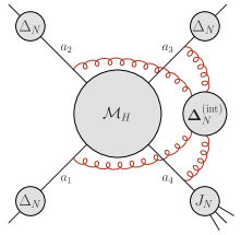
Figure 1: Pictorial representation of the all-order resummation formula in Eq. (37).

The three radiative factors $\Delta_{a_{i},N}\;(i=1,2,3)$ in the right-hand side of Eq. (37) embody soft-gluon radiation from the triggered partons $a_{1},a_{2}$ and $a_{3}$ of the partonic process in Eq. (3). The $N$-moment factor $\Delta_{a,N}$ depends on the flavour of the radiating parton $a$, on the partonic hard scale $Q^{2}$, and on the factorization scale of the corresponding parton density or fragmentation function in the hadronic cross section. We have

$$\Delta_{a,N}(Q^{2};\mu^{2})=\exp\left\{\int_{0}^{1}dz\;\frac{z^{N-1}-1}{1-z}\int_{\mu^{2}}^{(1-z)^{2}Q^{2}}\frac{dq^{2}}{q^{2}}\;A_{a}(\alpha_{\mathrm{S}}(q^{2}))\right\}\;\;,$$ (38)

where $A_{a}(\alpha_{\mathrm{S}})$ is a perturbative function,

$$A_{a}(\alpha_{\mathrm{S}})=\sum_{n=1}^{\infty}\left(\frac{\alpha_{\mathrm{S}}}{\pi}\right)^{n}A_{a}^{(n)}~{}~{},$$ (39)

whose lower-order coefficients are [2, 54]

$$A_{a}^{(1)}=C_{a}~{},~{}~{}~{}~{}~{}A_{a}^{(2)}=\frac{1}{2}C_{a}\,K~{},~{}~{}~{}~{}~{}K=C_{A}\left(\frac{67}{18}-\frac{\pi^{2}}{6}\right)-\frac{5}{9}\,n_{F}~{}~{},$$ (40)

and the third-order coefficient $A_{a}^{(3)}$ is also known [55] ($A_{a}^{(3)}$ is the coefficient of the soft part of the DGLAP splitting function $P_{aa}(z,\alpha_{\mathrm{S}})$ at ${\cal O}(\alpha_{\mathrm{S}}^{3})$).

The jet function $J_{a_{4},N_{4}}$ in Eq. (37) includes soft and collinear radiation from the parton $a_{4}$ that recoils against the observed parton $a_{3}$ in the tree-level (or, more generally, elastic scattering) process $a_{1}a_{2}\rightarrow a_{3}a_{4}$. The jet function $J_{a,N}$, which depends on the flavour of the radiating parton $a$ and on the partonic hard scale $Q^{2}$, has the following all-order form:

$$J_{a,N}(Q^{2})=\exp\left\{\int_{0}^{1}dz\;\frac{z^{N-1}-1}{1-z}\;\Big{[}\int_{(1-z)^{2}Q^{2}}^{(1-z)Q^{2}}\frac{dq^{2}}{q^{2}}A_{a}(\alpha_{\mathrm{S}}(q^{2}))+\frac{1}{2}B_{a}\left(\alpha_{\mathrm{S}}\left((1-z)Q^{2}\right)\right)\Big{]}\right\}\,,$$ (41)

where $A_{a}(\alpha_{\mathrm{S}})$ is the same perturbative function as in Eqs. (38) and (39), and the perturbative function $B_{a}(\alpha_{\mathrm{S}})$ is

$$B_{a}(\alpha_{\mathrm{S}})=\sum_{n=1}^{\infty}\left(\frac{\alpha_{\mathrm{S}}}{\pi}\right)^{n}B_{a}^{(n)}\;\;,$$ (42)

with the first-order coefficient [1, 2, 3]

$$B_{a}^{(1)}=-\gamma_{a}\;\;,$$ (43)

where $\gamma_{a}$ is the same flavour coefficient as in Eq. (22).

The values of $N_{i}$ and $Q_{i}^{2}$ $(i=1,\dots,4)$ in the argument of the radiative factors $\Delta$ and $J$ in Eq. (37) depend on $r,p_{T}^{2}$ and on the moment index $N$ of $\Sigma_{N}^{\,{\rm res}}$. The specification of this dependence involves some degree of arbitrariness (see Ref. [14]) that is compensated by a corresponding dependence in the terms ${{\mbox{\boldmath$\Delta$}}}_{N}^{\rm(int)}$ and ${\cal M}_{H}$. We use the Mellin moment values

$$N_{1}=N\,\frac{r}{1+r}\;,\quad N_{2}=N\,\frac{1}{1+r}\;,\quad N_{3}=N\;,\quad N_{4}=N\,\frac{r}{(1+r)^{2}}\;\;,$$ (44)

and the common scale

$$Q^{2}_{i}=p_{T}^{2},\quad\quad i=1,2,3,4\;\;,$$ (45)

which unambiguously specify the expressions of ${{\mbox{\boldmath$\Delta$}}}_{N}^{\rm(int)}$ and ${\cal M}_{H}$ that are presented below.

The radiative factors $\Delta_{a_{i},N_{i}}$ and $J_{a_{4},N_{4}}$ are $c$-number functions. The term $|{\cal M}_{H}\rangle$ is a colour space vector (analogously to the scattering amplitude $|{\cal M}\rangle$ in Eq. (13)) and ${{\mbox{\boldmath$\Delta$}}}^{\rm(int)}$ is a colour space operator (matrix) that acts on $|{\cal M}_{H}\rangle$. Therefore, the last factor in the right-hand side of Eq. (37) has a factorized structure in colour space, and it includes all the colour correlation effects.

The colour-space radiative factor ${{\mbox{\boldmath$\Delta$}}}_{N}^{\rm(int)}$ embodies all the quantum-interference effects that are produced by soft-gluon radiation at large angles with respect to the direction of the momenta $p_{i}$ $(i=1,\dots,4)$ of the partons in the $2\rightarrow 2$ hard scattering. Its explicit expression is [14]

$${{\mbox{\boldmath$\Delta$}}}^{\rm(int)}_{N}(r;p_{T}^{2})={{\mbox{\boldmath$V$}}}_{N}^{\,\dagger}(r;p_{T}^{2})\;{{\mbox{\boldmath$V$}}}_{N}(r;p_{T}^{2})\;\;,$$ (46)

where

$${{\mbox{\boldmath$V$}}}_{N}(r;p_{T}^{2})=P_{z}\,\exp\left\{\int_{0}^{1}dz\;\frac{z^{N-1}-1}{1-z}\,{{\mbox{\boldmath$\Gamma$}}}\left(\alpha_{\mathrm{S}}\left((1-z)^{2}p_{T}^{2}\right);r\right)\right\}\;\;.$$ (47)

The soft-gluon anomalous dimension ${{\mbox{\boldmath$\Gamma$}}}(\alpha_{\mathrm{S}};r)$ is a colour space matrix, and the operator $P_{z}$ denotes $z$-ordering in the expansion of the exponential matrix. Note that the explicit expression of $\Gamma$ can be changed by adding an imaginary $c$-number contribution. This added term in $\Gamma$ produces an overall ($c$-number) phase factor in ${{\mbox{\boldmath$V$}}}_{N}$, and its effect is cancelled by ${{\mbox{\boldmath$V$}}}_{N}^{\,\dagger}$ in the expression (46) of ${{\mbox{\boldmath$\Delta$}}}^{\rm(int)}_{N}$. Therefore, any imaginary $c$-number contribution to $\Gamma$ is harmless, since it has no effect on ${{\mbox{\boldmath$\Delta$}}}_{N}^{\rm(int)}$. The anomalous-dimension matrix ${{\mbox{\boldmath$\Gamma$}}}(\alpha_{\mathrm{S}};r)$ has the perturbative expansion

$${{\mbox{\boldmath$\Gamma$}}}(\alpha_{\mathrm{S}};r)=\frac{\alpha_{\mathrm{S}}}{\pi}\,{{\mbox{\boldmath$\Gamma$}}}^{(1)}(r)+\sum_{n=2}^{\infty}\left(\frac{\alpha_{\mathrm{S}}}{\pi}\right)^{n}{{\mbox{\boldmath$\Gamma$}}}^{(n)}(r)\;\;,$$ (48)

and the explicit expression of the first-order term is

$${{\mbox{\boldmath$\Gamma$}}}^{(1)}(r) = {\bf T}_{t}^{2}\;\ln(1+r)+{\bf T}_{u}^{2}\;\ln\frac{1+r}{r}+i\pi\;{\bf T}_{s}^{2}\;$$ (49)

$$= {\bf T}_{t}^{2}\;\Bigl{(}\ln(1+r)-i\pi\Bigr{)}+{\bf T}_{u}^{2}\;\Bigl{(}\ln\frac{1+r}{r}-i\pi\Bigr{)}+i\pi\;\sum_{i=1}^{4}C_{a_{i}}\;.$$ (50)

Note that ${{\mbox{\boldmath$\Gamma$}}}^{(1)}$ includes colour correlations, which we have explicitly expressed in terms of the colour correlation operators in Eqs. (3) and (18). Note also that ${{\mbox{\boldmath$\Gamma$}}}^{(1)}(r)$ and, more generally, ${{\mbox{\boldmath$\Gamma$}}}(\alpha_{\mathrm{S}};r)$ depend on the kinematical (angular) variable $r$, at variance with the kernels $A_{a}(\alpha_{\mathrm{S}})$ and $B_{a}(\alpha_{\mathrm{S}})$ (which are independent of the kinematics) of $\Delta_{a_{i},N_{i}}$ and $J_{a_{4},N_{4}}$ in Eqs. (38) and (41).

The amplitude $|{\cal M}_{H}\rangle$ depends on the flavour, colour and kinematical variables of the elastic scattering process $a_{1}a_{2}\rightarrow a_{3}a_{4}$ in Eq. (12), and it is independent of the Mellin moment $N$ (in practice, $|{\cal M}_{H}\rangle$ embodies the residual terms of $\Sigma_{N}^{\,{\rm res}}$ that are constant, i.e. of ${\cal O}(1)$, and not logarithmically enhanced in the limit $N\rightarrow\infty$). The colour space amplitude $|{\cal M}_{H}\rangle$ has an all-order perturbative structure that is analogous to the structure of the scattering amplitude $|{\cal M}\rangle$ in Eq. (13). We write

$$|{\cal M}_{H}\rangle=\alpha_{\mathrm{S}}(\mu_{R}^{2})\left[|{\cal M}^{(0)}\rangle+\frac{\alpha_{\mathrm{S}}(\mu_{R}^{2})}{2\pi}\;|{\cal M}^{(1)}_{H}(\mu_{R})\rangle+\sum_{n=2}^{\infty}\left(\frac{\alpha_{\mathrm{S}}(\mu_{R}^{2})}{2\pi}\right)^{n}|{\cal M}^{(n)}_{H}(\mu_{R})\rangle\right]\;\;,$$ (51)

where we have omitted the explicit reference to the parton indices $a_{1}a_{2}a_{3}a_{4}$. At the lowest order, ${\cal M}_{H}$ exactly coincides with the Born-level scattering amplitude ${\cal M}^{(0)}$ ($\,|{\cal M}^{(0)}_{H}\rangle=|{\cal M}^{(0)}\rangle$). The analogy between ${\cal M}_{H}$ and ${\cal M}$ persists at higher orders, since ${\cal M}_{H}$ also refers to the elastic scattering $a_{1}a_{2}\rightarrow a_{3}a_{4}$ and it can be regarded as the ‘hard’ (i.e., IR finite) component of the virtual contributions to the renormalized scattering amplitude ${\cal M}$. The amplitude $|{\cal M}_{H}\rangle$ is obtained from $|{\cal M}\rangle$ by removing its IR divergences and a definite amount of IR finite terms. The (IR divergent and finite) terms that are removed from $|{\cal M}\rangle$ originate from the (soft) real emission contributions to the cross section and, therefore, these terms and $|{\cal M}_{H}\rangle$ specifically depend on the one-parton inclusive cross section (i.e., $|{\cal M}_{H}\rangle$ is an observable-dependent quantity).

The first-order term ${\cal M}^{(1)}_{H}$ of ${\cal M}_{H}$ can be obtained from the results of our NLO calculation of the partonic cross section near threshold. We consider the NLO result in Eqs. (23) and (3), and we use Eq. (30) to explicitly perform the change of variables $\{s,v,w\}\rightarrow\{x_{\omega},r,p_{T}^{2}\}$. Then we can compute its $N$-moments with respect to $x_{\omega}$ and, in the limit $N\rightarrow\infty$, we compare this result with the perturbative expansion of the resummation formula in Eq. (37) up to relative ${\cal O}(\alpha_{\mathrm{S}})$. From the comparison we cross-check that the structure and the coefficients of the logarithmic terms ($\ln^{2}N$ and $\ln N$) do agree, and we can extract $|{\cal M}^{(1)}_{H}\rangle$ in explicit form. Note that the colour-space factorization form of our NLO result in Eqs. (23) and (3) is essential to obtain the amplitude $|{\cal M}^{(1)}_{H}\rangle$. The ${\cal O}(\alpha_{\mathrm{S}})$ expansion of the resummation formula (37) can also be compared with the analytic NLO result of Ref. [43]. However, the latter contains only the ‘colour-summed’ function ${\cal C}^{(1)}$ of Eq. (11) and, therefore, from the comparison we can only extract the colour-summed interference ‘$\langle{\cal M}^{(0)}|{\cal M}^{(1)}_{H}\rangle+{\rm c.c.}$’. The knowledge of the colourful amplitude $|{\cal M}^{(1)}_{H}\rangle$ (rather than ‘$\langle{\cal M}^{(0)}|{\cal M}^{(1)}_{H}\rangle+{\rm c.c.}$’) is important for QCD predictions beyond the NLO (see also Eq. (61) and related comments).

Our first-order result for the hard-virtual amplitude ${\cal M}_{H}$ is

$$|{\cal M}^{(1)}_{H}\rangle=|{\cal M}^{(1)}\rangle-{{\mbox{\boldmath$I$}}}^{(1)}_{H}\;|{\cal M}^{(0)}\rangle\;,$$ (52)

where $|{\cal M}^{(1)}\rangle$ is the full one-loop scattering amplitude in Eqs. (13) and (20), and the colour space operator ${{\mbox{\boldmath$I$}}}^{(1)}_{H}$ has the following explicit form:

$${{\mbox{\boldmath$I$}}}^{(1)}_{H} ={{\mbox{\boldmath$I$}}}^{(1)}_{\rm sing}+\frac{\pi^{2}}{4}\left({\mbox{\boldmath$T$}}_{1}^{2}+{\mbox{\boldmath$T$}}_{2}^{2}+{\mbox{\boldmath$T$}}_{3}^{2}+\frac{4}{3}{\mbox{\boldmath$T$}}_{4}^{2}\right)+\frac{1}{2}\sum_{i=1}^{3}\gamma_{a_{i}}\ln\frac{\mu_{Fi}^{2}}{p_{T}^{2}}$$

$$-\frac{1}{2}\ln(1+r)\ln\frac{1+r}{r}\left({\mbox{\boldmath$T$}}_{1}^{2}+{\mbox{\boldmath$T$}}_{2}^{2}-3{\mbox{\boldmath$T$}}_{3}^{2}+{\mbox{\boldmath$T$}}_{4}^{2}\right)$$

$$-{\mbox{\boldmath$T$}}_{t}^{2}\left(\frac{\pi^{2}}{2}+\frac{1}{2}\ln^{2}(1+r)+\ln(1+r)\ln\frac{1+r}{r}\right)$$

$$-{\mbox{\boldmath$T$}}_{u}^{2}\left(\frac{\pi^{2}}{2}+\frac{1}{2}\ln^{2}\frac{1+r}{r}+\ln(1+r)\ln\frac{1+r}{r}\right)-\frac{1}{2}K_{a_{4}}$$ (53)

$$\equiv{{\mbox{\boldmath$I$}}}^{(1)}_{\rm sing}+{{\mbox{\boldmath$I$}}}^{(1)\,{\rm fin}}_{H}\;\;,$$ (54)

where the operator ${{\mbox{\boldmath$I$}}}^{(1)}_{\rm sing}$ is defined in Eq. (21) and the flavour coefficients $K_{a}$ are given in Eq. (26). Note that Eq. (52) can be rewritten in terms of ${\cal M}^{(1)\,{\rm fin}}$ in Eq. (20) and of the IR-finite part ${{\mbox{\boldmath$I$}}}^{(1)\,{\rm fin}}_{H}$ of ${{\mbox{\boldmath$I$}}}^{(1)}_{H}$ (as defined by Eq. (54)). We have

$$|{\cal M}^{(1)}_{H}\rangle=|{\cal M}^{(1)\,{\rm fin}}\rangle-{{\mbox{\boldmath$I$}}}^{(1)\,{\rm fin}}_{H}\;|{\cal M}^{(0)}\rangle\;,$$ (55)

which explicitly shows that the one-loop hard-virtual amplitude ${\cal M}_{H}^{(1)}$ is evidently IR finite.

We note that our all-order resummed results for $\Sigma_{N}^{\,{\rm res}}$ preserve the angular symmetry (i.e. the symmetry under the exchange $t\leftrightarrow u$) of the complete (i.e. without the near-threshold approximation in Eq. (36)) partonic cross section. This symmetry corresponds to the exchange $\{r,{{\mbox{\boldmath$T$}}_{1}},\gamma_{a_{1}}\}\leftrightarrow\{1/r,{{\mbox{\boldmath$T$}}_{2}},\gamma_{a_{2}}\}$, and it is manifest in our resummed formulae (see Eqs. (37), (38), (41), (44), (49), (4)).

The expressions (38), (41) and (47) of the radiative factors $\Delta,J$ and $V$ involve the integrations of $\alpha_{\mathrm{S}}(k^{2})$ over the scale $k^{2}$ that (roughly) corresponds to the square of the relative transverse momentum of each primary parton (which radiates subsequent final-state partons) that is emitted from the Born-level process $a_{1}a_{2}\rightarrow a_{3}a_{4}$. This transverse-momentum scale is then related (through the integration over $z$) to two characteristic scales of the ‘measured’ single-particle inclusive cross section, namely the ‘soft’ scale $(1-z)^{2}p_{T}^{2}$ and the ‘collinear’ scale $(1-z)p_{T}^{2}$. The soft and collinear scales are related to the total energy and recoiling invariant mass that accompany the underlying Born-level process. The factorized structure of Eq. (37) follows [14] from general features of soft and collinear QCD radiation and, therefore, it has analogies with the structure of factorization formulae that are derived for kinematically-related processes [21, 25] by using SCET methods.

The expression (49) (or (50)) of the soft-gluon anomalous dimension ${{\mbox{\boldmath$\Gamma$}}}^{(1)}(r)$ is particularly simple, though it still depends on two colour correlation operators (as recalled in Sect. 3, this is the maximal number of linearly-independent colour correlations in the case of $2\rightarrow 2$ scattering). The dependence on colour correlations simplifies in two kinematical configurations that correspond to parton production at very small or very large rapidities (in the centre–of–mass frame of the $2\rightarrow 2$ partonic reaction). In the limit $r\rightarrow 1$, which corresponds (see Eq. (29)) to $\eta\simeq 0$ or $\theta^{*}_{13}\simeq 90^{o}$, Eq. (49) gives

$${{\mbox{\boldmath$\Gamma$}}}^{(1)}(r=1)={\bf T}_{s}^{2}\,\bigl{(}-\ln 2+i\pi\bigr{)}+\sum_{i=1}^{4}C_{a_{i}}\,\ln 2\;\;,$$ (56)

where we have used Eq. (18). We note that the expression in Eq. (56) depends on a single colour correlation operator, which is simply ${\bf T}_{s}^{2}=({\bf T}_{1}+{\bf T}_{2})^{2}$, the square of the colour charge in the $s$-channel. In the limit $r\rightarrow\infty$, which corresponds to very forward production of the parton $a_{3}$ ($\eta\rightarrow+\infty$, or $\theta^{*}_{13}\rightarrow 0$), Eq. (50) gives

$${{\mbox{\boldmath$\Gamma$}}}^{(1)}(r)\simeq{\bf T}_{t}^{2}\;\ln r\,=\,{\bf T}_{t}^{2}\;2\eta\,\simeq{\bf T}_{t}^{2}\;\ln\left(\frac{2}{\theta^{*}_{13}}\right)^{2}\;\;,\quad\quad(r\gg 1)\;,$$ (57)

and we see that ${{\mbox{\boldmath$\Gamma$}}}^{(1)}$ only depends on ${\bf T}_{t}^{2}=({\bf T}_{1}+{\bf T}_{3})^{2}$, which is the square of the colour charge exchanged in the $t$-channel. An analogous result is obtained in the case of very backward production of the parton $a_{3}$ by performing the limit $r\rightarrow 0$ ($\eta\rightarrow-\infty$, or $\theta^{*}_{23}\rightarrow 0$):

$${{\mbox{\boldmath$\Gamma$}}}^{(1)}(r)\simeq{\bf T}_{u}^{2}\;\ln\frac{1}{r}\,=\,{\bf T}_{u}^{2}\;\left(-2\eta\right)\,\simeq{\bf T}_{u}^{2}\;\ln\left(\frac{2}{\theta^{*}_{23}}\right)^{2}\;\;,\quad\quad(r\ll 1)\;.$$ (58)

The fact that a single colour correlation operator survives in the limits of Eqs. (56), (57) and (58) is not accidental, and it is a general feature of $2\rightarrow 2$ parton scattering. The result in Eq. (49) refers to a specific observable, namely, the one-particle inclusive cross section. The general form of the soft-gluon anomalous dimension at ${\cal O}(\alpha_{\mathrm{S}})$ for $2\rightarrow 2$ parton scattering can be written as [14, 47]

$${{\mbox{\boldmath$\Gamma$}}}^{(1)\,{\rm obs.}}(2\rightarrow 2)={\bf T}_{t}^{2}\;\ln\left(\frac{s}{-t}\right)+{\bf T}_{u}^{2}\;\ln\left(\frac{s}{-u}\right)+i\pi\;{\bf T}_{s}^{2}+\sum_{i=1}^{4}C_{a_{i}}\,g_{i}^{{\rm obs.}}(s,t,u)\;\;,$$ (59)

where $\{s,t,u\}$ are the Mandelstam variables of the $2\rightarrow 2$ elastic process. This expression is valid for a generic (‘global’) observable that is dominated by soft-gluon radiation in $2\rightarrow 2$ hard scattering (the expression (59) is directly obtained by specifying the $m$-parton expressions in Eqs. (21) and (27) of Ref. [14] to the case of $m=4$ hard partons). The dependence of ${{\mbox{\boldmath$\Gamma$}}}^{(1)\,{\rm obs.}}$ on the observable is entirely given by the functions $g_{i}^{{\rm obs.}}$, and it produces a $c$-number contribution (it is proportional to the Casimir coefficients $C_{a_{i}}$). The dependence of ${{\mbox{\boldmath$\Gamma$}}}^{(1)\,{\rm obs.}}$ on the colour correlation operators is instead universal (i.e., independent of the specific observable). Setting $-t=-u=s/2$ in Eq. (59), ${\bf T}_{s}^{2}$ is the sole correlation operator that appears in ${{\mbox{\boldmath$\Gamma$}}}^{(1)\,{\rm obs.}}$. Considering the limit $t\rightarrow 0$ ($u\rightarrow 0$) of Eq. (59), ${\bf T}_{t}^{2}$ (${\bf T}_{u}^{2}$) is the sole correlation operator that appears in ${{\mbox{\boldmath$\Gamma$}}}^{(1)\,{\rm obs.}}$. These are exactly the colour correlation operators that are singled out by the corresponding limits in Eqs. (56), (57) and (58).

We also note that, in the large rapidity limits of Eqs. (57) and (58), the expression of ${{\mbox{\boldmath$\Gamma$}}}^{(1)}(r)$ is especially simple: it is simply proportional to ${\bf T}_{t}^{2}$ or ${\bf T}_{u}^{2}$ (as predicted by Eq. (59)) with no additional $c$-number contributions. This simplicity is due to the scale choice $Q_{i}^{2}=p_{T}^{2}$ in Eq. (45), and it has a direct interpretation as colour coherence phenomenon. The illustration of colour coherence is particularly simple for the production at large rapidities, since we can neglect effects of ${\cal O}(1/\eta)$. In the case of very forward production ($\theta^{*}_{13}\rightarrow 0$), each of the four hard partons $a_{i}$ ($i=1,\dots,4$) radiates soft partons (interjet radiation) as an independent emitter (with intensity proportional to its colour charge ${\bf T}_{i}^{2}=C_{a_{i}}$ as in Eqs. (38) and (41)) inside a small angular region of size $\theta^{*}_{13}=\theta^{*}_{24}$ around the direction of its momentum. Soft-parton radiation at larger angles (intrajet radiation) feels the coherent action of the ‘forward emitter’ (the pair of partons $a_{1}$ and $a_{3}$, which are seen as two exactly collinear partons, i.e. as a single parton, by radiation at wide angles) and of the ‘backward emitter’ (the pair of partons $a_{2}$ and $a_{4}$). The forward and backward emitters radiate (independently) with intensity proportional to their colour charge ${\bf T}_{t}^{2}=({\bf T}_{1}+{\bf T}_{3})^{2}=({\bf T}_{2}+{\bf T}_{4})^{2}$ over the wide-angle region, which occupies the large rapidity interval of size $2\eta$: this leads to the radiation probability ${\bf T}_{t}^{2}\;2\eta$ (see Eq. (57)). This colour coherence picture corresponds to the factorization structure of Eqs. (37) in terms of the corresponding radiative factors. The absence of terms proportional to ${\bf T}_{i}^{2}=C_{a_{i}}$ in Eq. (57) implies that ${\bf\Delta}^{({\rm int})}$ exactly originates from intrajet radiation, while interjet radiation is exactly included in each of the four radiative factors $\Delta_{a_{i}}(Q_{i}^{2})$ and $J_{a_{4}}(Q_{4}^{2})$. Indeed, in the limit $\theta^{*}_{13}\rightarrow 0$ ($p_{T}\simeq p_{3}^{0}\theta^{*}_{13}$), the transverse-momentum scales $(1-z)^{2}Q_{i}^{2}=(1-z)^{2}p_{T}^{2}$ in Eq. (45) precisely correspond to radiation from $p_{i}$ up to a maximum angle $\theta_{\rm max}\simeq\theta^{*}_{13}=\theta^{*}_{24}$.

The factorized structure of $\langle{\cal M}_{H}|{{\mbox{\boldmath$\Delta$}}}^{\rm(int)}_{N}|{\cal M}_{H}\rangle$ in colour space entails colour interferences between ${{\mbox{\boldmath$\Delta$}}}^{\rm(int)}_{N}$ and $|{\cal M}_{H}\rangle$. The colour interference effects start to contribute at ${\cal O}(\alpha_{\mathrm{S}}^{2})$. The dominant logarithmic terms in ${{\mbox{\boldmath$\Delta$}}}^{\rm(int)}_{N}$ are of ${\cal O}(\alpha_{\mathrm{S}}^{n}\ln^{n}N)$, and we can consider the following approximation:

$$\langle{\cal M}_{H}|{{\mbox{\boldmath$\Delta$}}}^{\rm(int)}_{N}|{\cal M}_{H}\rangle\rightarrow\langle{\cal M}^{(0)}|{{\mbox{\boldmath$\Delta$}}}^{\rm(int)}_{N}|{\cal M}^{(0)}\rangle\times\frac{|{\cal M}_{H}|^{2}}{|{\cal M}^{(0)}|^{2}}\,+{\cal O}\left(\alpha_{\mathrm{S}}(\alpha_{\mathrm{S}}\ln N)^{n}\right)\;\;,$$ (60)

which shows that the colour interference effects can be neglected up to ${\cal O}((\alpha_{\mathrm{S}}\ln N)^{n})$. Starting from ${\cal O}\left(\alpha_{\mathrm{S}}(\alpha_{\mathrm{S}}\ln N)^{n}\right)$, the colour interference effects are relevant. In particular, $\langle{\cal M}_{H}|{{\mbox{\boldmath$\Delta$}}}^{\rm(int)}_{N}|{\cal M}_{H}\rangle$ leads to the second-order contribution

$$-\frac{1}{2}\left(\frac{\alpha_{\mathrm{S}}}{\pi}\right)^{2}\,\ln N\left\{\,2\,\langle{\cal M}^{(0)}|\left({{\mbox{\boldmath$\Gamma$}}}^{(2)}+{{\mbox{\boldmath$\Gamma$}}}^{(2)\,\dagger}\right)\,|{\cal M}^{(0)}\rangle+\left(\langle{\cal M}^{(0)}|\left({{\mbox{\boldmath$\Gamma$}}}^{(1)}+{{\mbox{\boldmath$\Gamma$}}}^{(1)\,\dagger}\right)|{\cal M}_{H}^{(1)}\rangle+{\rm c.c.}\right)\right\}$$ (61)

that is incorrectly approximated by neglecting colour interferences as in the right-hand side of Eq. (60). Using the approximation in Eq. (60), the last term in the curly bracket of Eq. (61) would be replaced by $\langle{\cal M}^{(0)}|\left({{\mbox{\boldmath$\Gamma$}}}^{(1)}+{{\mbox{\boldmath$\Gamma$}}}^{(1)\,\dagger}\right)|{\cal M}^{(0)}\rangle\left(\langle{\cal M}^{(0)}|{\cal M}_{H}^{(1)}\rangle+{\rm c.c.}\right)/|{\cal M}^{(0)}|^{2}$. The expression in Eq. (61) explicitly shows that the second-order anomalous dimension ${{\mbox{\boldmath$\Gamma$}}}^{(2)}$ contributes at the same level of logarithmic accuracy as the colour interference between ${{\mbox{\boldmath$\Gamma$}}}^{(1)}$ and $|{\cal M}_{H}^{(1)}\rangle$.

The all-order structure of Eqs. (37), (38), (41) and (47) leads to the resummation of the $\ln N$ terms in exponentiated form. In Eq. (47), exponentiation has a formal meaning, since it refers to the formal exponentiation of matrices. However, the anomalous dimension matrix ${{\mbox{\boldmath$\Gamma$}}}(\alpha_{\mathrm{S}};r)$ can be diagonalized [11, 47] in colour space. After diagonalization, the resummed radiative function $\Sigma_{N}^{\,{\rm res}}$ of Eq. (37) can be written in the customary (see, e.g., Refs. [13, 39]) exponential form

$$\Sigma_{a_{1}a_{2}\rightarrow a_{3}a_{4},N}^{\,{\rm res}}(r;p_{T}^{2},\mu_{F},\mu_{f})= \!\!\!\!\!\!\!\!\!\!\!\!\!\!\sum_{I}\;{\widetilde{C}}_{I,a_{1}a_{2}a_{3}a_{4}}(\alpha_{\mathrm{S}}(p_{T}^{2}),r;p_{T}^{2},\mu_{F},\mu_{f})$$ (62)

$$\times \!\!\exp\Bigl{\{}{\cal G}_{I,a_{1}a_{2}a_{3}a_{4}}(\alpha_{\mathrm{S}}(p_{T}^{2}),\ln N,r;p_{T}^{2},\mu_{F},\mu_{f})\Bigr{\}}+{\cal O}\left(\frac{1}{N}\right)\,,$$

where the index $I$ labels the colour space eigenstates $|I(\alpha_{\mathrm{S}};r)\rangle$ of ${{\mbox{\boldmath$\Gamma$}}}(\alpha_{\mathrm{S}};r)$, and ${\widetilde{C}}$ and ${\cal G}$ are functions (they are not colour matrices). These functions are renormalization group invariant, and their dependence on $\mu_{R}$ arises by writing $\alpha_{\mathrm{S}}(p_{T}^{2})$ as a function of $\alpha_{\mathrm{S}}(\mu_{R}^{2})$ and $\ln(p_{T}^{2}/\mu_{R}^{2})$ (as in customary perturbative calculations).

The exponent function ${\cal G}_{I}$ includes all the $\ln N$ terms, and it can consistently be expanded in LL terms of ${\cal O}(\alpha_{\mathrm{S}}^{n}\ln^{n+1}N)$, NLL terms of ${\cal O}(\alpha_{\mathrm{S}}^{n}\ln^{n}N)$, NNLL terms of ${\cal O}(\alpha_{\mathrm{S}}(\alpha_{\mathrm{S}}\ln N)^{n})$, and so forth. The function ${\widetilde{C}}_{I}$ does not depend on $N$, since it includes all the terms that are constant (i.e., of ${\cal O}(1)$) in the limit $N\rightarrow\infty$. The LL terms of ${\cal G}_{I}$ (they are actually independent of $I$) are controlled by the perturbative coefficient $A_{a}^{(1)}$ in Eq. (40). The NLL terms of ${\cal G}_{I}$ are then fully determined by $A_{a}^{(2)}$ (see Eq. (40)), $B_{a}^{(1)}$ (see Eq. (43)) and ${{\mbox{\boldmath$\Gamma$}}}^{(1)}(r)$ in Eq. (49) (or, more precisely, the eigenvalues $\Gamma^{(1)}_{I}(r)$ of ${{\mbox{\boldmath$\Gamma$}}}^{(1)}$). The Born-level contribution to the function ${\widetilde{C}}_{I}$ depends on $|\langle I|{\cal M}^{(0)}\rangle|^{2}$. The first-order term ${\widetilde{C}}_{I}^{(1)}$ of the function ${\widetilde{C}}_{I}$ depends on ‘$\langle{\cal M}^{(0)}|I\rangle\langle\,I|{\cal M}_{H}^{(1)}\rangle+{\rm c.c.}$’, and this colour interference (between $|{\cal M}^{(0)}\rangle\,,|I\rangle$ and $|{\cal M}_{H}^{(1)}\rangle$) is computable from the explicit expression of $|{\cal M}_{H}^{(1)}\rangle$ (see Eqs. (52) and (4)). Since we know ${{\mbox{\boldmath$\Gamma$}}}^{(1)}$ and $|{\cal M}_{H}^{(1)}\rangle$, the colour interference between these two terms (see Eq. (61)) is known (in the colour-diagonalized expression (62), the interference is taken into account by the correlated dependence on $I$ between ${\widetilde{C}}_{I}^{(1)}$ and $\Gamma^{(1)}_{I}$ in the exponent ${\cal G}_{I}$). Therefore, the complete explicit determination of the NNLL terms in ${\cal G}_{I}$ still requires the coefficient $A_{a}^{(3)}$ in Eq. (39) (this coefficient is known [55]), the coefficient $B_{a}^{(2)}$ in Eq. (42) and the second-order anomalous dimension ${{\mbox{\boldmath$\Gamma$}}}^{(2)}(r)$ in Eq. (48). The bulk of the contributions to ${{\mbox{\boldmath$\Gamma$}}}^{(2)}(r)$ is expected [56, 45, 14, 57] to be proportional to ${{\mbox{\boldmath$\Gamma$}}}^{(1)}(r)$ and obtained by inserting the simple rescaling (the coefficient $K$ is given in Eq. (40))

$$\alpha_{\mathrm{S}}\rightarrow\alpha_{\mathrm{S}}\left[1+\frac{\alpha_{\mathrm{S}}}{\pi}\,\frac{1}{2}\,K\right]$$ (63)

in the expression of $\Gamma$ at ${\cal O}(\alpha_{\mathrm{S}})$. The coefficient $B_{a}^{(2)}$ could be extracted from NNLL computations of related processes, such as DIS [4, 58, 59] and direct-photon production [21].

We have previously noticed that the explicit contributions of the radiative factors to the factorization formula (37) depend on the choice of the scales $Q_{i}^{2}$. The specific choice in Eq. (45) is mostly a matter of convenience (in the case of direct-photon production, for instance, the scales $Q_{i}^{2}$ can be chosen in such a way that the first-order term $\Gamma^{(1)}$ vanishes [13]) and, possibly, of closer correspondence with colour coherence features. We remark that, combining the radiative factors, the complete result for $\Sigma_{N}^{\,{\rm res}}$ is fully independent of the scales $Q_{i}^{2}$. In particular, the all-order expression in Eq. (62) and the functions ${\cal G}_{I}$ and ${\widetilde{C}}_{I}$ are fully independent of $Q_{i}^{2}$, and this independence persists after the consistent truncation at arbitrary N^kLL accuracy (and/or at arbitrary orders in $\alpha_{\mathrm{S}}$).

We also note that the exponentiated expressions (38), (41) and (47) of the radiative factors can be rewritten in a different, though eventually equivalent, form. This alternative form is obtained by the replacement

$$\int_{0}^{1}dz\;\frac{z^{N-1}-1}{1-z}\;\dots\rightarrow-\int_{0}^{1-N_{0}/N}\;\frac{dz}{1-z}\;\dots$$ (64)

where $N_{0}=e^{-\gamma_{E}}$ ($\gamma_{E}=0.5772\dots$ is the Euler number). The replacement is directly valid up to NLL accuracy [2], and it is also applicable to arbitrary logarithmic accuracy (see Ref. [6] for the related details), provided the functions $B_{a}(\alpha_{\mathrm{S}})$ and ${{\mbox{\boldmath$\Gamma$}}}(\alpha_{\mathrm{S}};r)$ are correspondingly (and properly) redefined starting from ${\cal O}(\alpha_{\mathrm{S}}^{2})$ (some non-logarithmic terms have to be reabsorbed in $M_{H}$, starting from $M_{H}^{(1)}$). We remark that this alternative representation of the radiative factors leads to the same (all-order) results for $\Sigma_{N}^{\,{\rm res}}$ and for the functions ${\cal G}_{I}$ and ${\widetilde{C}}_{I}$ in Eq. (62) (different representations can only lead to differences of ${\cal O}(1/N)$).

The results that we have presented in Sect. 3 and in this section for the unpolarized scattering reaction in Eq. (1) equally apply to processes in which one or more of the three triggered partons $a_{1},a_{2}$ and $a_{3}$ (hadrons $h_{1},h_{2}$ and $h_{3}$) are spin polarized. The relation between the unpolarized and polarized cases is technically straightforward within the process-independent formalism that we have used and explicitly worked out. Since the NLO results of Sect. 3 are embodied in the ${\cal O}(\alpha_{\mathrm{S}})$ expansion of the resummed results, we comment on polarized processes by simply referring to the results presented in this section. In particular, we only remark the technical differences that occur in the final results.

The unpolarized partonic cross section in Eq. (32) is replaced by the spin-polarized cross section, and analogous replacement applies to the factors ${\sigma}^{(0)}$ and $\Sigma$ in the right-hand side. Obviously, the Born-level factor in Eq. (33) has to be computed by replacing the spin-averaged factor $|{\overline{{\cal M}^{(0)}}|^{2}}$ with the corresponding spin-dependent factor. Note that the polarized cross section can acquire an explicit dependence on the azimuthal angle $\phi$ of the two-dimensional transverse-momentum vector of the triggered parton/hadron (for instance, this dependence occurs in the case of collisions of transversely-polarized hadrons). The structure of the all-order resummation formula (37) is unchanged in the polarized case. In particular, the soft-gluon radiative factors $\Delta_{a_{i},N_{i}}$ ($i=1,2,3$) and ${{\mbox{\boldmath$\Delta$}}}_{N}^{(\rm int)}$ in Eq. (37) are exactly the same for both the unpolarized and polarized cases. This is a consequence of spin-independence of soft-gluon radiation. The dependence on the spin polarizations may enter into the resummation formula only through the factors $J_{a_{4}}$, $|{\cal M}_{H}\rangle$ and $|{{\cal M}^{(0)}|^{2}}$ in Eq. (37). We shortly comment on this dependence.

Collinear radiation is possibly sensitive to spin and spin-polarizations. In the resummation formula (37), collinear radiation is embodied in the jet function $J_{a_{4}}$ and in ${\cal M}_{H}$ (e.g., through the collinear coefficient $K_{a_{4}}$ in Eq. (4)). These collinear contributions arise from the small-mass recoiling jet $X$ in the inclusive process of Eq. (3). Since the final-state partons in the system $X$ are inclusively summed (including the sum over their spin polarizations), the ensuing collinear contributions do not depend on the polarization of the triggered partons $a_{1},a_{2}$ and $a_{3}$. Therefore, in the resummation formula (37), the only source of spin-polarization dependence is in the hard-radiation contributions embodied in ${\cal M}_{H}$ (and in $|{\cal M}^{(0)}|^{2}$).

Throughout the paper, using the bra-ket notation $\langle\,\dots|\dots\rangle$ we have denoted the sum over colours and implicitly assumed a sum over the spin polarization states of the partons $a_{i}$ of the partonic subprocess $a_{1}a_{2}\rightarrow a_{3}a_{4}$. In the case of polarized scattering, we can simply release this implicit assumption, and the products $\langle\,\dots|\dots\rangle$ are computed by using $|{\cal M}^{(0)}\rangle$ ($|{\cal M}^{(0)}|^{2}=\langle{\cal M}^{(0)}|{\cal M}^{(0)}\rangle$) and $|{\cal M}_{H}\rangle$ at fixed spin-polarization states of one or more of the three partons $a_{1},a_{2}$ and $a_{3}$ (according to the definite polarization states of the scattering process of interest). The spin dependence of the tree-level (${\cal M}^{(0)}$) and one-loop (${\cal M}^{(1)}$) amplitudes is known [48, 49]. This directly determines the spin dependence of the one-loop hard-virtual $|{\cal M}_{H}^{(1)}\rangle$ in Eq. (52), and the ensuing spin dependence of the resummation formula (37). We simply note that the computation of radiative corrections for polarized cross sections involves customary $d$-dimensional subtleties related to spin. We refer, for instance, to variants for the $d$-dimensional treatment of the Dirac matrix $\gamma_{5}$ [60], and to the use of variants of dimensional regularization [49, 61] for treating gluon polarizations. This spin-related subtleties in the computation of the one-loop amplitude ${\cal M}^{(1)}$ have to be treated in a fully consistent manner (or, consistently related [49, 60, 61]) to avoid any ensuing mismatch in the computation of ${\cal M}_{H}^{(1)}$ according to Eq. (52). We recall that our explicit expression (4) (and, in particular, the value of the coefficient $K_{a_{4}}$ in the corresponding Eq. (26)) of the operator ${{\mbox{\boldmath$I$}}}_{H}^{(1)}$ refers to the use of the customary CDR scheme.

Soft-gluon resummation at NLL accuracy for single-hadron inclusive production in collisions of longitudinally-polarized and transversely-polarized hadrons has been performed in Ref. [40]. The resummation study of Ref. [40] deals with the rapidity-integrated cross section.

The rapidity-integrated cross section is considered in the following Sect. 4.1. Owing to the straightforward relation between our resummed formulae for the unpolarized and polarized cases (as we have just discussed), in Sect. 4.1 we limit ourselves to explicitly referring to the unpolarized case.

4.1 Cross section integrated over the rapidity

A soft-gluon resummation formula that is similar to Eq. (37) can be written in the kinematically-simpler case [13, 22, 14, 39] in which the single-particle cross section is integrated over the rapidity of the observed hadron (parton). This rapidity-integrated resummation formula can be obtained from Eq. (37).

To show the relation between these resummation formulae, we consider the hadronic cross section $d\sigma_{h_{3}}/d^{2}{\bf P}_{3T}$, which is obtained by integrating the differential cross section in Eq. (2) over the rapidity of the observed hadron $h_{3}(P_{3})$. The form of the QCD factorization formula (2) is unchanged, although the partonic cross section $p^{0}_{3}d{\hat{\sigma}}/{d^{3}{\bf p}_{3}}$ is replaced by the corresponding partonic cross section $d{\hat{\sigma}}/d^{2}{\bf p}_{T}$, which is obtained by integration of $p^{0}_{3}d{\hat{\sigma}}/{d^{3}{\bf p}_{3}}$ over the rapidity $\eta$ of the parton $a_{3}$ at fixed value of its transverse momentum ${\bf p}_{T}={\bf p}_{3T}$. By analogy with Eq. (32) we define

$$\frac{d{\hat{\sigma}}_{a_{1}a_{2}\rightarrow a_{3}}}{d^{2}{\bf p}_{T}}=\frac{1}{(4\pi s)^{2}}\,{\widetilde{\Sigma}}_{a_{1}a_{2}\rightarrow a_{3}}(x_{T};p_{T}^{2},\mu_{F},\mu_{f})\;\;,$$ (65)

where the function ${\widetilde{\Sigma}}$ is dimensionless, and the kinematical variable $x_{T}$ is the customary scaling variable

$$x_{T}=\frac{2p_{T}}{\sqrt{s}}\;\;.$$ (66)

We recall (see Eq. (29)) that the variables $x_{\omega}$ and $x_{T}$ are related through the rapidity $\eta$ by the kinematical relation

$$x_{\omega}=x_{T}\cosh\eta\;\;.$$ (67)

The dependence of the cross section on the Born-level amplitude ${\cal M}^{(0)}$ (we recall that $|{\cal M}^{(0)}|^{2}$ only depends on $r=e^{2\eta}$) is included in ${\widetilde{\Sigma}}$, so that the perturbative QCD expansion of ${\widetilde{\Sigma}}$ has the following overall normalization:

$${\widetilde{\Sigma}}_{a_{1}a_{2}\rightarrow a_{3}}(x_{T};p_{T}^{2},\mu_{F},\mu_{f})=\alpha_{\mathrm{S}}^{2}(\mu_{R}^{2})\,{\widetilde{\Sigma}}_{a_{1}a_{2}\rightarrow a_{3}}^{(0)}(x_{T})\Bigl{[}1+{\cal O}(\alpha_{\mathrm{S}}(\mu_{R}^{2}))\Bigr{]}\;\;,$$ (68)

where

$${\widetilde{\Sigma}}_{a_{1}a_{2}\rightarrow a_{3}}^{(0)}(x_{T})=\int d\eta\;\;|{\overline{{\cal M}_{a_{1}a_{2}a_{3}a_{4}}^{(0)}(r=e^{2\eta})}}|^{2}\;\delta(1-x_{T}\cosh\eta)\;\;.$$ (69)

In the case of the $p_{T}$-dependent cross section of Eq. (65), the region of partonic threshold corresponds to the limit $x_{T}\rightarrow 1$. In this limit, the higher-order radiative corrections to ${\widetilde{\Sigma}}(x_{T})$ are logarithmically enhanced: the contributions in the square bracket of Eq. (68) include terms of the type $\alpha_{\mathrm{S}}^{n}\ln^{m}(1-x_{T})$ (with $m\leq 2n$) (these terms arise from the rapidity integration of the plus-distributions of the variable $x_{\omega}$). The all-order resummation of these terms is performed in Mellin space by introducing the $N$ moments ${\widetilde{\Sigma}}_{N}$ of ${\widetilde{\Sigma}}(x_{T})$ with respect to $x_{T}$, at fixed values of $p_{T}$:

$${\widetilde{\Sigma}}_{a_{1}a_{2}\rightarrow a_{3},N}(p_{T}^{2},\mu_{F},\mu_{f})\equiv\int_{0}^{1}dx_{T}\;x_{T}^{N-1}\;{\widetilde{\Sigma}}_{a_{1}a_{2}\rightarrow a_{3}}(x_{T};p_{T}^{2},\mu_{F},\mu_{f})\;\;.$$ (70)

The $N$ moments can equivalently be defined [13, 39] with respect to $x_{T}^{2}$ (rather than $x_{T}$), and the two definitions are directly related by $N\leftrightarrow 2N$.

To relate the near-threshold behaviour of the cross sections in Eqs. (32) and (65), the main observation [13, 22, 14, 39] is that the limit $x_{T}\rightarrow 1$ kinematically forces the parton rapidity to $\eta\rightarrow 0$ (see Eq. (67)). The function ${\widetilde{\Sigma}}(x_{T})$ in Eq. (65) is obtained by the rapidity integration of Eq. (32), and we have

$${\widetilde{\Sigma}}(x_{T})=\int d\eta\;\;|{\overline{{\cal M}_{a_{1}a_{2}a_{3}a_{4}}^{(0)}(r=e^{2\eta})}}|^{2}\;\Theta(1-x_{T}\cosh\eta)\;\Sigma(x_{\omega}=x_{T}\cosh\eta,r=e^{2\eta})\;\;,$$ (71)

where we have omitted the subscript ${a_{1}a_{2}\rightarrow a_{3}}$ and the common dependence on the variables $p_{T}^{2},\mu_{F},\mu_{f}$, since they do not depend on the integration variables $\eta$ and (after Mellin transformation) $x_{T}$. In the limit $x_{T}\rightarrow 1$, considering the right-hand side of Eq. (71), the smooth (non-singular) dependence of $\Sigma(x_{\omega},r)$ on $r=e^{2\eta}$ can be approximated by setting $\eta=0$ and, thus, $r=1$ (in $N$-moment space, this approximation amounts to neglecting high-order perturbative terms of ${\cal O}(1/N)$). Then $\Sigma$ only depends on $x_{\omega}=x_{T}/x$ and this dependence enters into Eq. (71) with the typical convolution structure with respect to the variable $x=1/\cosh\eta$. This convolution structure is exactly diagonalized by considering the $N$ moments, and we directly obtain the all-order resummation formula for ${\widetilde{\Sigma}}_{a_{1}a_{2}\rightarrow a_{3},N}$:

$${\widetilde{\Sigma}}_{a_{1}a_{2}\rightarrow a_{3},N}(p_{T}^{2},\mu_{F},\mu_{f})={\widetilde{\Sigma}}_{a_{1}a_{2}\rightarrow a_{3},N}^{(0)}\left[\Sigma_{a_{1}a_{2}\rightarrow a_{3}a_{4},N}^{\,{\rm res}}(r=1;p_{T}^{2},\mu_{F},\mu_{f})+{\cal O}\left(\frac{1}{N}\right)\right]\;\;,$$ (72)

where ${\widetilde{\Sigma}}_{a_{1}a_{2}\rightarrow a_{3},N}^{(0)}$ is the $N$ moment of the Born-level term in Eq. (69).

Setting $r=1$ in our resummation formula (37) for $\Sigma_{N}^{\,{\rm res}}$, we have checked that the result in Eq. (72) is consistent with the NLL resummed results for ${\widetilde{\Sigma}}_{N}$ that are derived in Ref. [39]. In particular, since the first-order anomalous dimension ${{\mbox{\boldmath$\Gamma$}}}^{(1)}(r=1)$ at $r=1$ involves the sole colour correlation operator ${{\mbox{\boldmath$T$}}}^{2}_{s}$ (see Eq. (56)), it can be easily diagonalized in colour space (the eigenvectors $|I\rangle$ are the colour states of the irreducible representations of $SU(N_{c})$ that are formed by the $s$-channel parton pair $\{a_{1},a_{2}\}$). The NLL resummation formula of Ref. [39] is indeed directly presented in its explicitly diagonalized form (i.e., in the same form as in Eq. (62)). We note that the results in Ref. [39] neglect the colour interference between ${{\mbox{\boldmath$\Delta$}}}^{\rm(int)}_{N}$ and $|{\cal M}_{H}^{(1)}\rangle$ and (in practice) use the approximation in Eq. (60) (thus, the first-order contribution of $|{\cal M}_{H}|^{2}$ was directly extracted from the NLO results of Ref. [43]): this is a consistent approximation up to NLL accuracy. We also note a difference between Eq. (72) and the resummed expressions of Ref. [39]. The resummed factor $\Sigma_{N}^{\,{\rm res}}$ in Eq. (72) depends on the transverse momentum $p_{T}$ of the triggered parton $a_{3}$, whereas the expressions of Ref. [39] depends on $P_{3T}=x_{3}p_{T}$ of the observed hadron $h_{3}$ ($x_{3}$ is the momentum fraction of the fragmentation function $d_{a_{3}/h_{3}}$ in Eq. (2)). This difference is of ${\cal O}(1/N)$ close to the hadronic threshold, and it is an effect beyond the LL level close to the partonic threshold. The dependence of $\Sigma_{N}^{\,{\rm res}}$ on $p_{T}$ is due to QCD scaling violation, and it occurs through logarithmic terms $\ln(p_{T}^{2}/\mu^{2})=\ln(P_{3T}^{2}/x_{3}^{2}\mu^{2})$ with $\mu=\mu_{R},\mu_{F},\mu_{f}$ (see, e.g., the NLO result in Eq. (3)). These logarithmic terms appear in the resummation formula as coefficients of $\ln N$ contributions at the NLL level (and higher-order levels), and their effect is comparable to the effect produced by variations of the scales $\mu=\mu_{R},\mu_{F}$ and $\mu_{f}$.

The soft-gluon resummation formula (72) is valid to all orders. It directly expresses the soft-gluon resummation for the rapidity-integrated cross section in terms of the corresponding rapidity-dependent radiative factor $\Sigma_{N}^{\,{\rm res}}$ evaluated at $r=e^{2\eta}=1$. Our result for $|{\cal M}_{H}^{(1)}\rangle$ is a necessary information to explicitly extend the rapidity-integrated resummation formula beyond the NLL accuracy.

5 Summary

In this paper we have considered the single-particle inclusive cross section at large transverse momentum in hadronic collisions. We have studied the corresponding partonic cross section in the threshold limit in which the final-state system that recoils against the triggered parton is constrained to have a small invariant mass. In this case the accompanying QCD radiation is forced to be soft and/or collinear and the cancellation between virtual and real infrared singular contributions is unbalanced, leading to large logarithmic terms in the coefficients of the perturbative expansion. Using soft and collinear approximations of the relevant five-parton matrix elements, we have computed the general structure of these logarithmically-enhanced terms in colour space at NLO. The result of this NLO computation agrees with previous (colour summed) results in the literature, and it is presented here in a compact and process-independent form. This form is factorized in colour space and this allows us to explicitly disentangle colour interference effects. We have then discussed the structure of the logarithmically-enhanced terms beyond NLO, and we have presented the resummation formula (see Eq. (37)) that controls these contributions to the $p_{T}$-dependent cross section at fixed rapidity. The formula, which is valid at arbitrary logarithmic accuracy, is written in terms of process-independent radiative factors and of a colour-space radiative factor ${{\mbox{\boldmath$\Delta$}}}^{\rm(int)}$ that takes into account soft-gluon radiation at large angles. The radiative factor ${{\mbox{\boldmath$\Delta$}}}^{\rm(int)}$ exponentiates a colour-space anomalous dimension $\Gamma$, whose first-order term ${{\mbox{\boldmath$\Gamma$}}}^{(1)}$ is presented in explicit and simple form (see Eq. (49)). All the radiative factors are explicitly given up to NLL accuracy. Our process-independent NLO result (see Eq. (3)) agrees with the expansion of the resummation formula at the same perturbative order, and it allows us to extract the explicit form of the (IR finite) hard-virtual amplitude $|{\cal M}_{H}^{(1)}\rangle$ at relative ${\cal O}(\alpha_{\mathrm{S}})$ (see Eqs. (52) and (4)). This ingredient permits full control of the colour interferences in the evaluation of the resummation factor $\langle{\cal M}_{H}|{{\mbox{\boldmath$\Delta$}}}^{\rm(int)}|{\cal M}_{H}\rangle$ and, therefore, it paves the way to the explicit extension of the resummation formula to NNLL accuracy. These resummation results are valid for both spin-unpolarized and spin-polarized hard scattering.

In the paper we have limited ourselves to considering the single-inclusive hadronic cross section. The methods applied here can be used to study other important processes that are driven by four-parton hard scattering, such as jet and heavy-quark production.

Acknowledgements. We would like to thank Daniel de Florian and Werner Vogelsang for comments on the manuscript. This research was supported in part by the Swiss National Science Foundation (SNF) under contract 200021-144352 and by the Research Executive Agency (REA) of the European Union under the Grant Agreement number PITN-GA-2010-264564 (LHCPhenoNet).

References

- [1] G. F. Sterman, Nucl. Phys. B 281 (1987) 310.
- [2] S. Catani and L. Trentadue, Nucl. Phys. B 327 (1989) 323.
- [3] S. Catani and L. Trentadue, Nucl. Phys. B 353 (1991) 183.
- [4] A. Vogt, Phys. Lett. B 497 (2001) 228.
- [5] S. Catani, D. de Florian and M. Grazzini, JHEP 0105 (2001) 025.
- [6] S. Catani, D. de Florian, M. Grazzini and P. Nason, JHEP 0307 (2003) 028.
- [7] S. Moch and A. Vogt, Phys. Lett. B 631 (2005) 48.
- [8] E. Laenen and L. Magnea, Phys. Lett. B 632 (2006) 270.
- [9] N. Kidonakis and G. F. Sterman, Phys. Lett. B 387 (1996) 867, Nucl. Phys. B 505 (1997) 321.
- [10] R. Bonciani, S. Catani, M. L. Mangano and P. Nason, Nucl. Phys. B 529 (1998) 424 [Erratum-ibid. B 803 (2008) 234].
- [11] N. Kidonakis, G. Oderda and G. F. Sterman, Nucl. Phys. B 531 (1998) 365.
- [12] E. Laenen, G. Oderda and G. F. Sterman, Phys. Lett. B 438 (1998) 173.
- [13] S. Catani, M. L. Mangano and P. Nason, JHEP 9807 (1998) 024.
- [14] R. Bonciani, S. Catani, M. L. Mangano and P. Nason, Phys. Lett. B 575 (2003) 268.
- [15] A. V. Manohar, Phys. Rev. D 68 (2003) 114019.
- [16] A. Idilbi, X. -d. Ji and F. Yuan, Nucl. Phys. B 753 (2006) 42.
- [17] T. Becher, M. Neubert and B. D. Pecjak, JHEP 0701 (2007) 076.
- [18] T. Becher, M. Neubert and G. Xu, JHEP 0807 (2008) 030.
- [19] V. Ahrens, T. Becher, M. Neubert, and L. L. Yang, Eur. Phys. J. C 62 (2009) 333.
- [20] M. Beneke, P. Falgari and C. Schwinn, Nucl. Phys. B 828 (2010) 69.
- [21] T. Becher and M. D. Schwartz, JHEP 1002 (2010) 040.
- [22] G. F. Sterman and W. Vogelsang, JHEP 0102 (2001) 016.
- [23] P. Bolzoni, S. Forte and G. Ridolfi, Nucl. Phys. B 731 (2005) 85.
- [24] N. Kidonakis and V. Del Duca, Phys. Lett. B 480 (2000) 87.
- [25] T. Becher, C. Lorentzen and M. D. Schwartz, Phys. Rev. Lett. 108 (2012) 012001.
- [26] D. de Florian, A. Kulesza and W. Vogelsang, JHEP 0602 (2006) 047.
- [27] L. G. Almeida, G. F. Sterman and W. Vogelsang, Phys. Rev. D 78 (2008) 014008.
- [28] M. Czakon, A. Mitov and G. F. Sterman, Phys. Rev. D 80 (2009) 074017.
- [29] V. Ahrens, A. Ferroglia, M. Neubert, B. D. Pecjak and L. L. Yang, JHEP 1009 (2010) 097.
- [30] V. Ahrens, A. Ferroglia, M. Neubert, B. D. Pecjak and L. -L. Yang, JHEP 1109 (2011) 070.
- [31] W. Beenakker, T. Janssen, S. Lepoeter, M. Krämer, A. Kulesza, E. Laenen, I. Niessen, S. Thewes and T. Van Daal, report NIKHEF-2012-016 (arXiv:1304.6354 [hep-ph]).
- [32] N. Kidonakis, Phys. Rev. D 81 (2010) 054028, Phys. Rev. D 83 (2011) 091503.
- [33] H. X. Zhu, C. S. Li, J. Wang and J. J. Zhang, JHEP 1102 (2011) 099; J. Wang, C. S. Li and H. X. Zhu, Phys. Rev. D 87 (2013) 034030.
- [34] S. Catani, M. L. Mangano, P. Nason and L. Trentadue, Nucl. Phys. B 478 (1996) 273.
- [35] N. Kidonakis, G. Oderda, and G. F. Sterman, Nucl. Phys. B 525 (1998) 299.
- [36] D. de Florian and W. Vogelsang, Phys. Rev. D 76 (2007) 074031.
- [37] L. G. Almeida, G. F. Sterman and W. Vogelsang, Phys. Rev. D 80 (2009) 074016.
- [38] R. Kelley and M. D. Schwartz, Phys. Rev. D 83 (2011) 045022.
- [39] D. de Florian and W. Vogelsang, Phys. Rev. D 71 (2005) 114004.
- [40] D. de Florian, W. Vogelsang and F. Wagner, Phys. Rev. D 76 (2007) 094021, Phys. Rev. D 78 (2008) 074025.
- [41] R. K. Ellis, M. A. Furman, H. E. Haber and I. Hinchliffe, Nucl. Phys. B 173 (1980) 397.
- [42] F. Aversa, P. Chiappetta, M. Greco and J. P. Guillet, Phys. Lett. B 210 (1988) 225.
- [43] F. Aversa, P. Chiappetta, M. Greco and J. P. Guillet, Nucl. Phys. B 327 (1989) 105.
- [44] S. Catani and M. H. Seymour, Nucl. Phys. B 485 (1997) 291 [Erratum-ibid. B 510 (1998) 503].
- [45] S. Catani, Phys. Lett. B 427 (1998) 161.
- [46] R. K. Ellis and J. C. Sexton, Nucl. Phys. B 269 (1986) 445.
- [47] Y. .L. Dokshitzer and G. Marchesini, JHEP 0601 (2006) 007.
- [48] Z. Bern and D. A. Kosower, Nucl. Phys. B 379 (1992) 451.
- [49] Z. Kunszt, A. Signer and Z. Trocsanyi, Nucl. Phys. B 411 (1994) 397
- [50] W. T. Giele and E. W. N. Glover, Phys. Rev. D 46 (1992) 1980; Z. Kunszt, A. Signer and Z. Trocsanyi, Nucl. Phys. B 420 (1994) 550.
- [51] P. Aurenche, R. Baier, A. Douiri, M. Fontannaz and D. Schiff, Nucl. Phys. B 286 (1987) 553.
- [52] P. Aurenche, A. Douiri, R. Baier, M. Fontannaz and D. Schiff, Phys. Lett. B 140 (1984) 87; P. Aurenche, R. Baier, M. Fontannaz and D. Schiff, Nucl. Phys. B 297 (1988) 661.
- [53] L. E. Gordon and W. Vogelsang, Phys. Rev. D 48 (1993) 3136.
- [54] M. Cacciari and S. Catani, Nucl. Phys. B 617 (2001) 253.
- [55] S. Moch, J. A. M. Vermaseren and A. Vogt, Nucl. Phys. B 688 (2004) 101, Nucl. Phys. B 691 (2004) 129.
- [56] S. Catani, B. R. Webber and G. Marchesini, Nucl. Phys. B 349 (1991) 635.
- [57] S. M. Aybat, L. J. Dixon and G. F. Sterman, Phys. Rev. D 74 (2006) 074004
- [58] S. Moch, J. A. M. Vermaseren and A. Vogt, Nucl. Phys. B 726 (2005) 317.
- [59] G. Soar, S. Moch, J. A. M. Vermaseren and A. Vogt, Nucl. Phys. B 832 (2010) 152.
- [60] W. Vogelsang, Nucl. Phys. B 475 (1996) 47.
- [61] S. Catani, M. H. Seymour and Z. Trocsanyi, Phys. Rev. D 55 (1997) 6819.