Proton Compton scattering in a unified proton-$\Delta^{+}$ Model

Abstract

We develop a field-theoretic model for the description of proton Compton scattering in which the proton and its excited state, the $\Delta^{+}$ resonance, are described as part of one multiplet with a single Rarita-Schwinger wavefunction. In order to describe the phenomena observed, it is necessary to incorporate both minimal and non-minimal couplings. The minimal coupling reflects the fact that the $\Delta^{+}$ is a charged particle, and in this model the minimal coupling contributes also to the $\gamma N\Delta$ magnetic transition. The non-minimal couplings consist of five electromagnetic form-factors, which are accessed at fixed and vanishing momentum-transfer squared with real photons in Compton scattering experiments, therefore it is possible to extract a rather well-determined set of optimal parameters which reasonably well fit the data in the resonance region 140-450 MeV. The crucial parameter which determines the $\gamma N\Delta$ transition amplitude and therefore the height of the resonance peak is equal to $3.66\pm 0.03$, in units of $\mu_{N}$. We find that this parameter also primarily determines the contributions to magnetic polarizability in this model. In the low-energy region up to 140 MeV, we separately fit the electric and magnetic polarizabilities, while keeping the other parameters fixed and obtain values in line with previous approaches. The basic model is then extended with insights gained in the traditional approaches, namely incorporating the sigma-meson channel with the currently favored parameters, and the pion vertex corrections.

I Background and Introduction

Proton is the particle which makes up the greatest fraction of the matter in the visible universe and its properties have been extensively studied. Nevertheless it still holds some mysteries, among them the physical origin of the electric and magnetic polarizabilities, right behind the more fundamental electromagnetic properties of the proton as are the electric charge and magnetic moment. Experiments have been done since the 60’s to characterize and measure the electromagnetic properties of the proton using fixed-target Compton scattering Baranov1974 ; Zieger92 ; MacGibbon1995 ; Hunger97 ; Federspiel1991 ; Wada:1981ab . In the recent two decades, high quality proton Compton scattering data in the first $\Delta$(1232MeV) resonance region have been obtained at Saskatchewan Hallin1993 , by LEGS Collaboration Blanpied01 and at Mainz MAMI Olmos2001 ; MAMI2001 . Also, in the higher energy region where some recent good data is available due to the Hall A Collaboration at Jefferson Lab Danagoulian2007 . These most recent and precise experiments have determined the static values of the electric and magnetic polarizabilities, see for example Wright2004 ; Schumacher2005 , particularly the sign and value of the magnetic polarizability which for a long time remained shrouded in uncertainty, but see Krupina:2013dya for a new proposal for additional experiments on this. Also, high precision value was obtained for the spin-polarizability Olmos2001 ; MAMI2001 which appears in the expansion of the scattering amplitudes to the third order in momentum.

Experimentally, it is certainly also possible to measure polarization asymmetries as a function of angle and energy, for example in the last experiment done at the venerable Yerevan accelerator al:1993aa and in the first resonance region by the LEGS collaboration Blanpied:1996yh . These data can well be used to discriminate any theoretical model as a strong cross-check, once the basic parameters of the model have been well-determined.

The process in the photon low energy range up to 140 MeV is dominated by contributions due to the anomalous magnetic moment as well as the polarizabilities of the nucleon. Of these additional contributions, anomalous magnetic moments contribute to the amplitude already at the linear order while polarizability starts out at the second order, thus cross-section can grow at first quadratically and then quartically with energy. This is in contrast to the minimal coupling in QED, where the Klein-Nishina cross-section is essentially constant in the relevant energy range.

Fundamental results on scattering of light on particles of spin 1/2 with anomalous magnetic moment were obtained by Powell, Low, Gell-Mann and Goldberger, Powell1949 ; GellMann1954 ; Low1954 . Early theoretical progress was driven by the phenomenologically very successful dispersion theory approach Baldin1960 ; Hearn:1962zz ; Pfeil:1974ib ; Guiasu:1978ak ; Petrunkin1981 ; Lvov1993 ; Lvov93 ; Lvov1997 ; Lvov:1979zd ; Lvov:1980wp ; L'vov:1996xd ; Drechsel:1999rf ; Pasquini2007 , see also the latest excellent review in Schumacher2013 . This approach was supplemented by insights gained from considering pion-vertex corrections and a multitude of other improvements such as those in Feuster:1998cj ; Jenkins1992 ; Kondratyuk2001 ; Schumacher2005 ; Dattoli1977 .

On the other hand, within the purely field-theoretic chiral-Lagrangian paradigm Weinberg1978 ; Gasser1983 , the development of the promising approach of Peccei Peccei1968 ; Peccei1969 was held up by difficulties in the field theory of the spin 3/2 $\Delta^{+}$ particle. The most egregious of these pathologies had been resolved in Benmerrouche:1989uc . This better understanding of the theoretical requirements on the $\Delta$ propagator led to the paper of Pascalutsa and Scholten Pascalutsa1995 in which the first workable field-theoretical model for proton Compton scattering which incorporated the contribution of the resonance was constructed. There, it was argued that the virtual spin 1/2 degrees of freedom present in the standard propagator do play a role in the Compton scattering amplitude. As we shall see, the present work’s approach most directly descends from this model of Pascalutsa and Scholten and the subsequent recent developments in Scholten1996 ; 09053861 ; Pascalutsa:1999zz ; Lensky2010 ; McGovern:2012ew ; Lensky:2012ag ; Griesshammer:2012we ; Phillips:2012xa .

A separate development was the proposal to rid the theory of spin 3/2 particles of pathologies that stem from superluminal solutions by Ranada and Sierra in Ranada:1980yx . There, it was found that taking a Rarita-Schwinger multiplet of a physical spin 3/2 and a physical spin 1/2 particle (of different mass), would result in an acceptable wave equation even when minimally coupled to the electromagnetic field. A detailed investigation of the structure of poles in the propagator revealed that additional restrictions on the Ranada and Sierra equations result in a unitary theory with positive definite residues at the Feynman poles, taking into account the location of the pole above or below the real axis Kostas10 .

In the present paper we make use of the propagator of Kostas10 , in combination with the observation of Pascalutsa and Scholten that the spin 1/2 degrees of freedom may be due to another baryon, and propose a model where this spin 1/2 mode is interpreted as the proton, such that the proton and the $\Delta$ are together described by a single multi-component wave function of Rarita-Schwinger. $\Delta^{+}$ has the same quark constitution (uud) as the proton and is only slightly, less than 300MeV heavier than the proton. The only difference between the $\Delta^{+}$ and proton is the alignment of the spins of these quarks. In the proton, the d-quark spin is anti-aligned and makes the total proton spin $\frac{1}{2}$, while in $\Delta^{+}$ all three quarks are aligned, making $\Delta^{+}$ spin $\frac{3}{2}$. This makes it very natural to consider the possibility of a unified description, see Section II for the Lagrangian and more details.

This hypothesis confers several benefits. Low energy proton Compton scattering occurs mainly through the proton and $\Delta^{+}$ in the s- and u- channel and exchange of pions in the t-channel, see Fig. 1. $\Delta^{+}(1232{\mbox{M}eV},J^{P}=\frac{3}{2}^{+})$, the lightest baryon resonance, appears in intermediate state. Furthermore, $\Delta^{+}$ is only slightly heavier than the proton, so that this contribution is not suppressed even at the lowest energies compared with the exchange of the proton alone. In our model, because of the unified description, the s/u-channel proton and $\Delta^{+}$ contributions can be calculated simultaneously as in Fig. 1 a) and b) instead of adding up the four separate contributions.

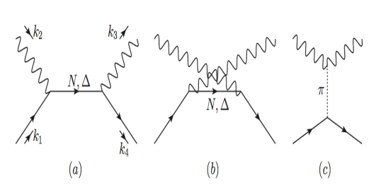
Figure 1: Tree-level Feynman diagrams for proton Compton scattering. In (a) and (b) the intermediate particle is proton or $\Delta^{+}$, and in (c) the $\pi^{0}$ meson is exchanged. (d) is the diagram for the contact interaction in (13). For appropriate photon incident energy, the intermediate $\Delta^{+}$ is approximately on-shell, and around this energy, there is the characteristic peak in the cross-section which is dominated by the $\Delta^{+}$ contribution.

The second benefit is that in this model it is possible to avoid the introduction of a large number of arbitrary parameters. In Section II.1 (see also chensav ), we present in detail the five electromagnetic form-factors which are possible for a spin 3/2 particle, these couple the momentum-independent fermion bilinears directly to the EM field strength. Three of these have clear physical interpretation as the magnetic moments of the proton and the $\Delta^{+}$, and the strength of the M1 magnetic transition between $N$ and $\Delta^{+}$. One of the remaining two parameters contributes a purely imaginary part to some amplitudes and this is disfavored by data, so that it can be safely set to zero (see Section V).

In Section III, we discuss the N-N, $\Delta^{+}$-$\Delta^{+}$, N-$\Delta^{+}$ transition matrices and derive the formulae of the proton and $\Delta^{+}$ magnetic moments. In Section IV, we calculate proton Compton scattering cross section and express electric and magnetic polarizabilites in terms of the coefficients of the non minimal interactions, and also analyze the behavior of the amplitudes around the $\Delta^{+}$ pole. We fit the Compton scattering data in Section V, and extract polarizabilities using expressions derived in Section IV. Since one linear combination of the coefficients of the non minimal interactions gives the $\Delta^{+}$ magnetic moment, our best-fit parameter set also provides a prediction of the $\Delta^{+}$ magnetic moment, but we conservatively interpret it as an upper bound. The interactions in Section II.1 can also be used to calculate the $\Delta^{+}\rightarrow N+\gamma$ decay process (Appendix A), this acts as a useful cross-check on our model.

II Lagrangian and the electromagnetic interactions

A spin 3/2 field is represented as a field with both a Lorentz index and a Dirac index. The Lagrangian in Ranada:1980yx ; Kostas10 is:

$${\mathcal{L}}=-{\bar{\psi}}_{\lambda}\,[p_{\mu}\,\Gamma^{\mu\lambda}{}_{\rho}-m\,\Theta^{\lambda}{}_{\rho}]\,\psi^{\rho},$$

$$\Gamma^{\mu\lambda}{}_{\rho}=\gamma^{\mu}\,\eta^{\lambda}{}_{\rho}+\xi\,(\gamma^{\lambda}\,\eta^{\mu}{}_{\rho}+\gamma_{\rho}\,\eta^{\lambda\mu})+\zeta\,\gamma^{\lambda}\,\gamma^{\mu}\,\gamma_{\rho},$$

$$\Theta^{\lambda}{}_{\rho}=\eta^{\lambda}{}_{\rho}-z\,\gamma^{\lambda}\,\gamma_{\rho},$$

$$\xi=2\,z-1,\ \ \ \ \zeta=6\,z^{2}-4\,z+1,$$ (1)

in which the Dirac indices are suppressed. The solutions of the corresponding wave equation are all transverse, $p_{\mu}\,\psi^{\mu}=0$, and consist of a spin 3/2 with mass m and a spin 1/2 component with mass $M=\frac{m}{6z-2}$, compared to a pure spin 3/2 field in the original Rarita-Schwinger theory. We identify the spin 3/2 and 1/2 component as $\Delta^{+}$ and proton respectively and thus unify them in one theory. This unification is very natural since proton and $\Delta^{+}$ have the same quark constituents and can transform from one into the other by absorbing or emitting a photon or even a neutral pion (which carries no charge or spin). The mass splitting between the $N$ and $\Delta$ is less than 300 MeV. The model allows to adjust the ratio of the proton to the Delta mass by choice of the $z$ parameter.

The propagator with the specific arragement of the poles is Kostas10 :

$$-iS(p) = \frac{(\not{p}+m)\,\Pi_{3}}{p^{2}-m^{2}+i\,\epsilon}-\frac{(\not{p}+M)\,\Pi_{11}}{p^{2}-M^{2}-i\,\epsilon}\,\frac{2M^{2}}{m^{2}}$$

$$+ \left[\vspace{30pt}\Pi_{22}-(\Pi_{21}+\Pi_{12})\,/B+\Pi_{11}\,3/B^{2}\right]\,\frac{3}{2\,(M+2\,m)}\leavevmode\nobreak\ \leavevmode\nobreak\ ,$$

$$B = \frac{3\,m}{2\,M+m}\leavevmode\nobreak\ \leavevmode\nobreak\ .$$ (2)

where the standard spin projection operators $\Pi$ can be found for example in Benmerrouche:1989uc .

The minimal electromagnetic interaction is usually derived by substituting $p_{\mu}\rightarrow p_{\mu}+e\,A_{\mu}$. The interaction Lagrangian is:

$${\mathcal{L}}_{I}=e\,{\bar{\psi}}_{\lambda}\,\Gamma^{\mu\lambda}{}_{\rho}\,\psi^{\rho}\,A_{\mu}\leavevmode\nobreak\ .$$ (3)

Ward identity is satisfied:

$$-i\,k_{\mu}\,\Gamma^{\mu\lambda}{}_{\rho}=S^{\lambda}{}_{\rho}(p+k)^{-1}-S^{\lambda}{}_{\rho}(p)^{-1}\leavevmode\nobreak\ ,$$ (4)

and as we shall see in the next Section there is only a finite number of additional possibilities of electromagnetic coupling which satisfy gauge invariance and the Ward identity.

II.1 Non-Minimal Electromagnetic Interactions

For phenomenological application to proton Compton scattering, minimal interaction alone does not suffice. A well known fact for Dirac theory is that it allows for two electromagnetic form factors one of which is charge and the other describes the anomalous magnetic moment. We add these as yet undetermined non-minimal interactions to the vertex:

$${\tilde{\Gamma}}^{\mu\lambda}{}_{\rho}=\Gamma^{\mu\lambda}{}_{\rho}+\frac{i}{2M}\,\sum\limits_{n}F_{n}(k^{2})\,(\Gamma_{n}{})^{\mu\lambda}{}_{\rho},$$ (5)

where the $F_{n}(k^{2})$ are form factors. If amplitudes are to be gauge invariant, the Ward identity (4) should still hold. For that, it is sufficient to set $k_{\mu}(\Gamma_{n}){}^{\mu\lambda}{}_{\rho}=0$ and thus $\Gamma_{n}$ should be of the form:

$$(\Gamma_{n})^{\mu\lambda}{}_{\rho}=(\Sigma_{n})^{\mu\nu\lambda}{}_{\rho}\,k_{\nu},$$ (6)

where $(\Sigma_{n})^{\mu\nu\lambda}{}_{\rho}$ is antisymmetric in $\mu$ and $\nu$.

Antisymmetric tensors live in the $(1,0)\oplus(0,1)$ representation of Lorentz group, and we can count the number of these representations in the product representation of the two matter fields. Representation for $\psi_{\lambda}$(or ${\bar{\psi}}_{\lambda}$) is a product of that for a vector field and that for a spinor field:

$$(\frac{1}{2},\frac{1}{2})\otimes[(\frac{1}{2},0)\oplus(0,\frac{1}{2})]=(1,\frac{1}{2})\oplus(0,\frac{1}{2})\oplus(\frac{1}{2},0)\oplus(\frac{1}{2},1).$$ (7)

The vertexes live in the tensor product of the above reducible representations, and

$$[(1,\frac{1}{2})\oplus(0,\frac{1}{2})\oplus(\frac{1}{2},0)\oplus(\frac{1}{2},1)]\otimes[(1,\frac{1}{2})\oplus(0,\frac{1}{2})\oplus(\frac{1}{2},0)\oplus(\frac{1}{2},1)]$$

$$\supset 5\ [(1,0)\oplus(0,1)]$$ (8)

This tells us there are five antisymmetric tensors and we have been able to explicitly construct them as:

$$(\Sigma_{1})^{\mu\nu\lambda}{}_{\rho}=-\frac{1}{2}\tau^{\mu\nu\lambda}{}_{\rho}\ ,$$

$$(\Sigma_{2})^{\mu\nu\lambda}{}_{\rho}=\sigma^{\mu\nu}\eta^{\lambda}{}_{\rho}\ ,$$

$$(\Sigma_{3})^{\mu\nu\lambda}{}_{\rho}=-\frac{1}{9}\gamma^{\lambda}\sigma^{\mu\nu}\gamma_{\rho}\ ,$$

$$(\Sigma_{4})^{\mu\nu\lambda}{}_{\rho}=\frac{1}{12}(\gamma^{\lambda}\gamma^{\mu}\eta^{\nu}{}_{\rho}-\gamma^{\lambda}\gamma^{\nu}\eta^{\mu}{}_{\rho}+\gamma^{\mu}\gamma_{\rho}\eta^{\nu\lambda}-\gamma^{\nu}\gamma_{\rho}\eta^{\mu\lambda})\ ,$$

$$(\Sigma_{5})^{\mu\nu\lambda}{}_{\rho}=\frac{-i}{12}(\gamma^{\lambda}\gamma^{\mu}\eta^{\nu}{}_{\rho}-\gamma^{\lambda}\gamma^{\nu}\eta^{\mu}{}_{\rho}-\gamma^{\mu}\gamma_{\rho}\eta^{\nu\lambda}+\gamma^{\nu}\gamma_{\rho}\eta^{\mu\lambda}),$$ (9)

where $\tau$ and $\sigma$ are generators of the Lorentz transformation for spin 1 and 1/2 respectively, $\tau^{\mu\nu\lambda}{}_{\rho}=i(\eta^{\mu\lambda}\eta^{\nu}{}_{\rho}-\eta^{\nu\lambda}\eta^{\mu}{}_{\rho})$ and $\sigma^{\mu\nu}=\frac{i}{4}(\gamma^{\mu}\gamma^{\nu}-\gamma^{\nu}\gamma^{\mu})$. The coefficients are normalized such that the form factors $F_{i}$ enter with equal weight in proton magnetic moment in eq.(18).

These tensors satisfy the requirement of Hermiticity:

$$[{\bar{\psi}}(p_{1})_{\lambda}\leavevmode\nobreak\ \Sigma_{i}^{\mu\nu\lambda}{}_{\rho}\leavevmode\nobreak\ \psi^{\rho}(p_{2})\leavevmode\nobreak\ (p_{1}-p_{2})_{\nu}]^{\dagger}=-{\bar{\psi}}(p_{2})_{\lambda}\leavevmode\nobreak\ \Sigma_{i}^{\mu\nu\lambda}{}_{\rho}\leavevmode\nobreak\ \psi^{\rho}(p_{1})\leavevmode\nobreak\ (p_{2}-p_{1})_{\nu},$$ (10)

which implies that the form factors $F_{i}(k^{2})$ are real.

At higher order in momenta there are a small number of additional possibilities. The pure spin 3/2 field has three form factors other than charge chensav , while only the first and second ones in eq.(9) contribute for pure spin 3/2, because $\gamma_{\rho}\,\psi^{\rho}=0$ for spin 3/2 solutions. Thus we add one more tensor:

$$(\Sigma_{6})^{\mu\nu\lambda}{}_{\rho}=\frac{1}{M^{2}}\,k^{\lambda}\,\sigma^{\mu\nu}\,k_{\rho}$$ (11)

The form factors $F_{i}(k^{2})$ which appear as coefficients in eq.(5) are scalar functions of momentum transferred squared $k^{2}=(p_{1}-p_{2})^{2}$. For real Compton scattering and Delta decay $\Delta^{+}\rightarrow p+\gamma$, the photon is on-shell $k^{2}$=0, so these form factors are taken to be constants in what follows.

II.2 Bare Polarizability Effective Lagrangian

Expanding Compton scattering cross section at low energies, static polarizabilities $\bar{\alpha}$ and $\bar{\beta}$ first enter at second order:

$$\frac{d\sigma}{d\Omega_{\mbox{\tiny lab}}}=\left(\frac{d\sigma}{d\Omega}\right)_{\mbox{\tiny Powell}}-\frac{e^{2}\omega^{2}}{4\pi M}(\frac{\bar{\alpha}+\bar{\beta}}{2}(1+\cos\theta)^{2}+\frac{\bar{\alpha}-\bar{\beta}}{2}(1-\cos\theta)^{2})+\mathcal{O}(\omega^{3}).$$ (12)

Thus, polarizabilities are here defined in the way standard in the literature, by comparing the theoretical predictions and experimental data to the Powell cross section $\left(\frac{d\sigma}{d\Omega}\right)_{\mbox{\tiny Powell}}$, which is the differential cross section of a Dirac point particle with anomalous magnetic moment included Powell1949 ; Low1954 ; GellMann1954 . A different definition would result if the Klein-Nishina result for the Dirac point particle without anomalous magnetic moment was taken as the basis for comparison. Such difference has sometimes led to confusion in the literature, but has been satisfactorily resolved by separating the contributions due to the anomalous magnetic moment. Likewise, the non-minimal interaction vertices presented in this section contribute to the effective polarizabilities $\bar{\alpha}$ and $\bar{\beta}$ as we shall see in Section IV. In addition to these vertices, we may include also the effective 4-point contact interactions that can contribute directly to the polarizabilities. Inspired by the effective Lagrangian proposed in 0611327 , we include the following interaction Lagrangian to model “bare” polarizability:

$${\cal L}_{\mbox{\tiny pol}}=\frac{i\pi}{M}\leavevmode\nobreak\ (\bar{\psi}_{\lambda}\,\Gamma^{\mu\lambda}{}_{\rho}\,\partial_{\nu}\,\psi^{\rho}-\partial_{\nu}\,\bar{\psi}_{\lambda}\,\Gamma^{\mu\lambda}{}_{\rho}\psi^{\rho})(\alpha_{B}\leavevmode\nobreak\ F_{\mu\rho}\,F^{\rho\nu}+\beta_{B}\leavevmode\nobreak\ \tilde{F}_{\mu\rho}\,\tilde{F}^{\rho\nu}).$$ (13)

This Lagrangian is not unique, but other candidates contribute identically to the cross section up to the second order in the energy of the incident photon.

The two coefficients $\alpha_{B}$ and $\beta_{B}$ we call bare polarizabilities. The contribution of this effective Lagrangian to the lab frame Compton scattering amplitudes at second order of photon energy is:

$${\cal A}_{\rm pol}=4\pi\,\alpha_{B}\,\omega\omega^{\prime}\,{\vec{\epsilon}}^{\prime}\cdot{\vec{\epsilon}}+4\pi\,\beta_{B}\,{\vec{\epsilon}}^{\prime}\times{\vec{k}}^{\prime}\cdot{\vec{\epsilon}}\times{\vec{k}}+\mathcal{O}(\omega^{3}).$$ (14)

The contribution of $\alpha_{B}$ and $\beta_{B}$ to the cross section is of the form in eq.(12). In the low energy limit where the proton is at rest before and after, and the photon frequency tends to zero, the corresponding Hamiltonian is:

$${\cal H}_{\mbox{\tiny pol}}=-2\pi(\alpha_{B}|\vec{E}|^{2}+\beta_{B}|\vec{H}|^{2}),$$ (15)

in agreement with expectations, see e.g. Lvov93 .

At higher orders in momenta it is possible to define and extract more general polarizabilities Ashley04 , such as the spin polarizabilities at cubic order.

III Magnetic Moments and the $\gamma\,N\,\Delta^{+}$ Transition Matrix

To calculate the magnetic moments, let $A^{\mu}=(0,A_{x},0,0)$ and $\vec{p}_{1}-\vec{p}_{2}=q\hat{z}$, with $\vec{p}_{1}\rightarrow 0,\vec{p}_{2}\rightarrow 0$.

$$e\,\bar{u}_{2}(p_{1},\sigma_{1})\,\tilde{\Gamma}^{\mu}\,u_{2}(p_{2},\sigma_{2})\,A_{\mu}=2\,M\,\mu_{p}\left(J_{y}^{\left(\frac{1}{2}\right)}\right)_{\sigma_{1}\sigma_{2}}(-iqA_{x})+\mathcal{O}(q^{2}),$$

$$e\,\bar{u}_{4}(p_{1},\sigma_{1})\,\tilde{\Gamma}^{\mu}\,u_{4}(p_{2},\sigma_{2})\,A_{\mu}=-2\,m\,\mu_{\Delta^{+}}\left(J_{y}^{\left(\frac{3}{2}\right)}\right)_{\sigma_{1}\sigma_{2}}(-i\,q\,A_{x})+\mathcal{O}(q^{2}).$$ (16)

In this equation, $u_{2}$ and $u_{4}$ are the spin 1/2 and spin 3/2 solutions of the wave equation and $\vec{J}^{\left(\frac{1}{2}\right)}$ and $\vec{J}^{\left(\frac{3}{2}\right)}$ are standard quantum mechanical spin operators for spin 1/2 and 3/2.

In units of $\mu_{N}=\frac{e}{2M}$ (M is proton mass), the magnetic moments of the proton and $\Delta^{+}$ as defined by eq.(16) are:

$$\frac{\mu_{p}}{\mu_{N}}=1+\lambda_{p}=1+\frac{4M(m+M)}{3m^{2}}+\frac{2M^{2}}{3m^{2}}(F_{1}+F_{2}+F_{3}+F_{5})\leavevmode\nobreak\ ,$$ (17)

$$\frac{\mu_{\Delta^{+}}}{\mu_{N}}=\frac{M}{m}+(-\frac{1}{2}F_{1}+F_{2})\leavevmode\nobreak\ .$$ (18)

When all the form factors are set to zero, $\mu_{\Delta^{+}}=\frac{e}{2m}$, so the g-factor of $\Delta^{+}$ is $\frac{2}{3}$, which agrees with expectations for that of an elementary spin 3/2 particle Belinfante:1953zz . However, even in the minimally coupled theory, the spin 1/2 particle still has an anomalous magnetic moment due to the second term in the equation (18). Proton magnetic moment $\mu_{p}\simeq 2.79$ is well measured and acts as a constraint on the form factors through eq.(18). Intriguingly, the actual value is close to that of the minimally coupled theory, so that $F_{1}+F_{2}+F_{3}+F_{5}$ is approximately zero.

$F_{6}$ does not contribute to the magnetic moments because it is higher order in the soft photon momentum k. $F_{4}$ does not enter $\mu_{\Delta^{+}}$ due to $\gamma_{\rho}\psi^{\rho}=0$ for spin 3/2 solution. Also, $F_{4}$ does not appear in the proton magnetic moment as can also be shown from the e.o.m.

In the limit of degenerate mass for proton and $\Delta^{+}$ (where in reality the mass gap is indeed small: $\frac{|m-M|}{M}\sim 0.3$), we can calculate the transition amplitudes between slowly moving proton and $\Delta^{+}$. We take $\Delta^{+}$ at rest: $p_{1}=(m,0,0,0)$ and proton momentum $p_{2}=(\sqrt{M^{2}+k^{2}},0,0,k)$ and work in the degenerate $M\rightarrow m$ limit. We take the (virtual) photon to be left polarized $A_{\tiny{L}}=\frac{1}{\sqrt{2}}(0,1,i,0)$ or right polarized $A_{\tiny{R}}=\frac{1}{\sqrt{2}}(0,1,-i,0)$ and we calculate $e\,\bar{u}_{4}\,(p_{1},\sigma_{1})\,\tilde{\Gamma}^{\mu}\,u_{2}(p_{2},\sigma_{2})\,A_{L/R\mu}$. For small $k$, the transition is $\mathcal{O}(k)$ and at first order in $k$ the result is:

$$e\leavevmode\nobreak\ \bar{u}_{4}(p_{1},\sigma_{1})\leavevmode\nobreak\ \tilde{\Gamma}^{\mu}\leavevmode\nobreak\ u_{2}(p_{2},\sigma_{2})\leavevmode\nobreak\ A_{L\mu}=e\,\frac{2}{\sqrt{3}}\,G\,k\leavevmode\nobreak\ \left(\begin{array}[]{cc}\sqrt{3}/2&0\\ 0&1/2\\ 0&0\\ 0&0\end{array}\right)_{\sigma_{1},\sigma_{2}}+\mathcal{O}(k^{2}),$$ (23)

$$e\leavevmode\nobreak\ \bar{u}_{4}(p_{1},\sigma_{1})\leavevmode\nobreak\ \tilde{\Gamma}^{\mu}\leavevmode\nobreak\ u_{2}(p_{2},\sigma_{2})\leavevmode\nobreak\ A_{R\mu}=e\,\frac{2}{\sqrt{3}}\,G\,k\leavevmode\nobreak\ \left(\begin{array}[]{cc}0&0\\ 0&0\\ -1/2&0\\ 0&-\sqrt{3}/2\end{array}\right)_{\sigma_{1},\sigma_{2}}+\mathcal{O}(k^{2}),$$ (28)

where $\tfrac{2}{\sqrt{3}}G=\frac{1}{6}\,(8+2\,F_{1}+8\,F_{2}+F_{5}-i\,F_{4})$ determines the magnetic transition amplitude between the proton and the $\Delta^{+}$. The entries of the matrix are the appropriate Clebsch-Gordan coefficients. $G$ is an important parameter and as we will see in the next Section makes the dominant contribution to the static magnetic polarizability in our model.

IV Compton Scattering Cross Section and Polarizabilities

At tree level, the Feynman diagrams for proton Compton scattering are shown in Fig.1. For s and u channels, the vertices were given in the previous section in eq.(5, 6, 9, 11).

For pion exchange t-channel diagram, there is no contribution from $\Delta^{+}$, and we use the familiar Dirac spinor for proton wave function. The relevant interaction Lagrangian is:

$${\cal L}_{\mbox{\tiny int}}=i\,g_{\pi}\,\bar{u}\,\gamma^{5}\,u\,\pi^{0}+\frac{1}{8}\,F_{\pi\gamma\gamma}\,\epsilon_{\mu\nu\rho\lambda}\,F^{\mu\nu}\,F^{\rho\lambda}\,\pi^{0}.$$ (29)

The incoming proton and photon have 4-momentum $k_{1}$ and $k_{2}$, and the outgoing proton and photon $k_{4}$ and $k_{3}$ respectively. With the above Feynman rules, the tree level amplitude is the sum of the three diagrams:

$${\mathcal{A}}_{\sigma_{1},\sigma_{4},\lambda_{2},\lambda_{3}}$$

$$= A^{\mu\nu}\epsilon_{\mu}(k_{2},\lambda_{2})\ \epsilon_{\nu}^{*}(k_{3},\lambda_{3})$$

$$= \Big{[}(ie)^{2}\ \ {\bar{u}_{2}}(k_{4},\sigma_{4})\ {\tilde{\Gamma}}^{\mu}\ (-i)S(k_{1}-k_{3})\ {\tilde{\Gamma}}^{\nu}\ u_{2}(k_{1},\sigma_{1})$$ (30)

$$+(ie)^{2}\ \ {\bar{u}_{2}}(k_{4},\sigma_{4})\ {\tilde{\Gamma}}^{\nu}\ (-i)S(k_{1}+k_{2})\ {\tilde{\Gamma}}^{\mu}\ u_{2}(k_{1},\sigma_{1})$$

$$+{\scriptstyle\frac{ig_{\pi}\,F_{\pi\gamma\gamma}}{(k_{1}-k_{4})^{2}-m_{\pi}^{2}}}\,{\bar{u}}(k_{4},\sigma_{4})\,\gamma^{5}\,u(k_{1},\sigma_{1})\,\epsilon^{\mu\nu\sigma\rho}\,k_{2\sigma}\,k_{3\rho}\Big{]}$$

$$\epsilon_{\mu}(k_{2},\lambda_{2})\ \epsilon_{\nu}^{*}(k_{3},\lambda_{3}).$$

In addition to diagrams in Fig.1, strong interactions contribute through the pion one-loop diagrams as in Fig. 2. Above the pion-production threshold, the diagram a) contributes to the imaginary part of the self-energy of $\Delta^{+}$ and determines the line-shape of the resonance. In principle, the imaginary part depends on c.m. momentum squared s, and all these diagrams should be taken into account at one-loop order McGovern:2012ew . For our purposes, we make an estimate of this effect by setting the imaginary part of $\Delta^{+}$ mass m to the observed width at the resonance, i.e. we analytically extend the above matrix element by substituting m with $(m_{0}-i\frac{\Gamma}{2})\sim(1210-50i)$MeV everywhere it appears in the matrix element. Despite modification of both the vertex and the propagator, this procedure preserves the Ward identity due to the analyticity of eq. (4) in $m$.

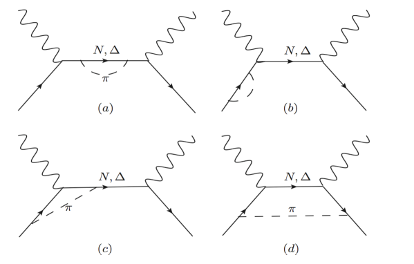
Figure 2: The one-loop level pion corrections: (a) and (b) are the self-energy diagrams; (c) and (d) are pion vertex corrections. More diagrams emerge at higher loop levels.

It is verified that our result satisfies Low’s theorem Low1954 , namely that for the low energy Compton scattering on spin 1/2 particles, the amplitudes expanded to first order of photon energy are completely determined by the mass, electric charge and magnetic moment of the spin 1/2 particle. According to the theorem, in lab frame with photon incident energy $\omega$, the amplitudes are:

$${\mathcal{A}}_{\sigma_{1},\sigma_{4},\lambda_{2},\lambda_{3}}$$

$$= \frac{e^{2}}{M}\vec{\epsilon}_{\lambda_{2}}\cdot\vec{\epsilon}^{*}_{\lambda_{3}}\delta_{\sigma_{1}\sigma_{2}}-\frac{ie\omega}{M}(2\mu_{p}-\frac{e}{2M})(\vec{\epsilon}^{*}_{\lambda_{3}}\times\vec{\epsilon}_{\lambda_{2}})\cdot\vec{\sigma}_{\sigma_{1}\sigma_{2}}$$ (31)

$$+\frac{ie\mu_{p}}{\omega M}(\vec{\epsilon}_{\lambda_{2}}\cdot\vec{k}_{3}(\vec{\epsilon}^{*}_{\lambda_{3}}\times\vec{k}_{3})-\vec{\epsilon}^{*}_{\lambda_{3}}\cdot\vec{k}_{2}(\vec{\epsilon}_{\lambda_{2}}\times\vec{k}_{2}))\cdot\vec{\sigma}_{\sigma_{1}\sigma_{2}}$$

$$+\frac{2i\mu_{p}^{2}}{\omega}((\vec{\epsilon}^{*}_{\lambda_{3}}\times\vec{k}_{3})\times(\vec{\epsilon}_{\lambda_{2}}\times\vec{k}_{2}))\cdot\vec{\sigma}_{\sigma_{1}\sigma_{2}}+O(\omega^{2}).$$

Expansion of the cross section to second order in photon energy $\omega$ is exactly in the form of eq.(12) with $\bar{\alpha}\pm\bar{\beta}$:

$$\bar{\alpha}+\bar{\beta}\sim -0.860-0.556F_{1}-1.789F_{2}-0.240F_{5}$$

$$-0.069F_{1}^{2}-0.961F_{2}^{2}-0.015F_{4}^{2}-0.020F_{5}^{2}$$

$$-0.536F_{1}F_{2}-0.023F_{1}F_{3}-0.085F_{1}F_{5}+0.009F_{2}F_{3}$$

$$-0.234F_{2}F_{5}-0.007F_{3}F_{5}+\alpha_{B}+\beta_{B}\ (10^{-4}fm^{3}),$$

$$\bar{\alpha}-\bar{\beta}\sim 1.894+1.284F_{1}+2.602F_{2}+0.202F_{3}+0.650F_{5}$$ (32)

$$+0.146F_{1}^{2}+1.339F_{2}^{2}+0.028F_{3}^{2}+0.023F_{4}^{2}+0.064F_{5}^{2}$$

$$+0.728F_{1}F_{2}+0.069F_{1}F_{3}+0.177F_{1}F_{5}+0.101F_{2}F_{3}$$

$$+0.447F_{2}F_{5}+0.067F_{3}F_{5}+\alpha_{B}-\beta_{B}\ (10^{-4}fm^{3}).$$

where $\alpha_{B}$ and $\beta_{B}$ are bare polarizabilities defined in eq.(15).

IV.1 Amplitudes at the $\Delta^{+}$ Pole

In reality, $\Delta^{+}$ and proton have small mass gap:

$$m=M(1+x-i\,y),$$ (33)

where $x\sim 0.3$ and $y\sim 0.05\sim\frac{1}{2}\,x^{2}$. And around the $\Delta^{+}$ resonance, the photon momentum q is of the same order as x, we can approximate the amplitudes to lowest non-trivial order of q, x and y.

First, at the $\Delta^{+}$ pole position, the contribution to the pole mainly comes from the first term in the propagator in s-channel where the momentum propagated is $k_{1}+k_{2}$. In this case, the denominator contributing to the pole is $(k_{1}+k_{2})^{2}-m^{2}=(E_{CM}-m)(E_{CM}+m)$. We multiply the amplitudes by $(E_{CM}-m)$ and then expand it with respect to q, x, and y. We define $q=r_{1}x$ and $y=r_{2}x^{2}$. Around the peak, $r_{1}\sim 1$ and $r_{2}\sim 0.5$. Then we can expand the amplitudes multiplied with $(E_{CM}-m)$ with respect to x, and finally set $r_{1}=1$(at the peak) and $r_{2}=\frac{y}{x^{2}}$. In center of mass frame, we rotate the proton wave functions to make it polarized along its direction of moving. That is, for proton moving in direction $\theta$ with respect to z-axis:

$$\tilde{u}_{2}(p,\frac{1}{2})=\cos\Big{(}\frac{\theta}{2}\Big{)}\leavevmode\nobreak\ u_{2}(p,\frac{1}{2})+\sin\Big{(}\frac{\theta}{2}\Big{)}\leavevmode\nobreak\ u_{2}(p,-\frac{1}{2}),$$

$$\tilde{u}_{2}(p,-\frac{1}{2})=-\sin\Big{(}\frac{\theta}{2}\Big{)}\leavevmode\nobreak\ u_{2}(p,\frac{1}{2})+\cos\Big{(}\frac{\theta}{2}\Big{)}\leavevmode\nobreak\ u_{2}(p,-\frac{1}{2}).$$ (34)

Then the approximate amplitudes are:

$${\cal A}_{ppRR}=\frac{(2ir_{2}+1-2|G|^{2})x^{2}\cos^{3}\frac{\theta}{2}}{2(E_{CM}-m)},$$

$${\cal A}_{ppRL}=\frac{(-2ir_{2}-1-2|G|^{2})x^{2}\cos\frac{\theta}{2}\sin^{2}\frac{\theta}{2}}{2(E_{CM}-m)},$$

$${\cal A}_{ppLR}=\frac{(-2ir_{2}-1-2|G|^{2})x^{2}\cos\frac{\theta}{2}\sin^{2}\frac{\theta}{2}}{2(E_{CM}-m)},$$

$${\cal A}_{ppLL}=\frac{(6ir_{2}+3+2|G|^{2}+3(2ir_{2}+1-2|G|^{2})\cos\theta)x^{2}\cos\frac{\theta}{2}}{12(E_{CM}-m)},$$

$${\cal A}_{pmRR}=\frac{(2ir_{2}+1-2|G|^{2})x^{2}\cos^{2}\frac{\theta}{2}\sin\frac{\theta}{2}}{2(E_{CM}-m)},$$

$${\cal A}_{pmRL}=\frac{(-2ir_{2}-1-2|G|^{2})x^{2}\sin^{3}\frac{\theta}{2}}{2(E_{CM}-m)},$$

$${\cal A}_{pmLR}=\frac{(-6ir_{2}-3+2|G|^{2}+3(2ir_{2}+1+2|G|^{2})\cos\theta)x^{2}\sin\frac{\theta}{2}}{12(E_{CM}-m)},$$

$${\cal A}_{pmLL}=\frac{(2ir_{2}+1-2|G|^{2})x^{2}\cos^{2}\frac{\theta}{2}\sin\frac{\theta}{2}}{2(E_{CM}-m)}.$$ (35)

In the above expressions, $x=\frac{\mbox{\tiny Re}(m)-M}{M}$, $r_{2}=\frac{y}{x^{2}}=-\frac{\mbox{\tiny Im}(m)}{Mx^{2}}$. $G$ is the combination of form factors which describes the $\gamma N\Delta^{+}$ transition amplitude as described in the previous section in eq.(28). For the subscript of the amplitudes, the first/second p/m stands for the final/initial proton polarization and the first/second L/R for final/initial photon polarization. Here only 8 of the 16 amplitudes are given, since the other 8 are related by parity:

$${\cal A}_{mmRR}={\cal A}_{ppLL},\ \ \ \ \ \ \ {\cal A}_{mpRR}=-{\cal A}_{pmLL},$$

$${\cal A}_{mmRL}={\cal A}_{ppLR},\ \ \ \ \ \ \ {\cal A}_{mpRL}=-{\cal A}_{pmLR},$$

$${\cal A}_{mmLR}={\cal A}_{ppRL},\ \ \ \ \ \ \ {\cal A}_{mpLR}=-{\cal A}_{pmRL},$$

$${\cal A}_{mmLL}={\cal A}_{ppRR},\ \ \ \ \ \ \ {\cal A}_{mpLL}=-{\cal A}_{pmRR}.$$ (36)

In the same limit, the magnetic polarizability has an approximation:

$$\bar{\beta}=-\frac{4\alpha|G|^{2}}{3xM^{3}}+\beta_{B}.$$ (37)

This may imply that the magnetic polarizability has something to do with proton-$\Delta$ (magnetic) transition.

V Fitting Data

We fit the model to the 714 proton Compton scattering datapoints from 8 experimentsHallin1993 ; Baranov1974 ; Zieger92 ; Hunger97 ; Blanpied01 ; MAMI2001 ; Olmos2001 ; MacGibbon1995 . Only data points with photon incident energy smaller 455MeV are used, in the so-called first resonance region. In principle, one can also compare the model predictions with polarized measurements, where some data is available al:1993aa ; Wada:1981ab .

For several reasons, we set $F_{4}=0$ in our fitting. First, $F_{4}$ does not enter in the expressions of proton and $\Delta^{+}$ magnetic moments eq.(18). Second, in all fits we attempted, the best fit value of $F_{4}$ was nearly exactly zero, and in any case statistically consistent with zero.

The parameters we use to fit are chosen to be $F_{1}$, $\mu\equiv\frac{\mu_{\Delta}^{+}}{\mu_{N}}=\frac{M}{m}+F_{2}-\frac{1}{2}F_{1}$, $G=\frac{1}{4\sqrt{6}}(2F_{1}+8F_{2}+F_{5}+8)$, $F_{6}$ and the bare polarizabilities $\alpha_{B}$ and $\beta_{B}$ in eq.(13). $F_{3}$ is constrained using proton magnetic moment, see eq.(18).

We minimize $\chi^{2}=\sum_{i=1}^{714}\frac{((\frac{d\sigma}{d\Omega})_{i}^{\mbox{\tiny\it calc}}-(\frac{d\sigma}{d\Omega})_{i}^{\mbox{\tiny\it data}})^{2}}{\sigma_{\mbox{\tiny(stat)}i}^{2}+\sigma_{\mbox{\tiny(syst)}i}^{2}}$. We did not attempt to rescale the data of each experiment within its own systematical uncertainty to see if it would lead to better consistency between datasets as it was done in Baranov:2000na . The optimal set of parameters was found to be: $F_{1}=-27.5$, $\mu=14.2$, $G=3.13$, $F_{6}=12.9$, $\alpha_{B}=7.5$, $\beta_{B}=-8.2$ with $\chi^{2}\sim 6.3\times 10^{3}$.

We plot the c.m. frame cross section using the above fit parameters, together with data points in Fig.3 and 4. Those data measured or recorded in lab frame have been converted to c.m. frame. From Fig.4 it is seen that the low energy cross section fit badly.

On average for each data point the fit is of $3\sigma$ deviation from the experiment value. The $\Delta^{+}$ resonance region is fitted well, while the low energy cross section deviates greatly from data points. In fact, the 68 data points with incident photon energy smaller than 140MeV out of the total 714 data points contributes nearly a third of the total $\chi^{2}$. Our fit cannot take care of the low energy ($\begin{array}[]{c}\,\vspace{-0.5em}\sim\vspace{-1.7em}\\ <\end{array}$140MeV) data points and ”high” energy ($\begin{array}[]{c}\,\vspace{-0.5em}\sim\vspace{-1.7em}\\ >\end{array}$200MeV) data points simultaneously. When giving a good fit in the resonance region, where most data points used in this paper lie in, the predicted cross section at low energy cannot account of the large asymmetry of the cross section data at forward and backward angles. Our fit cross sections at low energies are much higher than the data at forward angles and lower at backward angles. Since the polarizabilities are extracted according to low energy expansion of the cross section in eq.(12), it is expected that the predicted $\bar{\alpha}+\bar{\beta}$, calculated using eq.(32) where $F_{2}$ and $F_{5}$ are solved from the definitions of $\mu$ and $G$, is smaller than the experimental value, and $\bar{\alpha}-\bar{\beta}$ larger than experimental value. For the above fit values, $\bar{\alpha}+\bar{\beta}=-2.6(10^{-4}fm^{3})$, $\bar{\alpha}-\bar{\beta}=45.1(10^{-4}fm^{3})$. By contrast, the original experiments have quoted values extracted from the same data of $\bar{\alpha}+\bar{\beta}$ at about $14.0(10^{-4}fm^{3})$, and $\bar{\alpha}-\bar{\beta}$ at about $10.0(10^{-4}fm^{3})$.

We plot the c.m. frame cross section using the above fit parameters, together with data points in Fig.3 and 4.

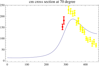
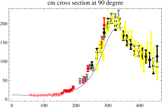
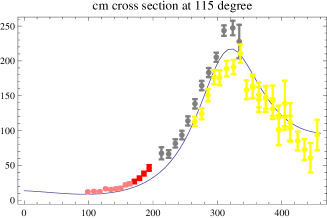
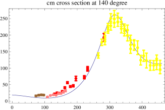
Figure 3: Fixed c.m. angle cross section and the data points, where the parameters from the fitting to all the 714 data points are used for the theoretical cross section curve. The x-axis is lab frame photon energy and y-axis is c.m. frame differential cross section in unit of nb. For Hallin1993 ; Baranov1974 ; Zieger92 ; Hunger97 ; Blanpied01 ; MAMI2001 ; Olmos2001 ; MacGibbon1995 , we use colors: Green, Blue, Black, Brown, Red, Gray, Pink and Yellow respectively. The angles of the data points included may differ from the values claimed by at most 3 degree.

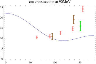
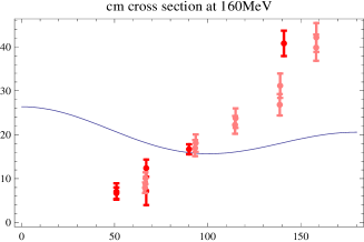
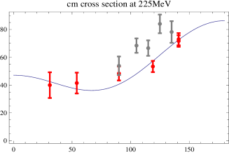
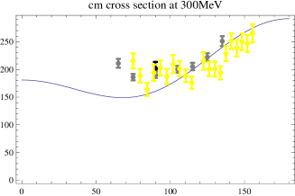
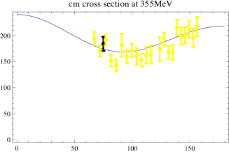
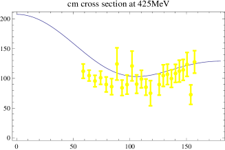
Figure 4: Fixed c.m. angle cross section and the data points, where the parameters from the fitting to all the 714 data points are used for the theoretical cross section curve. The x-axis is c.m. frame scattering angle and y-axis is c.m. frame differential cross section in unit of nb. For Hallin1993 ; Baranov1974 ; Zieger92 ; Hunger97 ; Blanpied01 ; MAMI2001 ; Olmos2001 ; MacGibbon1995 , we use colors: Green, Blue, Black, Brown, Red, Gray, Pink and Yellow respectively. The incident photon energy of the data points included may differ from the values claimed by at most 4MeV.

$\begin{array}[]{ccccc}&F_{1}&G&\mu&F_{6}\\ \raisebox{42.67912pt}{$F_{1}$}&\raisebox{42.67912pt}{$\not$}&\mbox{}\includegraphics[height=85.35826pt,width=85.35826pt]{chisquwithGF1}&\includegraphics[height=85.35826pt,width=85.35826pt]{chisquwithmuF1}&\includegraphics[height=85.35826pt,width=85.35826pt]{chisquwithF6F1}\\ \raisebox{42.67912pt}{$G$}&\includegraphics[height=85.35826pt,width=85.35826pt]{chisquwithF1G}&\raisebox{42.67912pt}{$\not$}&\includegraphics[height=85.35826pt,width=85.35826pt]{chisquwithmuG}&\includegraphics[height=85.35826pt,width=85.35826pt]{chisquwithF6G}\\ \raisebox{42.67912pt}{$\mu$}&\includegraphics[height=85.35826pt,width=85.35826pt]{chisquwithF1mu}&\includegraphics[height=85.35826pt,width=85.35826pt]{chisquwithGmu}&\raisebox{42.67912pt}{$\not$}&\includegraphics[height=85.35826pt,width=85.35826pt]{chisquwithF6mu}\\ \raisebox{42.67912pt}{$F_{6}$}&\includegraphics[height=85.35826pt,width=85.35826pt]{chisquwithF1F6}&\includegraphics[height=85.35826pt,width=85.35826pt]{chisquwithGF6}&\includegraphics[height=85.35826pt,width=85.35826pt]{chisquwithmuF6}&\raisebox{42.67912pt}{$\not$}\end{array}$

Figure 5: Projections of the 6-dimensional 95% confidence region into planes spanned by several pairs of parameters. Plots in each column share the same x-axis parameter as indicated at the top of each column. Plots in each row share the same y-axis parameter as indicated at the left of each row. Range for $F_{1}$ is (-29,-26); G: (3.1,3.25); $\mu$: (13,15); $F_{6}$: (13,17).

The challenge is clearly that the low energy part and the $\Delta^{+}$ resonance range data points is difficult to fit well at the same time. The form factors (and thus the parameters $\mu$ and $G$) are generally functions of $k^{2}$ where $k$ is photon momentum. For real Compton scattering, $k^{2}$ is always 0, so the form factors should be constants in this paper. However in the case of the bare polarizabilities it is possible that they vary with energy and/or scattering angle Schumacher2013 , which would make fitting with constant bare polarizabilities unsuccessful.

The strategy we propose to deal with the possible variation of bare polarizabilities is as follows. First, we fit only the peak range data points and fix the form factors(and $\mu$ and $G$) from this fitting. Then we fit the low energy data points varying only the bare polarizabilities. For the peak range, we use only the MAMI(2001) experiment MAMI2001 , which contains 436 data points with photon incident energy ranging from 260MeV to 455MeV. A good fit is achieved at $F_{1}=-27.7$, $G=3.17$, $\mu=14.2$, $F_{6}=14.8$, $\alpha_{B}=2.1$, $\beta_{B}=-8.1$ with $\chi^{2}\sim 830$. It is notable that $F_{1}$, $F_{6}$, $\mu$ and $G$ have not changed much from the complete fit of all data points, yet $\chi^{2}$ per datapoint is much smaller. This may be indicative of the fact that experimental data prior to this latest and more precise measurements may not be consistent with each other. In the past, one of the strategies for dealing with this has been to allow rescaling the crosssection data for each experiment within the systematical uncertainty which tends to be large Baranov:2000na .

The inclusion of the sigma channel and/or variation of the mass and width of the sigma meson do not appreciably alter the picture or the values of the best-fit parameters.

In Fig.5, we give the contour plots of $\chi^{2}$ with respect to several pairs of parameters for this fit. It is seen that $G$ is very strictly constrained.

We then use these values for $F_{1}$, $F_{6}$, $\mu$ and $G$ to fit the low energy data points, varying only $\alpha_{B}$ and $\beta_{B}$. We take 68 data points with photon incident energy below 140MeV and obtain the best fit values of $\alpha_{B}=-4.6$ and $\beta_{B}=17.9$ with $\chi^{2}\sim 194$. See Fig. 6 and 7. At these values, $\bar{\alpha}+\bar{\beta}=11.3\pm 0.9\pm 2.3(95\%C.L.)$ and $\bar{\alpha}-\bar{\beta}=7.8\pm 3.3\pm 2.0(95\%C.L.)$, much closer to values extracted (from the same data) previously. The first error is determined from the MAMI fit, by investigating how the contribution of $F_{1}$, $G$ and $\mu$ to the polarizabilities varies in the 3-dimensional 95% confidence region spanned by these three parameters. The second error is from the low energy fit.

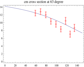
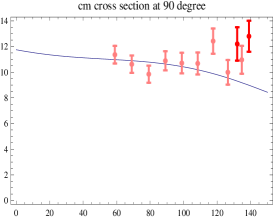
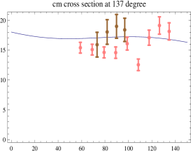
Figure 6: Fixed c.m. angle cross section and the data points with photon incident energy below 140MeV, for the fit parameters of the low energy data points. The x-axis is lab frame photon energy and y-axis is c.m. frame differential cross section in units of nanobarn. The angles of the data points included may differ from the nominal by at most 2.5 degree. For Hallin1993 ; Baranov1974 ; Zieger92 ; Hunger97 ; Blanpied01 ; MAMI2001 ; Olmos2001 ; MacGibbon1995 , we use colors: Green, Blue, Black, Brown, Red, Gray, Pink and Yellow respectively.

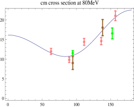
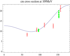
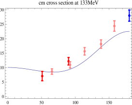
Figure 7: Fit cross section and data points with photon incident energy below 140MeV, for the fit parameters of the low energy data points. The x-axis is c.m. frame scattering angle and y-axis is c.m. frame differential cross section in units of nanobarn. The incident energy of the data points included may differ from the values claimed by at most 2.5MeV. For Hallin1993 ; Baranov1974 ; Zieger92 ; Hunger97 ; Blanpied01 ; MAMI2001 ; Olmos2001 ; MacGibbon1995 , we use colors: Green, Blue, Black, Brown, Red, Gray, Pink and Yellow respectively.

$\begin{array}[]{|c|c|c|c|c|c|c|}\hline\cr&F_{1}&G&\mu&F_{6}&\alpha_{B}&\beta_{B}\\ \hline\cr\mbox{whole fit}&-27.5&3.13&14.2&12.9&7.5&-8.2\\ \hline\cr 1\sigma&1.4&0.04&0.5&0.9&1.1&0.9\\ \hline\cr 95\%&2.8&0.08&1.1&1.7&2.2&1.6\\ \hline\cr\hline\cr\mbox{MAMI fit}&-27.7&3.17&14.2&14.8&2.1&-8.1\\ \hline\cr 1\sigma&0.7&0.03&0.4&0.8&0.8&0.5\\ \hline\cr 95\%&1.4&0.05&0.7&1.5&1.5&1.1\\ \hline\cr\hline\cr\end{array}$

$\begin{array}[]{|c|c|c|c|}\hline\cr&\mbox{value}&\mbox{95\% error from MAMI fit}&\mbox{95\% error from low energy fit}\\ \hline\cr\bar{\alpha}+\bar{\beta}&11.3&0.9&2.3\\ \hline\cr\bar{\alpha}-\bar{\beta}&7.8&3.3&2.0\\ \hline\cr\end{array}$

Table 1: Our best-fit parameter values and confidence regions

VI Discussion and Acknowledgements

Our model incorporates both minimal and non-minimal couplings. The former takes into account that the $\Delta^{+}$ is charged. The presence of the non-minimal couplings makes the description necessarily complicated, nevertheless the number of free parameters has been kept low. The parameters have clear physical interpretation, namely as the proton and $\Delta^{+}$ magnetic moment, as well as the strength of the $N\Delta$ magnetic transition (M1) and the two bare polarizabilities. We found that the data near the peak is well fit with our preferred set of parameters in the resonance region, but that the same set of parameters does not well describe the data at low energy. We have dealt with this in manner similar to McGovern:2012ew .

Although we have been able to extract a value for the $\Delta^{+}$ magnetic moment, we cannot have high confidence in this value since proton Compton scattering does not probe the $\gamma\Delta^{+}\Delta^{+}$ vertex directly. The reason that this is possible at all is that the form factors have definite properties under Lorentz transformations, so that some linear combination of parameters which affects the Compton process also determines the magnetic moment of the $\Delta^{+}$. Qualitatively, we found that changes in the $\mu_{\Delta^{+}}$ affect the predicted cross-secion asymmetrically: lower values of the magnetic moment do not drastically change the prediction, but higher values greatly enhance the crosssection, both on and off the resonance. Therefore, our result conservatively stated is that we exclude any values of the $\Delta^{+}$ magnetic moment $\mu_{\Delta^{+}}$ larger than about $14.2$. This should be compared to that extracted by MAMI Kotulla:2002cg at $2.7^{+1.0}_{-1.3}(stat)\pm 1.5(syst)\pm 3(theor)$, but note that the quoted error is dominated by theoretical model uncertainty. Our upper bound is also consistent with naive quark model expectations and some model calculations Linde:1995gr ; Kotulla:2003pm ; Kotulla:2008zz ; Kotulla:2002cg ; Kotulla:2002tx . The more reliable path towards determining the $\Delta^{+}$ magnetic moment would be to extend the model to include pion form-factors and thus cover the case of $N+\gamma\rightarrow N+\gamma+\pi$ scattering which was also very well measured by some of the very same experimental groups as the Compton data considered in the present work.

The authors would like to thank G. Georgiou and J.D. Vergados for their valuable comments.

A Project Funded by the Priority Academic Program Development of Jiangsu Higher Education Institutions (PAPD).

Appendix A $\Delta^{+}\rightarrow p+\gamma$ Decay Width

Aside from proton Compton scattering, another process can be readily accounted for in this unified $N-\Delta^{+}$ electromagnetic theory, that is the decay $\Delta^{+}\rightarrow N+\gamma$. The Feynman rules for this diagram were given in Section II.

We label the momentum and polarization of $\Delta^{+}$ as $k_{1},\sigma_{1}$, the produced photon $k_{2}$,$\lambda_{2}$ and the proton $k_{3}$,$\sigma_{3}$, the matrix element is:

$${\mathcal{A}}_{\sigma_{1},\lambda_{2},\sigma_{3}}=e\ \ {\bar{u}_{2}}(k_{3},\sigma_{3})\ {\tilde{\Gamma}}^{\mu}\ u_{4}(k_{1},\sigma_{1})\ \epsilon_{\mu}^{*}(k_{2},\lambda_{2}).$$ (38)

It is of interest to find the decay width $\Gamma_{3/2}$ and $\Gamma_{1/2}$ for the final state helicity $\frac{3}{2}$ and $\frac{1}{2}$ respectively. Evaluating this amplitude, we obtain after substituting the values of m, M:

$$\Gamma_{3/2}= 0.0047F_{1}^{2}+0.056F_{2}^{2}+0.001F_{4}^{2}+0.001F_{5}^{2}+0.032F_{1}F_{2}+0.004F_{1}F_{5}$$

$$+0.0139F_{2}F_{5}+0.032F_{1}+0.1113F_{2}+0.0139F_{5}+0.0557,$$

$$\Gamma_{1/2}= 0.0004F_{1}^{2}+0.0120F_{2}^{2}+0.0002F_{4}^{2}+0.0002F_{5}^{2}+0.0002F_{6}^{2}+0.0058F_{1}F_{2}$$ (39)

$$+0.0005F_{1}F_{5}-0.0006F_{1}F_{6}+0.0037F_{2}F_{5}-0.0039F_{2}F_{6}-0.0004F_{5}F_{6}$$

$$+0.0043F_{1}+0.0293F_{2}+0.0027F_{5}-0.0028F_{6}+0.0108.$$

If, on the other hand, we let $m=M(1+x)$ then in the limit of small x we find

$$\Gamma_{3/2}\sim\alpha Mx^{3}|G|^{2},$$

$$\Gamma_{1/2}\sim\frac{\alpha Mx^{3}|G|^{2}}{3}.$$ (40)

Experimentally $\Delta^{+}\rightarrow p+\gamma$ decay amplitudes can be extracted from the $\Delta^{+}$ peak of proton Compton scattering Blanpied01 For the MAMI fit parameters we can calculate $\Gamma_{3/2}=0.43MeV$ and $\Gamma_{1/2}=0.11MeV$, close to the values quoted in Beringer:1900zz ; Blanpied01 ; Dugger:2007bt ; Ahrens:2004pf ; Arndt:2002xv : $\Gamma_{3/2}=0.49-0.56MeV$ and $\Gamma_{1/2}=0.13-0.15MeV$.

References

- (1) P. S. Baranov, G. M. Buinov, V. G. Godin, V. A. Kuznetsova, V. A. Petrunkin, L. S. Tatarinskaya, V. S. Shirchenko and L. N. Shtarkov et al., Pisma Zh. Eksp. Teor. Fiz. 19, 777 (1974).
- (2) A. Zieger, R. Van de Vyver, D. Christmann, A. De Graeve, C. Van den Abeele and B. Ziegler, Phys. Lett. B 278, 34 (1992).
- (3) A. Hunger, J. Peise, A. Robbiano, J. Ahrens, I. Anthony, H. J. Arends, R. Beck and G. P. Capitani et al., Nucl. Phys. A 620, 385 (1997).
- (4) F. J. Federspiel, R. A. Eisenstein, M. A. Lucas, B. E. MacGibbon, K. Mellendorf, A. M. Nathan, A. O’Neill and D. P. Wells, Phys. Rev. Lett. 67, 1511 (1991).
- (5) B. E. MacGibbon, G. Garino, M. A. Lucas, A. M. Nathan, G. Feldman and B. Dolbilkin, Phys. Rev. C 52, 2097 (1995) [nucl-ex/9507001].
- (6) Y. Wada, S. Kato, T. Miyachi, K. Sugano, K. Toshioka, K. Ukai, T. Ishii and K. Egawa et al., Nuovo Cim. A 63, 57 (1981).
- (7) E. L. Hallin, D. Amendt, J. C. Bergstrom, H. S. Caplan, R. Igarashi, D. M. Skopik, E. C. Booth and D. D. Carpini et al., Phys. Rev. C 48, 1497 (1993).
- (8) G. Blanpied, M. Blecher, A. Caracappa, R. Deininger, C. Djalali, G. Giordano, K. Hicks and S. Hoblit et al., Phys. Rev. C 64, 025203 (2001).
- (9) V. Olmos de Leon, F. Wissmann, P. Achenbach, J. Ahrens, H. J. Arends, R. Beck, P. D. Harty and V. Hejny et al., Eur. Phys. J. A 10, 207 (2001).
- (10) S. Wolf, V. Lisin, R. Kondratiev, A. M. Massone, G. Galler, J. Ahrens, H. J. Arends and R. Beck et al., Eur. Phys. J. A 12, 231 (2001) [nucl-ex/0109013].
- (11) C. E. Hyde and K. de Jager, Ann. Rev. Nucl. Part. Sci. 54, 217 (2004) [nucl-ex/0507001].
- (12) M. Schumacher, Prog. Part. Nucl. Phys. 55, 567 (2005) [hep-ph/0501167].
- (13) G. Blanpied et al. [LEGS Collaboration], Phys. Rev. Lett. 76, 1023 (1996).
- (14) F. V. Adamian, A. Y. .Bunyatyan, G. S. Frangulian, P. I. Galumian, V. G. Grabsky, A. V. Airapetian, G. G. Akopian and V. K. Oktanian et al., J. Phys. G 19, L139 (1993) [J. Phys. G G 19, L139 (1993)].
- (15) A. Danagoulian et al. [Hall A Collaboration], Phys. Rev. Lett. 98, 152001 (2007) [nucl-ex/0701068 [NUCL-EX]].
- (16) J.L. Powell, Phys. Rev. 75, 32 (1949).
- (17) F. E. Low, Phys. Rev. 96, 1428 (1954).
- (18) M. Gell-Mann and M. L. Goldberger, Phys. Rev. 96, 1433 (1954).
- (19) A. C. Hearn and E. Leader, Phys. Rev. 126, 789 (1962).
- (20) W. Pfeil, H. Rollnik and S. Stankowski, Nucl. Phys. B 73, 166 (1974).
- (21) A. I. L’vov, Sov. J. Nucl. Phys. 34, 597 (1981) [Yad. Fiz. 34, 1075 (1981)].
- (22) A. I. L’vov, V. A. Petrun’kin and M. Schumacher, Phys. Rev. C 55, 359 (1997).
- (23) D. Drechsel, M. Gorchtein, B. Pasquini and M. Vanderhaeghen, Phys. Rev. C 61, 015204 (1999) [hep-ph/9904290].
- (24) A. I. L’vov, V. A. Petrunkin and S. A. Startsev, Yad. Fiz. 29, 1265 (1979).
- (25) I. Guiasu, C. Pomponiu and E. ERadescu, Annals Phys. 114, 296 (1978).
- (26) A. M. Baldin, Nucl. Phys. 18, 310 (1960).
- (27) B. Pasquini, D. Drechsel and M. Vanderhaeghen, Phys. Rev. C 76, 015203 (2007) [arXiv:0705.0282 [hep-ph]].
- (28) A. I. L’vov, Int. J. Mod. Phys. A 8, 5267 (1993).
- (29) A. I. L’vov, V. A. Petrun’kin and M. Schumacher, Phys. Rev. C 55, 359 (1997).
- (30) V. A. Petrunkin, Fiz. Elem. Chast. Atom. Yadra 12, 692 (1981).
- (31) A. I. L’vov, Phys. Lett. B 304, 29 (1993).
- (32) O. Scholten, A. Y. .Korchin, V. Pascalutsa and D. Van Neck, Phys. Lett. B 384, 13 (1996) [nucl-th/9604014].
- (33) E. E. Jenkins and A. V. Manohar, Phys. Lett. B 259, 353 (1991); A. F. Falk, Nucl. Phys. B 378, 79 (1992).
- (34) S. Kondratyuk and O. Scholten, Phys. Rev. C 64, 024005 (2001) [nucl-th/0103006].
- (35) G. Dattoli, G. Matone and D. Prosperi, Lett. Nuovo Cim. 19, 601 (1977).
- (36) V. Lensky and V. Pascalutsa, PoS EFT 09, 033 (2009) [arXiv:0905.3861 [nucl-th]].
- (37) T. Feuster and U. Mosel, Phys. Rev. C 59, 460 (1999) [nucl-th/9803057].
- (38) M. Schumacher and M. D. Scadron, arXiv:1301.1567 [hep-ph].
- (39) S. Weinberg, Physica A 96, 327 (1979).
- (40) J. Gasser and H. Leutwyler, Annals Phys. 158, 142 (1984).
- (41) R. D. Peccei, Phys. Rev. 176, 1812 (1968).
- (42) R. D. Peccei, Phys. Rev. 181, 1902 (1969).
- (43) M. Benmerrouche, R. M. Davidson and N. C. Mukhopadhyay, Phys. Rev. C 39, 2339 (1989).
- (44) V. Pascalutsa and O. Scholten, Nucl. Phys. A 591, 658 (1995).
- (45) V. Pascalutsa and R. Timmermans, Phys. Rev. C 60, 042201(R) (1999) [arXiv:nucl-th/9905065].
- (46) V. Lensky and V. Pascalutsa, Eur. Phys. J. C 65, 195 (2010) [arXiv:0907.0451 [hep-ph]].
- (47) J. A. McGovern, D. R. Phillips and H. W. Griesshammer, Eur. Phys. J. A 49, 12 (2013) [arXiv:1210.4104 [nucl-th]].
- (48) A. F. Ranada and G. Sierra, Phys. Rev. D 22, 2416 (1980).
- (49) K. G. Savvidy, arXiv:1005.3455 [hep-th].
- (50) A. Ilyichev, S. Lukashevich and N. Maksimenko, hep-ph/0611327.
- (51) G. Chen and K. G. Savvidy, Eur. Phys. J. C 72, 1952 (2012) [arXiv:1105.3851 [hep-th]].
- (52) F. J. Belinfante, Phys. Rev. 92, 997 (1953).
- (53) P. S. Baranov, A. I. L’vov, V. A. Petrun’kin and L. N. Shtarkov, nucl-ex/0011015.
- (54) J. D. Ashley, D. B. Leinweber, A. W. Thomas and R. D. Young, Eur. Phys. J. A 19, 9 (2004) [hep-lat/0308024].
- (55) M. Kotulla [TAPS/A2 Collaboration], Prog. Part. Nucl. Phys. 50, 295 (2003).
- (56) J. Linde and H. Snellman, Phys. Rev. D 53, 2337 (1996) [hep-ph/9510381].
- (57) M. Kotulla, Prog. Part. Nucl. Phys. 61, 147 (2008).
- (58) M. Kotulla, J. Ahrens, J. R. M. Annand, R. Beck, G. Caselotti, L. S. Fog, D. Hornidge and S. Janssen et al., Phys. Rev. Lett. 89, 272001 (2002) [nucl-ex/0210040].
- (59) M. Kotulla [TAPS and A2 Collaboration], Acta Phys. Polon. B 33, 957 (2002).
- (60) J. Beringer et al. [Particle Data Group Collaboration], Phys. Rev. D 86, 010001 (2012).
- (61) M. Dugger, B. G. Ritchie, J. P. Ball, P. Collins, E. Pasyuk, R. A. Arndt, W. J. Briscoe and I. I. Strakovsky et al., Phys. Rev. C 76, 025211 (2007) [arXiv:0705.0816 [hep-ex]].
- (62) J. Ahrens et al. [GDH and A2 Collaboration], Eur. Phys. J. A 21, 323 (2004).
- (63) R. A. Arndt, W. J. Briscoe, I. I. Strakovsky and R. L. Workman, Phys. Rev. C 66, 055213 (2002) [nucl-th/0205067].
- (64) T. R. Hemmert, B. R. Holstein and J. Kambor, Phys. Rev. D 55, 5598 (1997) [hep-ph/9612374].
- (65) T. R. Hemmert, B. R. Holstein, G. Knochlein and S. Scherer, Phys. Rev. Lett. 79, 22 (1997) [nucl-th/9705025].
- (66) T. R. Hemmert, B. R. Holstein, J. Kambor and G. Knochlein, Phys. Rev. D 57, 5746 (1998) [nucl-th/9709063].
- (67) R. Weiner and W. Weise, Phys. Lett. B 159, 85 (1985).
- (68) D. Babusci, G. Giordano, A. I. L’vov, G. Matone and A. M. Nathan, Phys. Rev. C 58, 1013 (1998) [hep-ph/9803347].
- (69) V. Pascalutsa, M. Vanderhaeghen and S. N. Yang, Phys. Rept. 437, 125 (2007), [arXiv:hep-ph/0609004].
- (70) D. R. Phillips, J. A. McGovern and H. W. Griesshammer, arXiv:1210.3577 [nucl-th].
- (71) H. W. Griesshammer, J. A. McGovern, D. R. Phillips and G. Feldman, Prog. Part. Nucl. Phys. 67, 841 (2012) [arXiv:1203.6834 [nucl-th]].
- (72) V. Lensky, J. A. McGovern, D. R. Phillips and V. Pascalutsa, Phys. Rev. C 86, 048201 (2012) [arXiv:1208.4559 [nucl-th]].
- (73) N. Krupina and V. Pascalutsa, arXiv:1304.7404 [nucl-th].