A framework for the calibration of social simulation models

Abstract

Simulation with agent-based models is increasingly used in the study of complex socio-technical systems and in social simulation in general. This paradigm offers a number of attractive features, namely the possibility of modeling emergent phenomena within large populations. As a consequence, often the quantity in need of calibration may be a distribution over the population whose relation with the parameters of the model is analytically intractable. Nevertheless, we can simulate. In this paper we present a simulation-based framework for the calibration of agent-based models with distributional output based on indirect inference. We illustrate our method step by step on a model of norm emergence in an online community of peer production, using data from three large Wikipedia communities. Model fit and diagnostics are discussed.

1 Introduction

Computational agent-based models (abm) are increasingly used in several areas of science because of a number of attractive features [10]. They are an effective alternative to more traditional methods because they let one test in silico different hypotheses about the origin of collective phenomena, and to explore the connection between the micro and macro levels, i.e. what kind of macroscopic patterns are generated starting from a set of microscopic interactions between agents. [25].

Like most models, abms contain tunable parameters and thus, as a first step towards empirical investigation, it is desirable to calibrate them. However, often it is not possible to formulate an equivalent analytical model, and even if this is the case, it may still be intractable or too complicated, for example when latent variables are used. In all these cases, an abm can be just regarded as a black box, and be calibrated via simulation, using the machinery developed for complex computer codes [62]. These approaches typically involve the use of emulators such as splines, polynomials, or semi-parametric techniques such as Gaussian Processes [62]. Other approaches to calibration that are not simulation-based but still use Gaussian processes are Bayesian techniques [43, 40, 6]; they have been applied in biology [20] and cosmology [39], to cite a few. Computational approaches for the calibration of abms have been developed in biology [24, 20] and economics [8, 31, 70]. Comparatively, issues related to calibration and empirical testing are still largely underrepresented in the social-simulation literature [66].

Agent-based models, though, present another difficulty to the above approaches: it is often the case that the output of an abm is a distribution of values over a population of agents, and not just a scalar or vector-valued quantity. This is common, for example, in models of social collective phenomena. Sometimes distributions can be summarized by their moments and thus methods like the Simulated Method of Moments may be applied [49]. Some other times the distribution moments do not provide a good description of the output distribution, and other approaches must be used [8, 20, 24].

In this paper we present a step-by-step data-driven methodology for calibrating an agent-based model with distributional output. We use a computational technique inspired by the indirect inference methodology [32]. This technique predicates the use of an auxiliary model to match empirical data with synthetic simulations.

Indirect inference is used to fit models to empirical data when maximum likelihood estimation is either unfeasible, or simply too complicated from a computational point of view. Examples from econometrics – where the technique first originated – include dynamical models with latent variables (cf. [32, 64]), agent-based models [8], and also dynamic models from population biology [42, 71]. A different, related approach based on simulation is the one by Gilli and Winker [31].

We apply our technique to the calibration of a model of a techno-social system, specifically a model of norm formation in an online community of social production or commons-based peer production (shortened as “peer production” in the remainder of the text) [16].

Norms are shared expectations about behaviors that members of a social group ought follow or else incur in the risk of being sanctioned by other members [54]. Norms are regarded as one of the main determinants of social behavior, a sort of grammar for social interactions [9], and are central to the understanding of group dynamics [26]. The emergence of social norms has been the subject of a long-standing tradition of investigation [36, 37, 55] and, more recently, also by means of agent-based models [2, 9, 1]. Norms may emerge from imposition from a higher authority [54], but often – and this is the case we are interested in with this paper – norms can emerge informally from the aggregated behavior of many different actors [2, 9].

Social norms are important determinants of behavior in online peer production groups, where members engage, often for free [46], in the production of digital contents [7]. In these settings users may be encouraged to contribute to the digital common by a variety of extrinsic rewards, from reputation gains [18] to simple forms of acknowledgment [15]. Furthermore, direct surveys show that the array of intrinsic motivations for contributing is surprisingly varied [58].

However, in many cases neither rewards nor personal motivations can foster true, long-term commitment to the community without the construction of a shared sense of membership [60]. This can be construed in terms of social identity [67] and self-categorization [68]. As a result, a strong, shared identity may develop, even despite the fact that interactions on the Web are often asynchronous and anonymous. For example, recent work by Neff et al. analyzed the discourse of editors from the English Wikipedia and discovered that the ‘Wikipedian’ identity can be stronger than affiliation to the two major parties of the US political system [53].

A peculiarity of peer-production groups is that norms may also specifically regulate how, and under which conditions, users contribute to the digital common. An example of a social production norm is the Neutral Point of View (npov) policy of Wikipedia. This policy prescribes users “to provide complete information, and not to promote one particular point of view over another” when contributing to encyclopedic articles. Users who do not frame their contributions following the npov guidelines are sanctioned by other peers by having their contributions rejected. Thus, besides the low barriers to contribution [18], the emergence of the proper, efficient social production norms are fundamental to the success of an online community of peer production as much as for any social group [26]. An example of this is the establishment of a “good-faith” collaboration culture in Wikipedia given by Reagle [59].

On the other hand, certain peculiar characteristics of online peer-production groups pose challenges to the study of the emergence of social norms. Mass collaboration platforms akin to Wikipedia may reach considerable sizes, and the churn among users can become surprisingly large, meaning that previous research, predicated on small group sizes and consistent participation [33], is difficult to apply.

Simple microscopic models of collective behavior are able to account for striking regularities in social phenomena, a classic example being the case of elections [29]. The model we propose in this paper addresses all the above problems by embedding a process of belief adjustment based on homophily [50] within a dynamic population [23, 38]. Social production norms emerge informally from the microscopic interactions between agents and the digital common, which in our case will be a set of pages, or artifacts. Thus our model falls within the category of norm-emergence models with structured interactions [1].

Unlike the other models of norm emergence cited so far, linking the process of norm emergence with the population dynamic gives the possibility to study the emergence of norms in a more realistic setting and, as a collateral benefit, to test it against empirical data about user participation, such as the span of user activity. We use indirect inference and our model to analyze data on user activity from three large Wikipedia communities (French, Italian, and Portuguese).

Because our objective for this paper is mainly to illustrate an abm calibration methodology, it would have seemed more sensible to set aside the problem of norm emergence in peer production groups and to focus instead on a well-established model from the literature on social simulation, such as the Schelling segregation model [63] or the Axelrod model of cultural evolution [3], to cite a few. Classic models have the advantage of a clear, extensively studied phenomenology, and usually possess few parameters, making them an effective choice for illustrative purposes. On the other hand, they are often very idealized and sometimes fail at reproducing simple empirical evidence.

Finally, the choice of studying norm emergence in an online setting can be further motivated considering that studying norm emergence in an online setting addresses a classic problem with modeling social norms and human behavior in general: while data about preferences of social actors can be collected via experimentation both online and offline [9, 11], large-scale online groups still present several problems with respect to this task. In contrast, data about social interactions in said groups are nowadays comparatively much easier to obtain, as abundant traces of human activities are readily available on the Internet [45].

The model we use here is a modification of the original model by [16], that employed homogeneous Poisson processes to describe the patterns of temporal activation of agents – an assumption that is not in line with recent findings on human activity on the Internet [57]. We found that this assumption has a profound impact on the resulting distribution of user lifespans, which makes the model not amenable for calibration against empirical data. We thus decided to lift the homogeneity assumption and introduce a realistic sub-model of temporal activation of users based on Poissonian cascades [47].

The rest of the paper is organized as follows: in section 2 we describe the collection and preparation of the user activity span data; in section 3 we describe the model of norm emergence in a community of peer production; section 4 illustrates the calibration technique in detail; section 5 gives the results of the calibration, including various diagnostics procedures. We critically evaluate the results of the calibration and conclude in section 6 and finally conclude (sec. 7).

2 Data

We measure the period of participation of a user within an online group as the span between the first and the last contribution she makes. We call this measure the user activity lifespan $\tau$. Previous research on peer-production systems shows that the period of activity of users in blogs, wikis, etc. follows a multimodal distribution [34, 17, 72, 73]. Data on user activity lifespans of Wikipedia users were obtained from the official database dumps released by the Wikimedia Foundation. We used the 2009 stub-meta-history dumps, which contain only the metadata of the revisions.

We selected the top five languages in terms of authored articles, which, as of data collection time, were English (3,7M articles as of September 2011), German (1,3M), French (1,1M), Italian (850K), and Portuguese (700K). In terms of activity lifespan they represent roughly two distinct classes, depending on the ratio between short-term and long-term users. One class, which comprises Portuguese and English, has a more even ratio than the other (French, Italian and German) [17]. The question of whether these two classes of user activity lifespan are representative of the whole catalog of Wikipedia communities is still an open one.

While we initially collected data from these five different Wikipedia communities, computational issues with the English and the German wikis eventually forced us to drop these two, which were the most populated and thus could not be simulated in a reasonable amount of time (i.e., they required $>1$ month), given our limited resources. Because each community is simulated independently of the others, exclusion of these two dataset does not impact the results about the other three. It also leaves us with at least one specimen per activity lifespan class. We thus decided to report results only from the remaining three: French, Italian, and Portuguese. For a histogram of the lifespan data, see Figure 6.

The raw data from the dumps includes details about each revision to a Wikipedia article, the time stamp, user id, user name, and additional information. As an example of the raw data format, Table 1 reports five consecutive revisions taken from a page of the Italian Wikipedia. Anonymous contributions have all id $=0$ and the ip address of the originating computer instead of the user name.

We discarded all anonymous contributions and all revisions of non-human users (i.e. bots), grouped revisions by the user id, and sorted them chronologically, so that for each user $u$ we obtained revision times $t_{1}^{\left(i\right)}<\ldots<t^{\left(i\right)}_{N_{i}}$, where $N_{i}$ is the total number of edits of the $i$-th user. The lifespan of the $i$-th user is thus $\tau_{i}=t^{\left(i\right)}_{N_{i}}-t^{\left(i\right)}_{1}$.

Table 1: Raw data excerpt from the Wikipedia article about Pope Clement VII from the Italian Wikipedia. See %****␣abmcalibration.tex␣Line␣325␣****http://goo.gl/zCB8m for the online version.

user id	user name	revision time stamp
7077	Moroboshi	2006-05-26 04:37:45
0	82.50.4.229	2006-05-26 19:15:38
36426	Sailko	2006-06-05 08:32:48
57872	Dapa19	2006-06-07 16:31:58
35813	Moloch981	2006-06-07 20:24:14

It should be noted that $\tau$ is a proxy for the true period of participation of a user. In our model, we have access to the latter, so care must be taken when comparing the model output with the empirical data. This is further discussed in Section 3.3 when describing the actual output of the model.

3 A model of emergence of social production norms

In this section we describe the agent-based model used in the paper. The model is comprised of different mechanisms that describe when agents perform actions, how they interact with other agents, and how these interactions lead to a change in the state of the agents.

3.1 Norm emergence

We model the emergence of social production norms as a process of adjustment of shared beliefs about how people ought to contribute to the digital common. For example, we can consider whether Wikipedia users will adopt a neutral style of writing or not. The concept of a neutral point of view is of course nuanced and multifaceted and thus it seems plausible to model it as a quantity ranging within a spectrum of possibilities, instead of just dichotomously. That is, instead of saying that a user either writes neutrally or non-neutrally (e.g. $x$ is either 0 or 1) we could say that there is a range of possible alternatives (for simplicity we consider only one dimension) and that, of all these alternatives, there might be within the group a shared value that is socially acceptable, i.e., a consensus. In this case we say that a norm has emerged.

Thus we employ a continuous framework similar to the models of opinion formation by Deffuant et al. [23] and by Hegselmann and Krause [38], which explain under which conditions a group of people will, through repeated interactions, reach a consensus about a set of beliefs, values, or opinions. In these models people adjust their opinions based on who they interact with. The empirical assumption is that belief adjustment is based on homophily; that is, people will effectively adjust their opinion only if they interact with other people that are sufficiently similar to them.

To adapt this framework to the context of norms and behavior in a peer production group, we need to change the interpretation we give to these quantities. In our model there are two types of agents: users and pages. Each user is represented by a real dynamic variable $x_{i}\left(t\right)\in\left[0,1\right]$. Similarly, the $j$-th page is described by real variable $y_{j}\left(t\right)\in\left[0,1\right]$.

We can imagine that the following events may occur in our model: first, a user $i$ contributes to pages according to what she believes is socially appropriate behavior (i.e. her belief $x_{i}$). Moreover, she may change her beliefs about what is appropriate by interacting with a page $j$ that shows how other users contributed to the common (i.e. the page state $y_{j}$), provided that these are sufficiently similar to hers (i.e. $\left|x_{i}-y_{j}\right|<\varepsilon$), thus employing the empirical pattern of homophily. In the language of the models of opinion formation, this is called bounded confidence (bc). In particular, we use the bounded confidence rule from the model by Deffuant et al. [23]: let $t$ be time the $i$-th user interacts with the $j$-th page. If $\left|x_{i}\left(t\right)-y_{j}\left(t\right)\right|<\varepsilon$ then,

$$x_{i}\left(t\right) \leftarrow x_{i}\left(t\right)+\mu\left(y_{j}\left(t\right)-x_{i}\left(t\right)\right)$$ (1)

$$y_{j}\left(t\right) \leftarrow y_{j}\left(t\right)+\mu\left(x_{i}\left(t\right)-y_{j}\left(t\right)\right)$$ (2)

The speed or uncertainty parameter $\mu\in\left(0,\nicefrac{\textrm{1}}{\textrm{2}}\right]$ governs the entity of the belief adjustment. The parameter $\varepsilon\geq 0$ dictates the range of social influence and is called the confidence.

The interpretation often given to extremal values of the opinion space in classic models of opinion dynamics is that of ‘extreme’ opinions on a specific topic of discussion. For example the $\left[\,0,1\right]$ space might represent the political spectrum and the values 0 and 1 might represent the points of view of the extreme Left and extreme Right. Under this interpretation it is thus interesting to see what happens if one assumes that the confidence $\varepsilon$ of an agent depends on its opinion value, in order to mimic the empirical observation that extreme opinions are often accompanied by narrow homophilistic bounds of confidence [22, 38]. This assumption finds support in the pioneering work by Moscovici et al. [52] on minority influence on a perceptual task.

Since our interpretation of the dynamic quantities $x$ and $y$ is different from opinion formation, it is not clear what it would mean to have asymmetric confidence bounds in this framework. That is, in our framework a consensus near the bounds of the belief domain does not imply that an ‘extremist’ norm has emerged, only that consensus has taken place there. This obviously does not mean that heterogeneity in the population might not have interesting effects on the dynamic of belief adjustment, as Hegselmann and Krause showed [38], but, for simplicity, in this model we assume that the confidence bounds are the same over the whole population of agents; that is, there is no asymmetry.

Of course, norms differ from pure informal social conventions that emerge, for example, from coordination, because not abiding to a norm may result in being sanctioned [9]. In our case it is plausible to think that doing a modification to a page for sanctioning purposes does not involve a change in the beliefs of who is sanctioning, but only in those shown by the page, e.g. Wikipedia editors correcting vandalism. Of course, sanctioning involves a cost, and thus it does not happen all the time. In some cases, reverting the work of others may be cumbersome, in other cases not. The possibility to easily revert vandalism is credited as one of the main reasons for the success of Wikipedia [18].

To account for this in our model, we introduce another possibility when a user interacts with a page. If $\left|x_{i}\left(t\right)-y_{j}\left(t\right)\right|\geq\varepsilon$, then with probability $p_{\mathrm{rollback}}$ only eq. (2) applies. This is intended to model the act of reverting the work of the preceding editor, as described above. That is, even though similarity, because of the homophily assumption, prompts a modification to both the user belief $x_{i}$ and the feature of the page $y_{i}$, dissimilarity may, with probability $p_{\mathrm{rollback}}$, still cause a modification of the page, thus allowing for an indirect sanctioning mechanism of the people who edited the page before. We call the parameter $p_{\mathrm{rollback}}$ the rollback probability as a reference to the rollback (or revert) feature of Wikipedia, which allows editors to restore the current version of a page to a previous revision. This mechanism is reminiscent of interaction noise of models of opinion dynamics [48].

3.2 User activity lifespan

Users contribute to the digital common of the community and are active in the community only for a certain period, the activity lifespan $\tau$. The population of users is open: at every time new users join and existing users retire. The rate at which new users join will depend on different external factors, such as the popularity of the project and the barriers to contribution. For simplicity, we consider that new users join at a fixed rate $\rho_{u}$.

The rate at which existing users retire, instead, will plausibly depend on the incentives and motivations of the users [21]. Research on retention of new members on Wikipedia has shown in fact that the rejection of contributions is especially demotivating for newcomers [35]. For more tenured editors, on the other hand, the perceived quality of the community as a whole [41] could be an important factor. Finally, people cannot assess factors like these accurately and are instead more likely to resort to simple heuristics [37, 1].

We would like to have a single quantity that summarizes all these considerations. Let us denote with $n_{i}\left(t\right)$ the total number of contributions a user made at time $t$, with $s_{i}\left(t\right)$ the number of times in which Eq. (1) was applied, that is, the number of times in which she was ‘influenced’ by the page. A simple way to model how user $i$ perceives her ‘success’ within the community could thus be:

$$r_{i}\left(t\right)=\frac{s_{i}\left(t\right)+c_{s}}{n_{i}\left(t\right)+c_{s}}$$ (3)

where $c_{s}\geq 0$ is a constant that represents the initial motivation users have when joining the community. The higher $c_{s}$ is, the larger the number of rejections needed to induce them to retire. As the number of contributions $n_{i}\left(t\right)$ grows, the effect of $c_{s}$ will become smaller, and the overall commitment $r_{i}$ of a user will be determined by the perceived quality of the project, as estimated from the sample of pages she interacted with. The ratio $\nicefrac{{s_{i}}}{{n_{i}}}$ can also be regarded as an estimate that the user has about how much her current belief is in accordance with the rest of the group [9].

Because $r_{i}$ depends on $s_{i}$ and $n_{i}$, its temporal evolution will depend on the rate at which users contribute to the community. Of course, if her first contribution is rejected, then chances are the a user might still try more before giving up completely, which means that even if $r_{i}=0$, the expected short-term activity lifespan will be a value $\tau_{1}$ that does not depend on the frequency at which users perform edits. On the other hand, if $r_{i}=1$ a user may still decide to retire for other external factors that may be largely personal and thus hard to summarize, so it is reasonable to assume that there is also a natural lifespan of long-term activity $\tau_{0}$, past which even the most committed member will stop participating. A simple way to capture this is to define the rate of departure $\lambda^{\left(i\right)}_{d}\left(t\right)$ of user $i$ at time $t$ as:

$$\lambda^{\left(i\right)}_{d}\left(t\right)=\frac{r_{i}\left(t\right)}{\tau_{0}}+\frac{1-r_{i}\left(t\right)}{\tau_{1}}$$ (4)

where we implicitly also assume $\tau_{0}\gg\tau_{1}$; i.e. they effectively refer to different time scales. It should be noted that Eq. (4) simply interpolates $r_{i}$ and thus the actual proportion of short-term and long-term users, i.e. between ‘infant mortality’ and ‘wear out’, will depend exclusively on the collective dynamics of $r_{i}$, i.e. Eq. (4) simply constrains the location of the distribution of $\tau$, but not its actual shape.

3.3 Temporal activation patterns

In the original model users interacted with pages at a constant rate $\lambda_{e}$ [16]. However, a homogeneous process is not capable of capturing one essential aspect of the real editing activity of users in an online community – burstiness. In a broad range of user activities (e.g. emails, stock trading, phone calls, sms, etc.) it is common to observe the existence of clusters of events, that is, events that tend to happen in rapid sequence, separated by long periods of inactivity [5].

We found that the seemingly innocuous assumption of homogeneous activity has strong implications on the distribution of user lifespans produced by the original model. As we described in Section 2, the user lifespan $\tau$ is the period between the first and the last contributions of a user. This obviously means that we do not have data for those users who have less than two edits. To make the comparison possible, then, we decided to code the model so that it would output only the sequence of edits performed, and not the simulated lifespans.

Let us now consider a new user whose first interaction occurs with a page s.t. $\left|x_{i}-y_{i}\right|\geq\varepsilon$. As we described in Section 3, this counts as an ‘unsuccessful’ interaction and thus, after this $s_{i}=0$ and $n_{i}=1$. Let us also assume, for simplicity, that $c_{s}=0$. Then, according to Eq. (3), this user will have $r_{i}\left(t\right)=0$ and, from Eq. (4), an expected average survival time of $E\left[\tau\right]=\tau_{1}$, where $\tau_{1}$ is the short-term time scale parameter. Now, if the mean interval between two consecutive edits $\tau_{e}=\lambda_{e}^{-1}$ is considerably higher than $\tau_{1}$, the user will become inactive before performing the second edit, and thus she will not be included in the output of the model. Thus, assuming homogeneous editing activity introduces an artificial truncation of the data in that we do not see, on average, lifespan observations $\tau$ below $\lambda_{e}$.

To overcome the above problem, we lift the homogeneity assumption and instead consider a model of cascading editing events [47]. As before, we assume that a user edits pages with a constant rate $\lambda_{a}$. Once she is active, she performs, on average, $N_{a}$ additional edits with rate $\lambda_{e}$ – a cascade of edits. This has the effect of decoupling the editing rate from the short-term lifespan, provided of course that $\tau_{0}$ is also greater than $\lambda_{a}^{-1}$. In practice, we set it s.t. $\lambda_{a}^{-1}\approx\frac{\tau_{0}}{2}$. A bursty pattern of activity is obtained by assuming $\lambda_{e}\gg\lambda_{a}$, i.e. the rate of editing within an session is larger than the rate of editing sessions.

3.4 Page creation and selection

Finally, we need to specify how pages are created and modified. We may imagine that new pages are continuously added to the project. Again, the rate at which this will happen will depend on a host of external factors, and thus we can simply assume that pages are created at a constant rate $\rho_{p}$. Pages are selected for editing according to preferential attachment [4]. Once a user activates to perform an edit, a page is chosen with probability proportional to the number of edits $k$ it has already received, plus a popularity dampening factor $c_{p}\geq 0$, which controls how much popular pages, as measured by the number of contributions received $k$, are more likely to be selected over non popular pages. In the limit $c_{p}\rightarrow\infty$, we recover a uniform distribution.

3.5 Model implementation

Let us consider a population of users and a pool of pages. There are four possible events that we need to consider:

1. A new user joins the community.

2. A new page is created by some user.

3. A user retires permanently.

4. A user starts an editing session.

The first two events are homogeneous Poisson processes. The third event is an inhomogeneous process, and therefore we need to keep track of the rates $\lambda_{d}^{\left(i\right)}$ in a dynamic array to which we can add or remove users.

The last event models the presence of editing cascades. Because the activation of an editor induces a cascade of edits and not simply a single edit, we need to keep track of which editors are currently active. We do this by means of a queue. In practice, whenever an editor activates with rate $\lambda_{a}$, we put in the queue $N_{a}$ edits. When we insert an edit event in the queue we draw the time of the edit with rate $\lambda_{e}$.

The overall population dynamic is simulated using the Gillespie algorithm [30]. The main simulation loop is structured as follows. Based on the number of users and pages, we compute the global rate for each of the five events and from these the global rate of activity $\lambda$. With this, we extract the time of the next event. We then check the queue to see if there are any edits that happen before the next event and perform them, selecting the page and updating their state. Then we draw the type of the event and, conditional on this, the information needed to update the state of the system. If an editor retires, we scan the queue and remove all the remaining edits with her index. Once the system is updated, we recompute all the global rates for each class of events, and proceed with the next iteration of the loop.

The model was implemented in Python, with optimizations of the most computationally expensive parts made in Cython. A run of the model with the parameterization for the Portuguese Wikipedia (see Table 3) took on average 15 minutes on a low-end workstation with 4GB of ram.

4 Methods

4.1 Overview

The goal of our estimation technique is to calibrate the peer production model on the distribution of user activity lifespans of existing Wikipedia communities. The calibration technique we propose is inspired by the indirect inference method (see Section 4.2), but it differs from the classic indirect inference methodology in a few details.

Traditional indirect inference assumes that model evaluations are computationally cheap. On the other hand, depending on the value of the parameters, simulation of an ordinary agent-based model may take minutes up to hours. Therefore, in order to apply the framework of indirect inference, we need to speed up the evaluation phase of the computer model. Our approach is to combine indirect inference with the use of a surrogate model, based on a Gaussian process (from now on gp), to approximate the computer model code.

Application of surrogate models is straightforward when the output of the computer model is univariate or multivariate but with few variables. With high-dimensional outputs, for example time series, one can first use a dimensionality reduction technique on the data. For example, Dancik et al. use principal component analysis (pca) to reduce a time series output [20].

In our case, direct application of gp is not possible because the output of the model is a full sample drawn from an unknown, multimodal distribution of lifespan observations. Therefore, direct application of a gp is not feasible. We use a Gaussian mixture model (from now on gmm; see Section 4.3) to perform the pre-processing step.

Figure 1: Indirect inference model calibration. The gray circle in the top row corresponds to the agent-based simulation step, while blue rectangles correspond to estimation steps. See main text for explanation.

Figure 1 summarizes our method. We first simulate from the computer model (gray circle, top row) using a design with $N$ points $\boldsymbol{\theta}_{1},\dots,\boldsymbol{\theta}_{N}$, $\forall i\;\boldsymbol{\theta}_{i}\in\mathbb{R}^{p}$. The points are chosen using Latin Hypercube Sampling (from now on lhs; see Sec. 4.4). From the simulation step we obtain synthetic lifespan samples $\boldsymbol{\tau}_{1},\dots,\boldsymbol{\tau}_{N}$, where each sample contains a variable number of observations $M_{i}=\left|\boldsymbol{\tau}_{i}\right|$. We then fit a gmm (blue rectangle, top row) to each sample $\boldsymbol{\tau}_{i}$ and obtain the corresponding auxiliary parameters vector $\boldsymbol{\hat{\beta}_{i}}$. Taken together, the $N$ auxiliary parameter vectors form the training set $\boldsymbol{B}_{\mathrm{known}}$ for the gp.

We then apply the gp approximation (blue circle, middle row). Given an untested computer model parameter vector $\boldsymbol{\theta}$, the gp gives $\boldsymbol{\hat{\beta}}_{\mathrm{GP}}\left(\boldsymbol{\theta}\right)=E\left[\boldsymbol{\beta}\left(\boldsymbol{\theta}\right)|\boldsymbol{B}_{\mathrm{known}}\right]$. This is an approximation of the unknown mapping $\boldsymbol{\beta}\left(\boldsymbol{\theta}\right)$ between the agent-based model parameters $\boldsymbol{\theta}$ and the parameters of the gmm $\boldsymbol{\beta}$.

Separately, we fit the empirical dataset $\boldsymbol{\tau}$ to the gmm, and obtain the estimated parameters $\boldsymbol{\hat{\beta}}$ (bottom row). Indirect inference then compares this information with $\boldsymbol{\hat{\beta}}_{\mathrm{GP}}\left(\boldsymbol{\theta}\right)$, to find the value of the agent-based model parameter $\boldsymbol{\theta}$ that gives the best description of the empirical data.

4.2 Indirect inference for model calibration

Let us consider a generative model $\mathcal{M}$ with $p$ unknown parameters $\boldsymbol{\theta}=\left(\theta_{1},\theta_{2},\ldots,\theta_{p}\right)$, and $n$ independent, identically distributed observations from an empirical process $\boldsymbol{x}=\left(x_{1},x_{2},\cdots,x_{n}\right)$. The IID assumption is required by indirect inference, and for the case of activity lifespan data from different individuals, like in our case, is easily satisfied. We assume that maximum likelihood estimation of $\mathcal{M}$ is either intractable or that the likelihood function $\mathcal{L}$ is unavailable in analytic form – a common case for agent-based models. However, $\mathcal{M}$ is generative and thus we can simulate from it. How can we estimate this model then? Indirect inference proposes an ingenious way to solve this problem.

Let us consider an auxiliary model $\mathcal{M}_{a}$ with parameters $\boldsymbol{\beta}$. The auxiliary model must foremost be easy to fit to the data $\boldsymbol{x}$. Intuitively, if the auxiliary model $\mathcal{M}_{a}$ is able to capture the main feature of the data, that is, if it is sensitive enough to changes of $\boldsymbol{\theta}$, then it induces an invertible function $\boldsymbol{\beta}\left(\boldsymbol{\theta}\right)$ of the parameters of our model. Estimation then amounts just to inverting this function, so that we find the value of $\boldsymbol{\theta}$ associated to the estimate $\boldsymbol{\hat{\beta}}$. Under the assumption that the empirical data have been generated by a ‘true’ value $\boldsymbol{\theta}_{0}$, this is the estimate $\boldsymbol{\hat{\theta}}$ of the parameter $\boldsymbol{\theta}_{0}$ under model $\mathcal{M}$.

There are different ways to do this. The one we use in this paper is the so-called “Wald approach” to indirect inference, which minimizes the following quadratic form:

$$\hat{\boldsymbol{\theta}}_{\mathrm{ii}}=\arg\min_{\boldsymbol{\theta}}\left(\boldsymbol{\hat{\beta}}-\boldsymbol{\hat{\beta}}\left(\boldsymbol{\theta}\right)\right)^{T}\boldsymbol{W}\left(\boldsymbol{\hat{\beta}}-\boldsymbol{\hat{\beta}}\left(\boldsymbol{\theta}\right)\right)$$ (5)

where $\boldsymbol{W}$ is a positive definite matrix that is used to give more or less weight to the auxiliary parameters [65]. If the asymptotic distribution of $\boldsymbol{\hat{\beta}}$ is normal, a common trick to enhance convergence is to generate via simulation $S$ different realizations of the data $\boldsymbol{x}^{\left(\boldsymbol{\theta}\right)}_{1},\ldots,\boldsymbol{x}^{\left(\boldsymbol{\theta}\right)}_{S}$ for a given $\boldsymbol{\theta}$, fit each of them to the auxiliary model, and then take the sample average.

The choice of a good auxiliary model $\mathcal{M}_{a}$ is critical here. In the calibration of our peer production model we performed several diagnostic checks in order to ensure that the required condition on $\boldsymbol{\beta}\left(\boldsymbol{\theta}\right)$ is satisfied.

4.3 Gaussian mixture models for dimensionality reduction

In this paper, we use gmm for two purposes: first, we want a general-purpose auxiliary model that is good at summarizing the salient features of the lifetime distribution. Second, we want to reduce the dimensionality of the model output so that we can apply the gp emulator.

Formally, the density of mixture model with $k$ components is given by a weighted average of the densities of each component:

$$p\left(x\right)=\sum_{j=1}^{k}\pi_{j}p_{j}\left(x;\boldsymbol{\theta}_{j}\right)$$ (6)

where $\sum_{j}\pi_{j}=1$. When $p_{j}\sim\mathcal{N}\left(\mu_{j},\sigma_{j}^{2}\right)$ for all $j$ we speak of a Gaussian mixture model. The vector of auxiliary parameters has dimensionality $3k-1$:

$$\boldsymbol{\beta}=\left(\mu_{1},\ldots,\mu_{k},\sigma_{1},\ldots,\sigma_{k},\pi_{1},\ldots,\pi_{k-1}\right).$$ (7)

As we said, we measure lifespan as the time elapsed between the first and the last edit of a user. This means that our data (both the empirical and the synthetic ones, see Section 3.3) are simultaneously right-censored and left-truncated. The right censoring is a natural consequence of the finitude of the observation window. The left-truncation is instead due to physical constraints of the speed at which humans can interact with a computer interface.

For ease of analysis, before estimating the gmm on our data we can transform them to a fully truncated sample; that is, both right- and left-truncated. We can in fact assume that after $\tau_{\mathrm{max}}$ days of inactivity a user will be permanently so and focus only on the inactive users. Of course, we do the same also for the synthetic data produced by the simulator. Following the literature, we took $\tau_{\mathrm{max}}=6$ months [69].

For each Wikipedia, we tested both a regular gmm and a truncated one – that is, a model that assigns zero probability to data outside the observation window. The window was estimated from the minimum and maximum observations. For the number of components $K$, we tried models with $k=2,3$.

4.4 Latin Hypercube Sampling

The indirect inference technique requires us to perform simulations from the model. To do so, we need to choose a design, which is the sites of the parameters space at which we want to evaluate or agent-based model.

Following the literature on computer code emulation [51, 20] we use a maximin Latin Hypercube design, an efficient, space-filling, block design. A maximin design $\boldsymbol{\Theta}=\left(\boldsymbol{\theta}_{1},\dots,\boldsymbol{\theta}_{N}\right)$ maximizes the minimum distance between any pair of points; that is:

$$\max_{\boldsymbol{\Theta}}{\min_{i<i^{\prime}}\big{\|}\boldsymbol{\theta}_{i}-\boldsymbol{\theta}_{i^{\prime}}\big{\|}.}$$ (8)

In practice, for each community we sampled $10^{4}$ designs with $N=32$ and chose the one that maximized Eq. (8). For the Italian, French, and Portuguese wikis, simulations of each site of the hypercube were repeated 10 times.

With the exception of the parameters on which we are going to perform the indirect inference, all other input variables of the model must be set to some value that allows the response of the model to be compared with the empirical data in the best possible way – we see how in the next section.

4.5 Estimation of additional parameters

Table 2: Parameters for the simulations of the agent-based model of peer production. The column entitled “Values” may indicate the sampling interval used in the calibration procedure, or its value.

Parameter	Symbol	Values	Unit
Popularity dampening const.	$c_{p}$	$(0,100)$
Initial motivation	$c_{s}$	$(0,100)$
Confidence bound	$\varepsilon$	$(0,\nicefrac{\textrm{1}}{\textrm{2}})$
Rollback probability	$p_{\mathrm{rollback}}$	$(0,1)$
Speed	$\mu$	$(0,\nicefrac{\textrm{1}}{\textrm{2}})$
Daily sessions rate	$\lambda_{a}$	1	$\nicefrac{\textrm{1}}{\textrm{day}}$
Session editing rate	$\lambda_{e}$	1	$\nicefrac{\textrm{1}}{\textrm{\mathrm{ min }}}$
Additional session edits	$N_{a}$	1
Daily rate of new pages	$\rho_{p}$	see Tab. 3	$\nicefrac{\textrm{1}}{\textrm{day}}$
Daily rate of new users	$\rho_{u}$	"	$\nicefrac{\textrm{1}}{\textrm{day}}$
Long-term time scale	$\tau_{0}$	"	day
Short-term time scale	$\tau_{1}$	"	day
Simulation time	$T$	"	year

The model presented in Section 3 contains several parameters. Table 2 summarizes them. For the purpose of estimation, we can identify three types of parameters: those related to the editing cascades model ($N_{a},\lambda_{a},\lambda_{e}$), parameters that can be directly estimated from the raw data (see Table 1), and parameters that need to be estimated via calibration.

The first group of parameters is not going to affect the distribution of $\tau$ too much, provided that a non-pathological choice is taken (e.g. a pathological choice would be $N_{a}=0$, which would recover the original Poisson process). In particular, we need that users do at least two edits per session; that is, $N_{a}\geq 1$. Provided this is the case, by the definition of $\tau$ any additional edit will not affect the final lifespan of the users. Thus we can set $N_{a}=1$ to save cpu cycles. Similarly, we need users to make at least one edit session per day (i.e. $\lambda_{e}=1~{}\textrm{day}^{-1}$), and that the rate of activity within a session is set to a plausible value, such as one edit per minute.

The parameters of the second group govern the microscopic dynamic of the model; for example, the parameters for the update rules Eq. (1) and Eq. (2), or the popularity dampening factor of the page selection model ($c_{p}$). These cannot be readily estimated from the data on user activity and thus are calibrated with the indirect inference technique showed before. For these parameters, Table 2 reports the intervals used in the Latin Hypercube Sampling scheme.

The parameters from the third group can be estimated from the raw data (see Section 2). In particular, the simulation time interval $T$ can be set to the obvious choice $T=t_{1}-t_{0}$ where $t_{0}$ and $t_{1}$ are the earliest and the latest recorded time stamp in the data, respectively. In the following we cover the estimation of the remaining parameters ($\rho_{u}$, $\rho_{p}$, $\tau_{0}$, and $\tau_{1}$). Table 3 reports the results of their estimation.

Table 3: Estimated parameters and uncertainties (s.d.) from raw data (see sec. 2) used in the calibration simulations.

Language	$\rho_{u}$	$\rho_{p}$		$\tau_{0}$	$\tau_{1}$	$T$
	()	()		( min )	()	()
Portuguese	$9.40\pm 0.14$	$6.55$ $\pm$	$0.61$	$17.12\pm 23.61$	$1.01\pm 8.70\times 10^{3}$	$3.03\times 10^{3}$
Italian	$4.06\pm 0.07$	$6.4$ $\pm$	$0.13\times 10^{2}$	$15.43\pm 23.67$	$1.35\pm 7.67\times 10^{3}$	$2.96\times 10^{3}$
French	$2.19\pm 0.04$	$1.11$ $\pm$	$0.03\times 10^{3}$	$15.81\pm 25.67$	$1.32\pm 5.72\times 10^{3}$	$3.04\times 10^{3}$

4.5.1 Time scales of user lifespan

Perhaps the most important parameters we fit separately are the two time scales $\tau_{0}$ and $\tau_{1}$. These are used to compute the activity lifespan of any user during the simulations and, as we saw from the factor screening, have an important impact on the overall lifespan statistics.

The approach we took was to estimate these two values directly from the data that we wished to fit via indirect inference. Ideally, given a clustering of the user in two classes, the short-term users and the long-term users, both $\tau_{0}$ and $\tau_{1}$ should be computable from the observed user lifespans $\tau$ and the information of group membership given by the latent variable computed by em – the so-called “responsibilities”. In practice, instead of running em we can take a much simpler approach and just define a hard threshold $\tau_{t}$ for the lifespan of a user: observations of $\tau$ that are less than $\tau_{t}$ are assigned to the cluster of short-lived users, while observations of $\tau>\tau_{t}$ are assigned to the long-lived one.

Once we have performed this (rather crude) form of hard clustering, we compute suitable descriptive statistics that we take as the estimates for our two parameters, that is, $\hat{\tau}_{0}$ and $\hat{\tau}_{1}$. We tested several values of $\tau_{t}$ and eventually settled for $\tau_{t}=3\mathrm{h}$. As for the statistics we used, we computed both median and mean activity lifespan of each log-normal component. Our objective was to match the user activity lifespans produced by our model, and therefore we performed some simulations with both values, adjusting the value of $\varepsilon$ by hand, and found that the mean provided a more reasonable estimate (see Fig. 2). Larger values of the threshold produce poor-quality estimates both for the mean and the median.

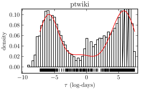
Figure 2: Test simulation for the estimation of the user lifespan scales $\tau_{0,1}$. Histograms: empirical data from the Portuguese Wikipedia. Black bottom vertical lines: simulated observations. Red line: nonparametric (i.e. kernel) density estimate of simulated data. Simulation was performed with mean of clustered data and $\tau_{t}=3\mathrm{h}$. Confidence $\varepsilon=0.24$. Other parameters estimated from data of the Portuguese Wikipedia.

4.5.2 Activity rates

Here we want to quantify the rates of activity for two processes: the arrival of new users and the creation of new pages. In our model these two processes are Poisson processes with a homogeneous rate of activity. Thus, our objective here is to quantify the average activity rate for both processes, so that we set the right scale of both processes for our calibration simulations. We estimate both rates from data.

To compute the rate of new users joining the community, we would need the daily rate of new account creation. Unfortunately, the time stamps for the creation of the accounts are not released to the public for obvious privacy reasons. As an approximation, we use the time stamp of the first edit. The daily volume of new users is then simply obtained by binning by date. Once we have the daily volumes, we just compute $\hat{\rho}_{u}=\overline{\rho}$. A similar method was used for estimating $\rho_{p}$ using the time stamp at which the page was created. This is simply the time stamp of the first contribution, which can be obtained from our raw data (see Section 2) by grouping by page id instead of by user id.

5 Results

For each Wikipedia in our dataset we sampled a maximin lhs design with 50 points, estimated the auxiliary parameters of the gmm, and estimated the parameters of the GP emulator. For the choice of the auxiliary model, we tested both mixtures of $k=2,3$ components, with and without data truncation. Before performing the final step in Eq. (5), we computed several diagnostic measures for each step of the calibration technique outlined in Figure 1.

5.1 Approximation of auxiliary parameters via Gaussian process

The choice of a good auxiliary model is important because $\boldsymbol{\beta}\left(\boldsymbol{\theta}\right)$ must be able to capture the features of the data well enough to be able to discriminate between different choices of the parameters of the agent-based model $\boldsymbol{\theta}$.

Identifiability may be hindered if multiple values of $\boldsymbol{\theta}$ result in similar values of $\boldsymbol{\beta}$. A quick way to check this is to plot $\boldsymbol{\beta}$, parametrized by $\boldsymbol{\theta}$, and see if the curve crosses over itself at one or more points, that is, if $\exists\boldsymbol{\theta}^{\prime},\boldsymbol{\theta}^{\prime\prime},\boldsymbol{\theta}^{\prime}\neq\boldsymbol{\theta}^{\prime\prime}$ s.t. $\boldsymbol{\beta}\left(\boldsymbol{\theta}^{\prime}\right)=\boldsymbol{\beta}\left(\boldsymbol{\theta}^{\prime\prime}\right)$.

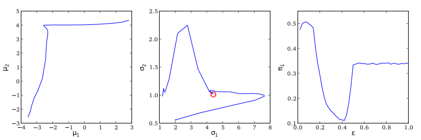
Figure 3: Auxiliary parameters as a function of $\varepsilon$. Auxiliary model: gmm with 2 components. Implicit and explicit parametric plots of parameter $\varepsilon$. Left: $\mu_{1}$ versus $\mu_{2}$; center: $\sigma_{1}$ versus $\sigma_{2}$; and right: $\pi_{1}$ versus $\varepsilon$.

For illustrative purpose, we assessed the identifiability of the gmm model on our model of peer production. Figure 3 reports the result of the test. We let $\varepsilon$ range in the interval $\left(0,1\right)$ and used the original (i.e. without edit cascades) peer production model to produce parametric plots of the parameters of the auxiliary model $\boldsymbol{\beta}\left(\varepsilon\right)$, as a function of $\varepsilon$. The auxiliary model used in Fig. 3 was a simple gmm with two components, for a total of five parameters: two means ($\mu_{1}$ and $\mu_{2}$), two variances ($\sigma_{1}$ and $\sigma_{2}$), and one weighting coefficient ($\pi_{1}$). We produced graphs only for the three most meaningful combinations of the ten possible pairwise choices of these parameters. The first two plots ($\mu_{1}$ vs. $\mu_{2}$ and $\sigma_{1}$ vs. $\sigma_{2}$) are parameterized implicitly by $\varepsilon$, while the last one reports the behavior of $\pi_{1}$ versus $\varepsilon$ explicitly. Close inspection of Figure 3 does not show any evident cross-overs. Cusps like the one present in the center plot (circled red), are less critical for identifiability, but may still cause computational problems if a local optimization technique to estimate the auxiliary parameters is used. Other cusps may be present in the plots for the other combinations, which we did not produce for this simpler model; our estimation technique for the auxiliary model, however, is based on Expectation Maximization and thus the presence of cusps should not present significant problems.

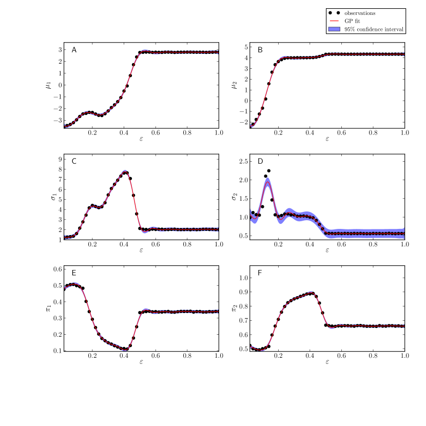
Figure 4: Gaussian Process approximation of auxiliary model. The abm model was simulated at 50 evenly spaced values of $\varepsilon\in\left[0,1\right]$, gmm parameters ($k=2$) were estimated and fit to a univariate gp. $x$-axis: bounded confidence $\varepsilon$, $y$-axis: gmm parameter. Red line: gp fit. Black dots: estimated parameter. Purple area: 95% confidence interval.

The next step is to assess the gp approximation. We fit one Gaussian process for each parameter of the gmm. In Figure 4 we show the result the gp approximation based on a learning set of 50 vectors of gmm parameters obtained from as many runs of the agent-based model. In the figure, the blue area represents the 95% confidence interval of the approximation, which shows a very tight approximation. Note that there is no change in the lifespan distribution for $\varepsilon\geq 0.5$, which is due to the bounded confidence dynamics: in $\left[0,1\right]$ the dynamics of agreement always result in a full consensus case when $\varepsilon\geq\nicefrac{\textrm{1}}{\textrm{2}}$, and thus the average lifespan of the population is $\tau_{0}$ regardless of the value of $\varepsilon$ [28].

5.2 Sensitivity analysis of auxiliary parameters

Table 4: Decomposition of variance, gmm, $k=3$. Portuguese Wikipedia. Top panel: main effects. Lower panel: total interaction effects.

Variable	Variance	$p_{\mathrm{rollback}}$	$\mu$	$\varepsilon$	$c_{s}$	$c_{p}$
$\mu_{1}$	1.503	0.023	0.038	0.389	0.095	0.020
$\mu_{2}$	16.618	0.036	0.012	0.709	0.022	0.018
$\mu_{3}$	11.331	0.031	0.028	0.698	0.055	0.027
$\sigma_{1}$	0.970	0.014	0.029	0.369	0.153	0.026
$\sigma_{2}$	1.288	0.016	0.044	0.309	0.125	0.068
$\sigma_{3}$	0.071	0.041	0.025	0.499	0.055	0.018
$\pi_{1}$	0.015	0.118	0.012	0.145	0.050	0.089
$\pi_{2}$	0.039	0.054	0.014	0.304	0.232	0.038
$\mu_{1}$	1.503	0.148	0.227	0.608	0.378	0.096
$\mu_{2}$	16.618	0.115	0.084	0.845	0.138	0.078
$\mu_{3}$	11.331	0.124	0.150	0.780	0.116	0.086
$\sigma_{1}$	0.970	0.151	0.186	0.585	0.399	0.109
$\sigma_{2}$	1.288	0.264	0.337	0.465	0.272	0.306
$\sigma_{3}$	0.071	0.168	0.157	0.733	0.241	0.122
$\pi_{1}$	0.015	0.290	0.259	0.506	0.288	0.382
$\pi_{2}$	0.039	0.202	0.228	0.492	0.363	0.236

Table 5: Decomposition of variance, truncated gmm, $k=2$. Italian Wikipedia. Top panel: main effects. Lower panel: total interaction effects.

Variable	Variance	$p_{\mathrm{rollback}}$	$\mu$	$\varepsilon$	$c_{s}$	$c_{p}$
$\mu_{1}$	1.312	0.075	0.073	0.270	0.133	0.060
$\mu_{2}$	2.845	0.037	0.032	0.771	0.043	0.014
$\sigma_{1}$	0.533	0.077	0.076	0.281	0.139	0.057
$\sigma_{2}$	0.018	0.019	0.088	0.138	0.097	0.073
$\pi_{1}$	0.042	-0.006	0.009	0.779	0.105	0.007
$\mu_{1}$	1.312	0.209	0.384	0.477	0.377	0.088
$\mu_{2}$	2.845	0.107	0.048	0.866	0.108	0.054
$\sigma_{1}$	0.533	0.214	0.355	0.479	0.375	0.085
$\sigma_{2}$	0.018	0.188	0.423	0.435	0.489	0.182
$\pi_{1}$	0.042	0.032	0.068	0.805	0.171	0.041

Table 6: Decomposition of variance, gmm. French Wikipedia. Top panel: main effects. Lower panel: total interaction effects.

Variable	Variance	$p_{\mathrm{rollback}}$	$\mu$	$\varepsilon$	$c_{s}$	$c_{p}$
$\mu_{1}$	0.511	0.012	0.037	0.294	0.127	-0.014
$\mu_{2}$	2.323	-0.001	-0.002	0.819	0.007	-0.014
$\sigma_{1}$	0.470	0.018	0.044	0.295	0.144	-0.008
$\sigma_{2}$	0.020	0.001	0.037	0.165	0.043	0.010
$\pi_{1}$	0.041	-0.009	-0.013	0.793	0.090	-0.002
$\mu_{1}$	0.511	0.152	0.317	0.534	0.449	0.081
$\mu_{2}$	2.323	0.065	0.034	0.925	0.102	0.049
$\sigma_{1}$	0.470	0.161	0.280	0.521	0.458	0.070
$\sigma_{2}$	0.020	0.187	0.328	0.570	0.573	0.114
$\pi_{1}$	0.041	0.030	0.057	0.846	0.166	0.034

For a more quantitative assessment of the gmm model as an auxiliary model, we saw how sensitive each auxiliary parameter was to changes in the inputs of the agent-based model. This is essentially a factor screening exercise. Moreover, sensitivity indices can also be used to define the matrix $\boldsymbol{W}$ of eq. (5). We performed a global sensitivity analysis of the auxiliary parameters. We computed main and total interaction effect indices using a decomposition of variance based on the winding stairs method [14, 61].

We performed the sensitivity analyses for each type of gmm and for each dataset. For convenience here we report only the results for the choice of the auxiliary model that we effectively used later in the calibration (tables 4–6), but found nonetheless similar results for the other combinations. Small negative indices near zero were due to the sampling uncertainty in the winding stairs method.

The result of the sensitivity analysis shows that the auxiliary parameters with the highest variance were the locations $\mu$ of the mixture components (i.e. the means) and, to some extent, the variances $\sigma$. A truncated model seemed to decrease the difference in variability between the mixture means. Most importantly, main effect indices show that the confidence parameter ($\varepsilon$) was responsible for most of the variability of the auxiliary parameters. In summary, the auxiliary model was especially sensitive to changes in $\varepsilon$, weakly sensitive to changes in $c_{s}$, and almost insensitive to other parameters.

5.3 Cross-validation

Table 7: Results of leave-one-out cross-validation. Coefficient of determination $R^{2}$. For each language, the best $R^{2}$ attained over parameter $\varepsilon$ is shown in bold.

	$\mu$	$\varepsilon$	$p_{\mathrm{rollback}}$	$c_{s}$	$c_{p}$
Portuguese
gmm, $k=2$	0.02	0.73	0.00	0.13	0.02
gmm, $k=3$	0.03	0.86	0.16	0.02	0.01
tgmm, $k=2$	0.01	0.70	0.01	0.36	0.01
tgmm, $k=3$	0.04	0.85	0.00	0.28	0.01
Italian
gmm, $k=2$	0.00	0.91	0.01	0.66	0.09
gmm, $k=3$	0.02	0.90	0.01	0.30	0.03
tgmm, $k=2$	0.02	0.93	0.03	0.75	0.01
tgmm, $k=3$	0.00	0.85	0.00	0.42	0.03
French
gmm, $k=2$	0.00	0.91	0.01	0.61	0.04
gmm, $k=3$	0.01	0.90	0.03	0.33	0.01
tgmm, $k=2$	0.01	0.76	0.00	0.69	0.08
tgmm, $k=3$	0.08	0.86	0.16	0.35	0.09

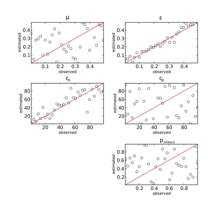
Figure 5: Leave-one-out cross validation. $x$-axis: observed holdout parameter values obtained by lhs. $y$-axis: indirect inference estimates based on remaining data. Simulations were carried out with the parameterization for the Italian Wikipedia (see Table 3); the auxiliary model was a truncated gmm, $k=2$. The red line has slope equal to 1 and serves a guide to the eye.

Finally, we used leave-one-out cross-validation to quantify the accuracy of indirect inference in reconstructing the parameters of the model. Using lhs we sampled $N$ vectors of parameters and simulated from the agent-based model to obtain as many samples of user activity lifespans. We then set aside one pair $\left(\boldsymbol{\theta}_{h},\boldsymbol{\tau}_{h}\right)$ as test set (the holdout) and used the remaining $N-1$ pairs as a learning set for the indirect inference technique, which we used to estimate $\boldsymbol{\hat{\theta}_{h}}$ from the synthetic lifespan data $\boldsymbol{\tau}_{h}$. Repeating this exercise for $h=1\ldots N$, we can the plot the estimated abm parameters as a function of the true ones, and compute coefficient of determination $R^{2}$ to assess the performance of the calibration.

We performed several cross-validations, for each language and auxiliary model combination. For each of those, we tested both a weighted and an unweighted indirect inference technique. In the weighted case, the diagonal of the matrix $\boldsymbol{W}$ from Eq. (5) was set to the variances of the parameters from the global sensitivity analysis (see Tables 4–6), while in the unweighted case $\boldsymbol{W}=\boldsymbol{I}$. Surprisingly, the best results were those with no weighting, which are those we choose to report here. Table 7 reports the results.

While accuracy, as determined by the $R^{2}$, varied sometimes appreciably across flavors of the auxiliary model and languages, it seemed consistent with the results of the global sensitivity analysis. The best-performing auxiliary model for each language was selected looking at the $R^{2}$ for the confidence parameter (in bold in the table). As a graphical companion to the table, Figure 5 shows the cross-validation plot for the Italian case. As expected, the accuracy is excellent for the confidence parameter $\varepsilon$ and good for the initial motivation $c_{s}$, while for other parameters no clear linear trend can be discerned.

5.4 Indirect inference

Table 8: Calibrated parameters with standard errors.

wiki	$p_{\mathrm{rollback}}$	$\mu$	$\varepsilon$	$c_{s}$	$c_{p}$
pt	0.52 ±0.01	0.46 ±0.00	0.39 ±0.00	70.78 ±0.80	51.56 ±0.79
it	0.36 ±0.00	0.21 ±0.00	0.49 ±0.00	53.81 ±0.61	58.31 ±0.57
fr	0.02 ±0.01	0.02 ±0.00	0.49 ±0.00	3.79 ±0.86	89.37 ±0.77

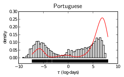
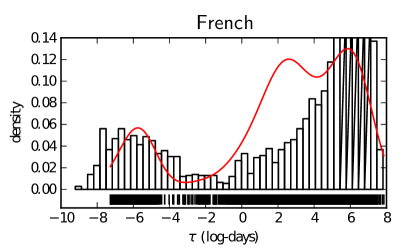
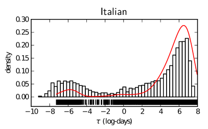
Figure 6: Comparison between empirical data (histograms) and simulated data (kernel density estimate, red line), obtained from the calibrated model.

Having tested the accuracy of the indirect inference technique and selected the best auxiliary models for each language, we finally applied it to the empirical data to get estimates of the parameters of our model. Table 8 reports the results of the calibration; standard errors were computed on a bootstrapped sample with 1000 observations.

With these, we simulated from the calibrated model. As a way to check the model fit visually, we plotted in Figure 6 a kernel density estimate of the synthetic data together with histograms of empirical data.

6 Discussion

Indirect inference is a promising framework for calibrating computational models, but its application requires some care and is not as straightforward as classic inference techniques such as maximum likelihood. In particular, it is important to assess independently the performance of the auxiliary model in capturing the salient aspects of the model. This is especially useful for assessing the accuracy of the model in estimating the various model parameters.

Useful diagnostic tests include parametric plots for assessing potential problems with identification (Fig. 3) and diagnostic plots of the gp emulator (Fig. 4). Moreover, the results of the cross-validation (Section 5.3) were consistent with those of the global sensitivity analysis of the auxiliary model (Section 5.2), which shows exactly how multiple independent methods can provide a comprehensive diagnostic picture of a calibration method before one sets out to apply it to a model.

Using the global sensitivity analysis and cross-validation we learned that the gmm model could capture well two parameters out of the five we tried to calibrate, namely the confidence bound $\varepsilon$ and the initial motivation $c_{s}$ (see Fig 5). While the result for $\varepsilon$ is expected, that for $c_{s}$ comes a bit as an interesting surprise, and can be explained by noting that this parameter is able to influence the location of the short-term component of lifespan distribution, a feature that the mixture model is indeed able to detect, albeit partially.

The method is not reliable at reconstructing the other three parameters, namely the speed $\mu$, the rollback probability $p_{\mathrm{rollback}}$, and the popularity dampening factor $c_{p}$, as evidenced by the coefficient of determination of the leave-one-out cross-validation. This means that we gained little by calibrating these parameters, and could have set them to the mid-range of their intervals before running the calibration simulations, thus calibrating a simpler model. The low sensitivity of the auxiliary model to these parameters may be due to the inability of the auxiliary model in capturing the patterns in the data, or to the norm formation model itself; that is, the model may be underdetermined by the data.

Because the Gaussian mixture model is generally regarded as a versatile model for complicate data, such as the user activity lifespan [17], we deem the latter a more likely explanation than the former.

Taken together, these results highlight how the choice of a good auxiliary model is critical to the successful application of indirect inference, and how factor screening via global sensitivity analysis can be leveraged to assess the quality of an auxiliary model. Conversely, one could also argue that the calibration exercise, as outlined here, is useful for assessing whether, and especially where, a model is underdetermined by the data, and thus it could point to an effective methodology for identifying the parts that may be simplified. Thus indirect inference could become a valuable tool in the toolbox of every agent-based modeling practitioner.

If, however, one would be interested in estimating their value, then the question remains open as to which approach should be used for calibrating reliably the remaining three parameters mentioned above. A different auxiliary model could be used, but the possibility of incorporating data variables other than the activity lifespan should be taken into account, since it would alleviate the under-determination problem. This is most pressing for a parameter like $p_{\mathrm{rollback}}$, which is supposed to play an important role in the mechanism of norm emergence, while it seems less critical for parameters like $\mu$ and $c_{p}$; in the first case, this parameter is considered less important for the dynamics of the bc model [12], while in the other the corresponding mechanism (page selection) may be just too complicated and thus could be dropped in favor of a simpler model.

Comparison of the prediction of the calibrated model with the empirical data (Fig. 6) shows discrepancies at a range of very short time scales ($\approx 10^{-8}\;\log\left(\dday\right)$), and a degree of overestimation of $\varepsilon$, resulting in a distribution that gives too much probability at large lifespan scales. Moreover, the estimates for the confidence bound $\varepsilon$ parameter (Tab. 8) are very close to the full consensus value $\varepsilon=0.5$; this is the value past which consensus is always the case, suggesting an over-estimation of this parameter. This would be in fact counter-intuitive, considered the general opinion that Wikipedia is a conflict-laden arena, and one straightforward implication would also be the absence of minority groups in the community of Wikipedia users, which seems also in contrast with general observation. Table 8 also shows large differences among the estimates for $c_{s}$. The calibration accuracy for this parameter is lower than for $\varepsilon$, which might explain these big differences.

For such a simplistic model, the results are nonetheless encouraging. Better fits could be attained with more sophisticate estimation of parameters such as the time scales $\tau_{0}$ and $\tau_{1}$, as well as by introducing a more sophisticated model of the distribution of the time between consecutive edits of users [57, 72]. The new parameters, if any, introduced by such models could be estimated separately, or possibly included in the indirect inference.

Evaluation of the model inadequacy, of the uncertainty in the predictions due to use of a surrogate model and parameter estimation and goodness of fit measures are of course all desirable improvements on the methods presented here [43, 40]. Statistical tests for goodness of fit exist for the classic indirect inference technique [32]; thus it would be interesting to see how to apply them when an additional layer of emulation is required, as it is in our case with the Gaussian Process.

7 Conclusions

We have presented a method for calibrating an agent-based model of the activity lifespan of users in a community of peer production. The method is especially suited for models with high-dimensional outputs and long simulation times, as is often the case in social simulation.

Peer production communities provide a unique opportunity to study the emergence of social norms. Norms, including social production norms, contribute to the distinctive culture of an online community and thus the process of community formation can be regarded more broadly as a process of cultural dynamics. Several agent-based models have been proposed to explain various aspects of the process of cultural formation in a generic setting [3, 56, 44, 13, 27]. It would be interesting to know whether these models could be empirically validated in some way, and calibration techniques such as the one presented here could prove useful to this end.

References

- [1] J. McKenzie Alexander. The Structural Evolution of Morality. Cambridge University Press, 2007.
- [2] Robert Axelrod. An evolutionary approach to norms. American Political Science Review, 80:1095–1111, 1986.
- [3] Robert Axelrod. The complexity of cooperation. Princeton Studies in Complexity. Princeton University Press, 1997.
- [4] Albert-László Barabási and Réka Albert. Emergence of scaling in random networks. Science, 286(5439):509–512, 1999.
- [5] Albert-Lázló Barabási. The origin of bursts and heavy tails in human dynamics. Nature, 435(7039):207–211, 2005.
- [6] Maria J Bayarri, James O Berger, Rui Paulo, Jerry Sacks, John A Cafeo, James Cavendish, Chin-Hsu Lin, and Jian Tu. A framework for validation of computer models. Technometrics, 49(2):138–154, 2007.
- [7] Y. Benkler. The wealth of networks: How social production transforms markets and freedom. Yale University Press, 2006.
- [8] Carlo Bianchi, Pasquale Cirillo, Mauro Gallegati, and Pietro Vagliasindi. Validating and calibrating agent-based models: A case study. Computational Economics, 30(3):245–264, 10 2007.
- [9] C. Bicchieri. The grammar of society: The nature and dynamics of social norms. Cambridge University Press, 2005.
- [10] Eric Bonabeau. Agent-based modeling: Methods and techniques for simulating human systems. Proceedings of the National Academy of Sciences of the United States of America, 99(Suppl 3):7280–7287, 2002.
- [11] Colin F. Camerer and Ernst Fehr. Measuring Social Norms and Preferences Using Experimental Games: A Guide for Social Scientists, chapter 3, pages 55–95. Oxford University Press, 2004.
- [12] Claudio Castellano, Santo Fortunato, and Vittorio Loreto. Statistical physics of social dynamics. Rev. Mod. Phys., 81(2):591–646, May 2009.
- [13] Damon Centola, Juan Carlos González-Avella, Víctor M. Eguíluz, and Maxi San Miguel. Homophily, cultural drift, and the co-evolution of cultural groups. Journal of Conflict Resolution, 51(6):905–929, 2007.
- [14] Karen Chan, Andrea Saltelli, and Stefano Tarantola. Winding stairs: A sampling tool to compute sensitivity indices. Statistics and Computing, 10:187–196, 2000.
- [15] Coye Cheshire and Judd Antin. The social psychological effects of feedback on the production of internet information pools. Journal of Computer-Mediated Communication, 13(3):705–727, 2008.
- [16] Giovanni Luca Ciampaglia. A bounded confidence approach to understand user participation in peer production systems. In Third International Conference on Social Informatics (SocInfo’11), LNCS, Singapore, 6 - 8 October 2011. Springer Verlang.
- [17] Giovanni Luca Ciampaglia and Alberto Vancheri. Empirical analysis of user participation in online communities: the case of Wikipedia. In Proceedings of ICWSM, 2010.
- [18] Andrea Ciffolilli. Phantom authority, self-selective recruitment and retention of members in virtual communities: The case of wikipedia. First Monday, 8(12), Dec 2003.
- [19] William A. V. Clark and Mark Fossett. Understanding the social context of the Schelling segregation model. Proceedings of the National Academy of Sciences, 105(11):4109–4114, 2008.
- [20] Garrett M. Dancik, Douglas E. Jones, and Karin S. Dorman. Parameter estimation and sensitivity analysis in an agent-based model of Leishmania major infection. Journal of Theoretical Biology, 262(3):398 – 412, 2010.
- [21] E.L. Deci, R. Koestner, and R.M. Ryan. A meta-analytic review of experiments examining the effects of extrinsic rewards on intrinsic motivation. Psychological bulletin, 125(6):627, 1999.
- [22] G Deffuant, F Amblard, G Weisbuch, and T Faure. How can extremism prevail? a study based on the relative agreement interaction model. J. Art. Soc. Soc. Sim., 5(4):paper 1, 2002.
- [23] Guillame Deffuant, David Neau, Frederic Amblard, and Gérard Weisbuch. Mixing beliefs among interacting agents. Adv. Comp. Sys., 3:87–98, 2001.
- [24] Stephen P. Ellner and John Guckenheimer. Dynamic Models in Biology. Princeton University Press, 2006.
- [25] Joshua M Epstein and Robert Axtell. Growing artifical societies: social sciences from the bottom up. The MIT Press, Cambridge, MA, USA, 1996.
- [26] Daniel C. Feldman. The development and enforcement of group norms. The Academy of Management Review, 9(1):pp. 47–53, 1984.
- [27] Andreas Flache and Michael W. Macy. Local convergence and global diversity: From interpersonal to social influence. Journal of Conflict Resolution, 55(6):970–995, 2011.
- [28] S. Fortunato. Universality of the threshold for complete consensus for the opinion dynamics of Deffuant et al. International Journal of Modern Physics C, 15:1301–1307, 2004.
- [29] Santo Fortunato and Claudio Castellano. Scaling and universality in proportional elections. Phys. Rev. Lett., 99(13):138701, Sep 2007.
- [30] Daniel Gillespie. Exact stochastic simulation of coupled chemical reactions. Journal of Physical Chemistry, 81(25):2340–2361, 1977.
- [31] M. Gilli and P. Winker. A global optimization heuristic for estimating agent based models. Computational Statistics & Data Analysis, 42(3):299–312, March 2003.
- [32] C Gouriéroux, A Monfort, and E Renault. Indirect inference. Journal Of Applied Econometrics, 8(Suppl. S):85–118, Dec 1993. Conference On Econometric Inference Using Simulation Techniques, Rotterdam, Netherlands, Jun 05-06, 1992.
- [33] Charles R. Graham. A model of norm development for computer-mediated teamwork. Small Group Research, 34(3):322–352, 2003.
- [34] Lei Guo, Enhua Tan, Songqing Chen, Xiaodong Zhang, and Yihong (Eric) Zhao. Analyzing patterns of user content generation in online social networks. In KDD ’09: Proceedings of the 15th ACM SIGKDD international conference on Knowledge discovery and data mining, pages 369–378, New York, NY, USA, 2009. ACM.
- [35] Aaron Halfaker, Aniket Kittur, and John Riedl. Don’t bite the newbies: how reverts affect the quantity and quality of wikipedia work. In Proceedings of the 7th International Symposium on Wikis and Open Collaboration, WikiSym ’11, pages 163–172, New York, NY, USA, 2011. ACM.
- [36] W.D. Hamilton. The genetical evolution of social behaviour. i. Journal of Theoretical Biology, 7(1):1–16, 1964.
- [37] Russell Hardin. Collective action. Resources for the Future. Johns Hopkins University Press, 1982.
- [38] Rainer Hegselmann and Ulrich Krause. Opinion dynamics and bounded confidence–models, analysis, and simulation. J. Art. Soc. Soc. Sim., 5(3):paper 2, 2002.
- [39] Katrin Heitmann, David Higdon, Charles Nakhleh, and Salman Habib. Cosmic calibration. The Astrophysical Journal Letters, 646(1):L1, 2006.
- [40] Dave Higdon, Marc Kennedy, James C. Cavendish, John A. Cafeo, and Robert D. Ryne. Combining field data and computer simulations for calibration and prediction. SIAM J. Sci. Comput., 26(2):448–466, February 2005.
- [41] A.O. Hirschman. Exit, voice, and loyalty: Responses to decline in firms, organizations, and states, volume 25. Cambridge, Mass.: Harvard University Press, 1970.
- [42] BE Kendall, SP Ellner, E McCauley, SN Wood, CJ Briggs, WM Murdoch, and P Turchin. Population cycles in the pine looper moth: Dynamical tests of mechanistic hypotheses. Ecological Monographs, 75(2):259–276, May 2005.
- [43] Marc C. Kennedy and Anthony O’Hagan. Bayesian calibration of computer models. Journal of the Royal Statistical Society: Series B (Statistical Methodology), 63(3):425–464, 2001.
- [44] Konstantin Klemm, Víctor M. Eguíluz, Raúl Toral, and Maxi San Miguel. Global culture: A noise-induced transition in finite systems. Phys. Rev. E, 67:045101, Apr 2003.
- [45] David Lazer, Alex Pentland, Lada Adamic, Sinan Aral, Albert-László Barabási, Devon Brewer, Nicholas Christakis, Noshir Contractor, James Fowler, Myron Gutmann, Tony Jebara, Gary King, Michael Macy, Deb Roy, and Marshall Van Alstyne. Computational social science. Science, 323(5915):721–723, 2009.
- [46] Josh Lerner and Jean Tirole. Some simple economics of open source. The Journal of Industrial Economics, 50(2):197–234, 2002.
- [47] R Dean Malmgren, Daniel B Stouffer, Adilson E Motterb, and Luís A N Amaral. A poissonian explanation for heavy tails in e-mail communication. Proc. Natl. Acad. Sci. U. S. A., 105(47):18153–18158, Nov 2008.
- [48] Michael Mäs, Andreas Flache, and Dirk Helbing. Individualization as driving force of clustering phenomena in humans. PLoS Computational Biology, 6(10):e1000959, October 2010.
- [49] Daniel McFadden. A method of simulated moments for estimation of discrete response models without numerical integration. Econometrica, 57(5):995–1026, September 1989.
- [50] Miller McPherson, Lynn Smith-Lovin, and James M Cook. Birds of a feather: Homophily in social networks. Annual Review of Sociology, 27(1):415–444, 2001.
- [51] Max D. Morris and Toby J. Mitchell. Exploratory designs for computational experiments. Journal of Statistical Planning and Inference, 43(3):381–402, 1995.
- [52] S. Moscovici, E. Lage, and M. Naffrechoux. Influence of a consistent minority on the responses of a majority in a color perception task. Sociometry, 32(4):pp. 365–380, 1969.
- [53] J.G. Neff, D. Laniado, K. Kappler, Y. Volkovich, P. Aragón, and A. Kaltenbrunner. Jointly they edit: examining the impact of community identification on political interaction in wikipedia. arXiv preprint arXiv:1210.6883, 2012.
- [54] Karl-Dieter Opp. How do norms emerge? an outline of a theory. Mind & Society, 2:101–128, 2001. 10.1007/BF02512077.
- [55] Elinor Ostrom. Collective action and the evolution of social norms. The Journal of Economic Perspectives, 14(3):pp. 137–158, 2000.
- [56] Domenico Parisi, Federico Cecconi, and Francesco Natale. Cultural change in spatial environments. Journal of Conflict Resolution, 47(2):163–179, 2003.
- [57] Filippo Radicchi. Human activity in the web. Phys. Rev. E: Stat., Nonlinear, Soft Matter Phys., 80(2):026118, Aug 2009.
- [58] Sheizaf Rafaeli and Yaron Ariel. Psychological aspects of cyberspace: Theory, research, applications, chapter Online Motivational Factors: Incentives for Participation and Contribution in Wikipedia, pages 243–267. Cambridge University Press, 2008.
- [59] Joseph M. Jr. Reagle. Good Faith Collaboration–The Culture of Wikipedia. The MIT Press, 2007.
- [60] Y. Ren, R. Kraut, S. Kiesler, and P. Resnick. Evidence-based social design: Mining the social sciences to build online communities, chapter Encouraging commitment in online communities, pages 77–124. MIT Press, Cambridge, MA, 2012.
- [61] Andrea Saltelli, Stefano Tarantola, Francesca Campolongo, and Marco Ratto. Sensitivity Analysis in Practice–A guide to Assessing Scientific Models. John Wiley & Sons, Ltd., 2004.
- [62] T.J. Santner, B. Williams, and W. Notz. The Design and Analysis of Computer Experiments. Springer-Verlag, NY, 2003.
- [63] Thomas C. Schelling. Dynamic models of segregation. The Journal of Mathematical Sociology, 1(2):143–186, 1971.
- [64] A. A. Smith. Estimating nonlinear time-series models using simulated vector autoregressions. Journal of Applied Econometrics, 8(S1):S63–S84, 1993.
- [65] Anthony A. Jr. Smith. indirect inference. In Steven N. Durlauf and Lawrence E. Blume, editors, The New Palgrave Dictionary of Economics. Palgrave Macmillan, Basingstoke, 2008.
- [66] Pawel Sobkowicz. Modelling opinion formation with physics tools: Call for closer link with reality. Journal Artificial Societies and Social Simulation, 12(1):11, 2009.
- [67] H Tajfel. Social psychology of intergroup relations. Annual Review of Psychology, 33(1):1–39, 1982.
- [68] J. C. Turner. Rediscovering the social group: A self-categorization theory. Blackwell Publishers, London, 1989.
- [69] Dennis M Wilkinson. Strong regularities in online peer production. In Proceedings of the 9th ACM conference on Electronic commerce, Chicago, Illinois USA, 2008.
- [70] Paul Windrum, Giorgio Fagiolo, and Alessio Moneta. Empirical validation of agent-based models: Alternatives and prospects. Journal of Artificial Societies and Social Simulation, 10(2):8, 2007.
- [71] Simon N. Wood. Statistical inference for noisy nonlinear ecological dynamic systems. Nature, 466(7310):1102–U113, August 26 2010.
- [72] Ye Wu, Changsong Zhou, Jinghua Xiao, Jürgen Kurths, and Hans Joachim Schellnhuber. Evidence for a bimodal distribution in human communication. Proceedings of the National Academy of Sciences, 107(44):18803–18808, 2010.
- [73] D. Zhang, K. Prior, and M. Levene. How long do wikipedia editors keep active? In Proceedings of the 8th International Symposium on Wikis and Open Collaboration (Wikisym ‘12), 2012.