Time persistency of floating particle clusters in free-surface turbulence

Abstract

Abstract We study the dispersion of light particles floating on a flat shear-free surface of an open channel in which the flow is turbulent. This configuration mimics the motion of buoyant matter (e.g. phytoplankton, pollutants or nutrients) in water bodies when surface waves and ripples are smooth or absent. We perform direct numerical simulation of turbulence coupled with Lagrangian particle tracking, considering different values of the shear Reynolds number ($Re_{\tau}=171$ and $509$) and of the Stokes number ($0.06<St<1$ in viscous units). Results show that particle buoyancy induces clusters that evolve towards a long-term fractal distribution in a time much longer than the Lagrangian integral fluid time scale, indicating that such clusters over-live the surface turbulent structures which produced them. We quantify cluster dynamics, crucial when modeling dispersion in free-surface flow turbulence, via the time evolution of the cluster correlation dimension.

I Introduction

Buoyant particles transported by three-dimensional incompressible turbulence are known to distribute non-uniformly within the flow [1,2,3,4]. In the particular case of light tracer particles (referred to as floaters hereinafter) in free-surface turbulence, non-uniform distribution is observed on the surface, where floaters form clusters by accumulating along patchy and string-like structures [3]. Clustering occurs even if floaters have no inertia, and in the absence of floater-floater interaction, surface tension effects, or wave motions [3]. Differently from the case of inertial particles, in which clustering is driven by inertia and arises when particle trajectories deviate from flow streamlines [5], clusters are controlled by buoyancy, which forces floaters on the surface. The physical mechanism governing buoyancy-induced clustering is closely connected to the peculiar features of free-surface turbulence, which is characterized by sources (resp. sinks) of fluid velocity where the fluid is moving upward (resp. downward) [1]. Once at the surface, floaters follow fluid motions passively and leave quickly the upwelling regions gathering in downwelling regions: here, fluid can escape from the surface and sink whereas floaters can not, precisely because of buoyancy [3].

In a series of recent papers [2,3,4] it was shown that floater clusters in free-surface turbulence form a compressible system that evolves towards a fractal distribution in several large-eddy turnover times (measured at the free-surface) and at an exponential rate. The macroscopic manifestation of this behavior is strong depletion of floaters in large areas of the surface and very high particle concentration along narrow string-like regions, which are typical of scum coagulation on the surface of the sea [4]. From a statistical viewpoint, this is reflected by a peaked probability distribution function of particle concentration with power-law tails. A proper description of such power-law distribution requires a clear understanding of the mechanism by which floaters are segregated into filamentary clusters. In this letter we examine such mechanism from a phenomenological point of view, and we also quantify cluster dynamics in connection with the characteristic timescale of the surface vortices. This analysis is of fundamental interest since it quantifies the temporal persistency of clusters with respect to the dominant surface flow scales, but reflects practically towards modeling of dispersion in many surface transport phenomena, such as the spreading of phytoplankton, pollutants and nutrients in oceanic flow [4].

II Problem Formulation and Numerical Methodology

The flow field is calculated by integrating incompressible continuity and Navier-Stokes equations. In dimensionless form:

$$\frac{\partial u_{i}}{\partial x_{i}}=0\leavevmode\nobreak\ ,\leavevmode\nobreak\ \leavevmode\nobreak\ \leavevmode\nobreak\ \frac{\partial u_{i}}{\partial t}=-u_{j}\frac{\partial u_{i}}{\partial x_{j}}+\frac{1}{Re_{\tau}}\frac{\partial^{2}u_{i}}{\partial x_{j}\partial x_{j}}-\frac{\partial p}{\partial x_{i}}+\delta_{1,i}\leavevmode\nobreak\ ,$$ (1)

with $u_{i}$ the $i^{th}$ component of the fluid velocity, $p$ the fluctuating kinematic pressure, $\delta_{1,i}$ the mean pressure gradient driving the flow, and $Re_{\tau}=hu_{\tau}/\nu$ the shear Reynolds number based on the channel depth $h$ and the shear velocity $u_{\tau}=\sqrt{h|\ \delta_{1,i}|\ /\rho}$. Eqns. (1) are solved directly using a pseudo-spectral method that transforms field variables into wavenumber space, through Fourier representations for the streamwise and spanwise directions (using $k_{x}$ and $k_{y}$ wavenumbers respectively) and a Chebyshev representation for the wall-normal non-homogeneous direction (using $T_{n}$ coefficients). A two-level explicit Adams-Bashfort scheme for the non-linear terms and an implicit Crank-Nicolson method for the viscous terms are employed for time advancement 6.

Floaters motion is described by a set of ordinary differential equations for velocity ${\mathbf{v}}_{p}$ and position ${\mathbf{x}}_{p}$ at each time step. In vector form:

$$\frac{\mbox{d}{\mathbf{x}}_{p}}{\mbox{d}t}={\mathbf{v}}_{p}\leavevmode\nobreak\ ,\leavevmode\nobreak\ \leavevmode\nobreak\ \frac{\mbox{d}{\mathbf{v}}_{p}}{\mbox{d}t}=\frac{(\rho_{p}-\rho_{f})}{\rho_{p}}{\mathbf{g}}+\frac{({\mathbf{u}}_{@p}-{\mathbf{v}}_{p})}{\tau_{p}}f(Re_{p})$$ (2)

where ${\mathbf{u}}_{@p}$ is the fluid velocity at the floater position, interpolated with 6th-order Lagrange polynomials, $\rho_{p}$ (resp. $\rho_{f}$) is the floater (resp. fluid) density, and $\tau_{p}=\frac{\rho_{p}\,d_{p}^{2}}{18\,\rho_{f}\nu}$ is the floater relaxation time based on the diameter $d_{p}$. The Stokes drag coefficient is computed using the Schiller-Naumann non-linear correction ($f(Re_{p})=(1+0.15\,Re_{p}^{0.687})$) required for floater Reynolds number $Re_{p}=|{\mathbf{u}}_{@p}-{\mathbf{v}}_{p}|\,d_{p}/\nu>1$. To calculate individual trajectories, a Lagrangian tracking routine is coupled to the flow solver [5]. Periodic boundary conditions are imposed on floaters moving outside the computational domain in the homogeneous directions.Eqns. (2) are advanced in time using a 4th-order Runge-Kutta scheme starting from a random distribution of floaters with velocity ${\mathbf{v}}_{p}(t=0)\equiv{\mathbf{u}}_{@p}(t=0)$.

Results presented in this paper are relative to two values of the shear Reynolds number: $Re_{\tau}^{L}=171$ and $Re_{\tau}^{H}=509$ corresponding, respectively, to shear velocity $u_{\tau}^{L}=0.00605\ ms^{-1}$ and $u_{\tau}^{H}=0.018\ ms^{-1}$. The size of the computational domain in wall units is $L_{x}^{+}\times L_{y}^{+}\times L_{z}^{+}=2\pi Re_{\tau}\times\pi Re_{\tau}\times Re_{\tau}$, discretized with $128\times 128\times 129$ grid points ($k_{x}=i2\pi/L_{x}$, $k_{y}=j2\pi/L_{y}$ with $i,j=1,...,128$, and $T_{n}(z)=\cos[n\cdot\cos^{-1}(z/h)]$ with $n=1,...,129$ before de-aliasing) at $Re_{\tau}^{L}$ and with $256\times 256\times 257$ grid points ($i,j=256$ and $n=257$ before de-aliasing) at $Re_{\tau}^{H}$. Samples of ${\cal{N}}=2\cdot 10^{5}$ floaters characterized by specific density $S=\rho_{p}/\rho_{f}=0.5$ and diameter $d_{p}=250\leavevmode\nobreak\ \mu m$ (a value in the size range of large phytoplankton cells [7]) were considered. The corresponding values of the non-dimensional response time (Stokes number) $St=\tau_{p}/\tau_{f}$ with $\tau_{f}=\nu/u_{\tau}^{2}$ the viscous timescale of the flow, are $St^{L}=0.064$ at $Re_{\tau}^{L}$ and $St^{H}=0.562$ at $Re_{\tau}^{H}$. Floaters with density much less than that of the fluid were considered on purpose to confine their motion to the free surface and produce a behavior which resembles not at all that of neutrally buoyant, non-inertial particles.

III Results and discussion

III.1 Characterization of free-surface turbulence through energy spectra

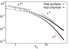
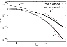
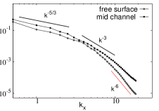
Figure 1: One-dimensional (streamwise) energy spectra of the streamwise ($E_{x}(k_{x})$, panels (a) and (c)) and spanwise ($E_{y}(k_{x})$, panels (b) and (d)) surface-parallel velocity fluctuations. Spectra are computed at the free surface ($z^{+}=0$, circles) and at the channel center ($z^{+}=254.6$ at $Re_{\tau}^{H}$, $z^{+}=85.5$ at $Re_{\tau}^{L}$, squares).

Turbulent flow structures near the free surface of an open channel have been investigated in several previous studies [12,6,10,9,8,11,13]. All these studies show that surface structures are generated and sustained by bursting phenomena that are continuously produced by wall shear turbulence inside the buffer layer. Specifically, bursts emanate from the bottom of the channel and produce upwelling motions of fluid as they are convected toward the free surface. Near the surface, turbulence is restructured and nearly two-dimensionalized due to damping of vertical fluctuations [14]: upwellings appear as two-dimensional sources for the surface-parallel fluid velocity and alternate to sinks associated with downdrafts of fluid from the surface to the bulk. Through sources fluid elements at the surface are replaced with fluid from the bulk, giving rise to the well-known surface-renewal events [10]. Whirlpool-like vortices may also form in the high-shear region between the edges of two closely-adjacent upwellings. This phenomenology has been long recognized to produce flow with properties that differ from those typical of two-dimensional incompressible Navier-Stokes turbulence [15,1]. These properties can be quantified examining the energy spectra of the fluid velocity fluctuations on the surface [11], shown in Fig. 1 for the case of statistically-steady turbulence. To emphasize direction-related aspects of the energy spectra, results for the surface-parallel velocities are examined in isolation: Panels (a) and (c) in Fig. 1 show the one-dimensional streamwise spectra of the streamwise velocity $E_{x}(k_{x})$ computed at the free surface (circles) and at the channel center (squares) in the $Re_{\tau}^{L}$ and $Re_{\tau}^{H}$ simulations, respectively; panels (b) and (d) show the spectra of the spanwise velocity $E_{y}(k_{x})$ in the same two regions. Solid lines represent the slope of the spectrum within the inertial regimes predicted by the Kraichnan-Leith-Batchelor phenomenology of two-dimensional turbulence [16,17]: $k_{x}^{-5/3}$, representing inverse cascade of energy to large flow scales, and $k_{x}^{-3}$, representing direct cascade of enstrophy to small flow scales. A collective analysis of spectra shown in Fig. 1 reveals that $-5/3$ range can be observed only for few of the lowest wavenumbers. A relatively larger range of high wavenumbers can be identified over which spectra exhibit a $-3$ scaling. In essence, there is a sort of reverse cascade with energy in the high wave numbers decaying rapidly, but low wave numbers (large vortices) decaying much more slowly. Examining $E_{x}(k_{x})$, we notice that the spectrum at the free surface is always below that computed in the center of the channel. Also, energy in the high-wavenumber portion of the spectrum decays more rapidly [11], roughly as $k^{-6}$: this tendency is particularly evident at $Re_{\tau}^{H}$ and indicates that only large-scale surface structures survive to the detriment of small-scale ones. Examining $E_{y}(k_{x})$, we observe that redistribution of energy from small to large scales in proximity of the free surface determines a cross-over between spectra at low wavenumbers (for both Reynolds numbers): this finding confirms further that small scale structures play little role in determining turbulence properties in this region of the flow.

III.2 Characterization of particle clustering through surface divergence

Most of the analyses for geophysical flows were conducted considering two-dimensional incompressible homogeneous isotropic turbulence [18,19]. In such flows the divergence of the velocity field is zero by construction. However, the divergence in real surface flows is defined as:

$$\nabla_{2D}=\frac{\partial u}{\partial x}+\frac{\partial v}{\partial y}=-\frac{\partial w}{\partial z}\leavevmode\nobreak\ ,$$ (3)

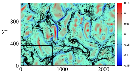
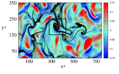
Figure 2: Correlation between floater clusters and surface divergence $\nabla_{2D}$: floaters segregate in $\nabla_{2D}<0$ regions (in blue, footprint of sub-surface downwellings) avoiding $\nabla_{2D}>0$ regions (in red, footprint of sub-surface upwellings). Panels: (a) $Re_{\tau}^{H}$, $t^{+}=180$ upon floater injection; (b) $Re_{\tau}^{L}$, $t^{+}=121$. The rectangle in panel (a) renders the relative domain size in the $Re_{\tau}^{L}$ simulation; the rectangle in panel (b) highlights the floater cluster shown in Fig. 4.

and does not vanish. Therefore floaters, forced to stay on surface, probe a compressible two-dimensional system [2], where velocity sources are regions of local flow expansion ($\nabla_{2D}>0$) generated by sub-surface upwellings and velocity sinks are regions of local compression ($\nabla_{2D}<0$) due to downwellings [1]. In Fig. 2 we provide a qualitative characterization of floater clustering on the free surface by correlating the instantaneous particle patterns with the colormap of $\nabla_{2D}$. Due to buoyancy, floaters reaching the free surface can not retreat from it following flow motions: they can only leave velocity sources (red areas in Fig. 2) and collect into velocity sinks (blue areas in Fig. 2). Once trapped in these regions, floaters organize themselves in clusters that are stretched by the fluid forming filamentary structures. Eventually sharp patches of floater density distribution are produced, which correlate very well with the rapidly-changing patches of $\nabla_{2D}$, as clearly shown by Fig. 2. Similar behavior (formation of clusters with fractal mass distribution) has been observed in previous studies [3,2] for the case of Lagrangian tracers in surface flow turbulence without mean shear.

III.3 Time scaling of floaters clustering

Due to the close phenomenological connection between clustering and surface turbulence, the cluster length and time scales are expected to depend on local turbulence properties. In particular, one can quantify the temporal coherence of surface flow structures through their Lagrangian integral timescale (or, equivalently, their eddy turnover time [1]):

$$T_{{\cal L},ij}=\int_{0}^{\infty}\!R_{f,ij}(t,{\mathbf{x}}_{f}(t))\mbox{d}t\leavevmode\nobreak\ ,$$ (4)

where:

$$R_{f,ij}(t,{\mathbf{x}}_{f}(t))=\frac{\langle{\mathbf{u^{\prime}}}_{f,i}(t,{\textbf{x}}_{f}(t))\cdot{\mathbf{u^{\prime}}}_{f,j}(t_{0},{\textbf{{x}}}_{f}(t_{0}))\rangle}{\langle{\mathbf{u^{\prime}}}_{f,i}(t_{0},{\textbf{x}}_{f}(t_{0}))\cdot{\mathbf{u^{\prime}}}_{f,j}(t_{0},{\textbf{x}}_{f}(t_{0}))\rangle}$$ (5)

is the correlation coefficient of velocity fluctuations, obtained upon ensemble-averaging (denoted by angle brackets) over a sample of $\cal{N}$ massless fluid tracers released within the flow domain. Subscript $f$ denotes the dependence of $R_{f,ij}$ on the instantaneous position ${\mathbf{x}}_{f}(t)$ of fluid tracers. Velocity fluctuations were computed as ${\mathbf{u^{\prime}}}_{f,i}(t,{\mathbf{x}}_{f,i}(t))={\mathbf{u}}_{f,i}(t,{\mathbf{x}}_{f,i}(t))-{\mathbf{\bar{{u}}}}_{f,i}(t,{\mathbf{x}}_{f,i}(t))$ , with ${{\mathbf{\bar{{u}}}}_{f,i}(t,{\mathbf{x}}_{f,i}(t))}$ the space-averaged Eulerian fluid velocity. Estimation of $T_{{\cal L},ij}$ is crucial to parameterize particle spreading rates and model large-scale diffusivity in bounded shear dispersion 20. To compute $T_{{\cal L},ij}$ we divided the channel height into 50 uniformly-spaced bins filled with fluid tracers. For each tracer we computed the instantaneous value of the diagonal elements of $R_{f,ij}$ and their integral over time to get $T_{{\cal L},11}$, $T_{{\cal L},22}$ and $T_{{\cal L},33}$. Finally, these were ensemble-averaged within each bin using only tracers initially located within the bin.

In Figure 3 we show, for both $Re_{\tau}^{H}$ and $Re_{\tau}^{L}$, the wall-normal behavior of the Lagrangian integral timescale of the fluid (symbols), obtained as $T_{\cal L}=\left[\langle T_{{\cal L},11}\rangle+\langle T_{{\cal L},22}\rangle+\langle T_{f,33}\rangle\right]/3$. Note that $\langle T_{{\cal L},33}\rangle\simeq 0$ at the surface. For comparison purposes, the Kolmogorov timescale, $\langle\tau_{K}\rangle$, is also shown (dot-dashed line). The value of $T_{{\cal L}}$ changes significantly with the distance from the wall: in the $Re_{\tau}^{H}$ simulation, $T_{{\cal L}}\simeq 120$ at the surface, a value 10 times larger than that near the wall (where $T_{{\cal L}}\simeq 14$) indicating that the characteristic lifetime of surface structures is significantly longer than that of near-wall structures. It is also evident that $T_{{\cal L}}$ is everywhere larger than $\langle\tau_{K}\rangle$, confirming clear scale separation between large-scale surface motions and small-scale dissipative structures.

To correlate the typical lifetime of surface motions with that of floater clusters, we examine next the time-evolution of the local correlation dimension of clusters, $D_{2}(t)$ 4. The same observable was studied experimentally also by Larkin et al. [4,3] as a measure of the fractal dimension of floater distribution. The main finding of their analysis is that the ensemble-averaged $D_{2}(t)$ decays at an exponential rate from $D_{2}(t=0)\simeq 2$ to $D_{2}(t\rightarrow\infty)\simeq 1$, the decay time being approximately one surface eddy turnover time (defined as the typical time for the "largest" eddies to significantly distort in a turbulent flow). In this work, we computed $D_{2}(t)$ for several surface clusters, one of which is followed in time in Fig. 4. This particular cluster was generated by past upwelling motions, which it survived, and is now found sampling a region of the free-surface reached by another upwelling motion (Fig. 4(a), red area). Floaters are swept from the velocity source and redistribute at its edges maintaining the cluster spatial connection, as shown in Fig. 4(b). As time progresses (Fig. 4(c)), the cluster reshapes generating sharp density fronts.

Upon isolating the floaters sub-sample $\Phi_{j}$ for each cluster forming on the surface, we computed at each time step the conditioned correlation dimension $D_{2}(\Phi_{j},t)$. In Fig. 5, we show the time behavior of the ensemble-averaged correlation dimension, $\langle D_{2}(t)\rangle=\sum_{j=1}^{{\cal{N}}_{c}}D_{2}(\Phi_{j},t)$ (red line), with ${\cal{N}}_{c}$ the number of clusters over which averaging was made (${\cal{N}}_{c}=10$ for the profiles shown in Fig. 5). To render the intermittency of the clustering phenomenon, and to quantify the uncertainty associated with our measurement, we also plot the standard deviation from $\langle D_{2}(t)\rangle$ (red area). The black line in each panel represents the estimate of $\langle D_{2}(t)\rangle$ obtained assuming an exponential decay rate [4,3]. In the present flow configuration, the decay time is given as proportional to the value of $T_{{\cal L}}$ at the free-surface. The best fit to the data is given by a relation of the type $\langle D_{2}(t)-D_{2}(\infty)\rangle\propto exp(-t/\alpha T_{\cal L})$ with $\alpha\simeq 5$ for both $Re_{\tau}^{H}$ and $Re_{\tau}^{L}$. This result proves the long-time persistency of surface clusters, that evolve in a time significantly larger than $T_{\cal L}$ to a steady state where the measured $\langle D_{2}(t)\rangle$ approaches a value approximately equal to 1, in agreement with the formation of filament-like structures observed in Fig. 4. Present findings confirm qualitatively those of Larkin et al. [4,3] but show a slower decay time (larger than $T_{\cal L}$ and, in turn, larger than one eddy turnover time). This may be due to the different 3D flow instance considered below the 2D free surface.

(a) $Re_{\tau}^{H}$                               (b) $Re_{\tau}^{H}$

(c) $Re_{\tau}^{L}$                               (d) $Re_{\tau}^{L}$

(a)

(b)

$\nabla_{2D}$

$\nabla_{2D}$

Figure 3: Lagrangian integral fluid timescale ($T_{\cal{L}}$, symbols) and Kolmogorov timescale ($\langle\tau_{K}\rangle$, lines) in open channel flow at $Re_{\tau}^{H}$ (squares) and at $Re_{\tau}^{L}$ (circles), as function of the wall-normal coordinate $z^{+}$. The inset compares the behavior of $\langle\tau_{K}\rangle$ in open channel flow with that in closed channel flow (at $Re_{\tau}^{c}=150$ and $300$, solid lines).

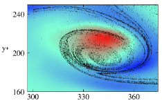
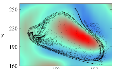
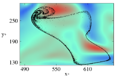
Figure 4: Time evolution of the floater cluster highlighted in Fig. 2(b). The cluster is examined following its Lagrangian path, with Eulerian coordinates in each snapshot changing accordingly. Floaters are hit by an upwelling (red region) at time $t^{+}\simeq 121$ (a), and scattered around at time $t^{+}\simeq 145$ (b). Eventually, they form a highly-concentrated filamentary pattern at time $t^{+}\simeq 193$ (c). This pattern exhibits strong time persistency and over-lives several surface-renewal events.

(a)                                     (b)

(c)

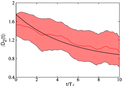
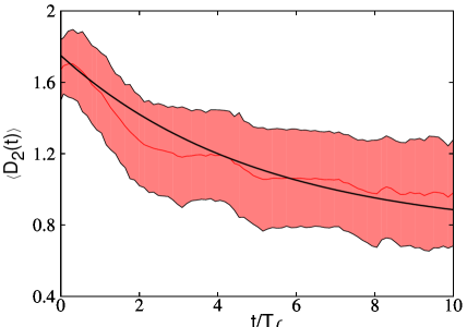
Figure 5: Time evolution of the cluster correlation dimension $\langle D_{2}(t)\rangle$ at the free surface. Panels: (a) $Re_{\tau}^{H}$; (b) $Re_{\tau}^{L}$. The red line in each panel shows the mean correlation dimension,$\langle D_{2}(t)\rangle$, the black line represents the estimate of $\langle D_{2}(t)\rangle$ yield by an exponentially-decaying fit:$\langle D_{2}(t)-D_{2}(\infty)\rangle\propto exp(-t/\alpha T_{\cal L})$ with $\alpha\simeq 5$ for both $Re_{\tau}^{H}$ and $Re_{\tau}^{L}$. The red area represents the standard deviation from $\langle D_{2}(t)\rangle$. Time is given as proportional to the Lagrangian integral timescale of the flow at the free-surface.

(a) $Re_{\tau}^{H}$

(b) $Re_{\tau}^{L}$

—— $\langle D_{2}(t)\rangle$

—— Exp. fit

$\blacksquare$ $\blacksquare$ $\blacksquare$ $\sigma_{\langle D_{2}(t)\rangle}$

—— $\langle D_{2}(t)\rangle$

—— Exp. fit

$\blacksquare$ $\blacksquare$ $\blacksquare$ $\sigma_{\langle D_{2}(t)\rangle}$

IV Conclusions and future development

The present study highlights the intermittent character of particle spatial distribution in free-surface turbulence. Intermittency is due buoyancy-driven clustering effects that are in turn connected to the formation of sources and sinks of fluid velocity generated by sub-surface upwelling and downwelling motions in the bulk of the sub-surface flow. At small time scales, the process of cluster formation is driven by the divergence of the flow field at the surface: Clusters evolve in time producing fractal-like surface patterns that can be characterized by their correlation dimension. Our results indicate that these patterns slowly relax towards a long-term distribution with exponential decay rate, requiring several Lagrangian integral fluid timescales. We remark here that, according to [10], [12], the surface-renewal timescale, which is usually employed to quantify interface scalar fluxes, is much smaller than the Lagrangian timescale and is thus inappropriate to quantify floater distribution dynamics.

Surface compressibility may play an important role in determining the motion of passive tracers like pollutants and nutrients but also the spreading rate of active ocean surfactants, such as phytoplankton [2]. Our findings provide useful indications to parameterize the relevant timescales characterizing dispersion of such species and, therefore, can assist in developing reliable predictive models [20].

References

• B. Eckhardt, and J. Schumacher, Phys. Rev. E. $\mathbf{64}$, 016314 (2001).

• J. R. Cressman, J. Davoudi, W. I. Goldburg, and J. Schumacher, New J. Phys. $\mathbf{6}$, 53 (2004).

• J. Larkin, M. M. Bandi, A. Pumir, and W. I. Goldburg, Phys. Rev. E $\mathbf{80}$, 066301 (2009).

• J. Larkin, W. I. Goldburg, and M. M. Bandi, Physica D $\mathbf{239}$, 1264 (2010).

• A. Soldati, and C. Marchioli, Int. J. Multiphase Flow $\mathbf{35}$, 827 (2009).

• Y. Pan, and S. Banerjee, Phys. Fluids $\mathbf{7}$, 1649 (1995).

• J. Ruiz, D. Macias, and F. Peters, Proc. Natl. Acad. Sci. USA 101, 17720 (2004).

• S. Komori, H. Ueda, F. Ogino, and T. Mizushina, Int. J. Heat Mass Transfer $\mathbf{25}$, 513 (1982).

• M. Rashidi, and S. Banerjee, Phys. Fluids $\mathbf{31}$, 2491 (1988).

• S. Komori, Y. Murakami, and H. Ueda, J. Fluid Mech. $\mathbf{203}$, 103 (1989).

• R. Nagaosa, and R. A. Handler, Phys. Fluids $\mathbf{15}$, 375 (2003).

• A. Kermani, H. R. Khakpour, L. Shen, and T. Igusa, J. Fluid Mech. $\mathbf{678}$, 379 (2011).

• R. Nagaosa, and R. A. Handler, AIChE J. $\mathbf{58}$, 3867 (2012).

• T. Sarpkaya, Annu. Rev. Fluid. Mech. $\mathbf{28}$, 83 (1996).

• S. Kumar, R. Gupta, and S. Banerjee, Phys. Fluids $\mathbf{10}$, 437 (1998).

• R. H. Kraichnan, Phys. Fluids $\mathbf{10}$, 1417 (1967).

• G. K. Batchelor, Phys. Fluids $\mathbf{233}$, 233 (1969).

• D. G. Dritschell, and B. Legras, Phys. Today $\mathbf{46}$, 44 (1993).

• P. Tabeling, Phys. Reports $\mathbf{362}$, 1 (2002).

• M. S. Spydell, and F. Feddersen, J. Fluid Mech. $\mathbf{691}$, 69 (2012).