On the magnetization of gamma-ray burst blast waves

Abstract

The origin of magnetic fields that permeate the blast waves of gamma-ray bursts (GRBs) is a long-standing problem. The present paper argues that in four GRBs revealing extended emission at $>100\,{\rm MeV}$, with follow-up in the radio, optical and X-ray domains at later times, this magnetization can be described as the partial decay of the micro-turbulence that is generated in the shock precursor. Assuming that the bulk of the extended emission $>100\,$MeV can be interpreted as synchrotron emission of shock-accelerated electrons, we model the multi-wavelength light curves of GRB 090902B, GRB 090323, GRB 090328 and GRB 110731A, using a simplified then a full synchrotron calculation with power-law-decaying micro-turbulence $\epsilon_{B}\,\propto\,t^{\alpha_{t}}$ ($t$ denotes the time since injection through the shock, in the comoving blast frame). We find that these models point to a consistent value of the decay exponent $-0.5\,\lesssim\,\alpha_{t}\,\lesssim\,-0.4$.

1 Introduction

In principle, the multi-wavelength light curves of gamma-ray bursts (GRBs) in the afterglow phase open a remarkable window on the physics of relativistic, weakly magnetized collisionless shock waves: these light curves are indeed thought to result from the synchrotron process of electrons accelerated at the external shock wave, so that their modelling leads to two microphysical parameters of importance: the fraction of shock dissipated energy stored in the suprathermal electron population, $\epsilon_{e}$, and in the self-generated electromagnetic turbulence, $\epsilon_{B}$.

From a theoretical point of view, one expects $\epsilon_{B}\,\sim\,0.1$ at the shock front (and $\epsilon_{e}\,\sim\,0.1$): the shock wave forms when a magnetic barrier on the ion skin depth scale $\,\sim\,c/\omega_{\rm pi}$ builds up through small-scale electromagnetic instabilities, up to the level at which it can deflect by an angle of the order of unity the incoming particles, which carry Lorentz factor $\gamma_{\rm sh}$ in the shock front frame; this demands $\epsilon_{B}\,\sim\,1/4$. This picture has been validated by high performance particle-in-cell (PIC) simulations (e.g. Spitkovsky 2008, Martins et al. 2009, Haugbølle 2011, Sironi & Spitkovsky 2011, 2013), and supported by theoretical arguments (e.g. Medvedev & Loeb 1999). However, on such small plasma scales, the micro-turbulence should decay rapidly behind the shock (e.g. Gruzinov & Waxman 1999), whereas early afterglow models of GRBs have pointed to finite, substantial values of $\epsilon_{B}$ on the (comoving) scale of the blast $\sim ct_{\rm dyn}$ [with $t_{\rm dyn}\,\sim\,r/(\gamma_{\rm b}c)$ the dynamical time-scale, $\gamma_{\rm b}$ the blast Lorentz factor], many orders of magnitude larger than the skin depth scale (e.g. Piran 2004, and references therein): $t_{\rm dyn}\omega_{\rm pi}\,\sim\,2\times 10^{7}\,E_{54}^{1/8}n_{0}^{3/8}t_{2}^{5/8}$. Nevertheless, the decay of Weibel turbulence has been observed in dedicated numerical experiments (Chang et al. 2008, Keshet et al. 2009, Medvedev et al. 2011), although admittedly, such simulations can probe only a small fraction of a GRB dynamical time-scale.

The detection of extended high energy emission $>100\,$MeV by the Fermi-LAT instrument in several GRBs has brought in new constraints in this picture. Most notably, the synchrotron model of this emission has pointed to values of $\epsilon_{B}$ much smaller than unity in an adiabatic scenario (Kumar & Barniol-Duran 2009, 2010, Barniol-Duran & Kumar 2011, He et al. 2011, Liu & Wang 2011). Kumar & Barniol-Duran (2009) have noted that the magnetic field in which the electrons radiate corresponds to a strength $\sim 10\,\mu$G in the upstream frame, before shock compression; they therefore interpret this magnetic field as the simple shock compression of the interstellar field. However, the fact that the inferred $\epsilon_{B}$ lies a few orders of magnitude above the interstellar magnetization level $\sim 10^{-9}$ rather suggests that the electrons radiate in a partially decayed micro-turbulence (Lemoine 2013); theoretically, such a picture could reconcile the results of PIC simulations with the observational determinations of $\epsilon_{B}$.

In the present work, we push forward this idea and put it to the test by considering the multi-wavelength light curves of four GRBs observed in radio, optical, X-ray and GeV in the framework of a decaying micro-turbulence afterglow scenario. We show that these four bursts point to a consistent value of the decay index $-0.5\,\lesssim\,\alpha_{t}\,\lesssim\,-0.4$, if one assumes that $\epsilon_{B}\,\propto\,t^{\alpha_{t}}$, with $t$ the time since injection of the plasma through the shock, as measured in the comoving blast frame, and $\epsilon_{B}\,\sim\,0.01$ at $t\,=\,100\omega_{\rm pi}^{-1}$, as observed in PIC simulations. To do so, we first present a simplified model of this afterglow (Section 2), with two radiating zones, in each of which one can use the standard afterglow model (e.g. Sari et al. 1998); then we provide a detailed treatment of the power-law decay of the micro-turbulence (Section 2.3), improving on Lemoine (2013). We confront our findings to previous results in Section 3.

2 Afterglow model

2.1 General considerations

The calculation of the synchrotron spectrum of a relativistic blast wave with decaying micro-turbulence can be approximated (and much simplified) by noting that photons in different frequency bands have been emitted by electrons of different Lorentz factors, which cool at different times since their injection, hence in regions of different magnetic field strengths. In this approximate treatment, one can therefore use the standard homogeneous afterglow model for each frequency band, allowing for a possibly different $\epsilon_{B}$ in each band. When compared to the detailed calculations with decaying micro-turbulence, one finds that the above provides a reasonable approximation, provided the decay index $\alpha_{t}\,\gtrsim\,-1$. We make this approximation in the present work and justify it a posteriori.

According to the above picture, one should take a similar $\epsilon_{B-}$ for all frequencies $\nu\,<\,\nu_{\rm c}$ that correspond to Lorentz factors $\gamma\,<\,\gamma_{\rm c}$ such that the cooling time-scale exceeds the dynamical time-scale, $t_{\rm cool}(\gamma)\,\gtrsim\,t_{\rm dyn}$. Such particles indeed radiate most of their synchrotron energy in the same region, at the back of the blast. For GRB afterglows with extended $>100\,{\rm MeV}$ emission, in which we are interested here, this concerns the radio and optical range, and possibly the X-ray range at late times. For those frequencies, one can therefore use the standard homogeneous approximation of slowly cooling particles for the calculation of $F_{\nu}$.

At the other extreme, GeV photons are likely produced in a region of strong $\epsilon_{B}$, due to the short cooling time-scale of the emitting parent electrons. The large Lorentz factors also generally imply that inverse Compton losses are negligible in this frequency range due to Klein-Nishina (KN) suppression, although this should be verified on a case-to-case basis. Given these assumptions, the expected flux depends on the ejecta kinetic energy $E$ and $\epsilon_{e}$, but very little on the other parameters, $\epsilon_{B}$ in particular. Indeed, the energy radiated in the GeV range corresponds to $\sim(\gamma_{8}/\gamma_{\rm min})^{2-s}$ times the blast energy stored in the electron distribution $\propto\,\epsilon_{e}E$, where $\gamma_{8}$ denotes the minimum Lorentz factor of electrons radiating at $>100\,$MeV. It is easy to see that $\gamma_{8}/\gamma_{\rm min}\,\propto\,\epsilon_{B}^{-1/4}$, so that the residual dependence of $F_{\nu}(>100\,{\rm MeV})$ on $\epsilon_{B}$ is quite small. As inverse Compton losses can be neglected at those energies, the flux does not depend either on the external density $n$. As already noted in Kumar & Barniol-Duran (2009), the flux density $F_{\nu}(>100\,{\rm MeV})$ provides a unique constraint on the model parameters, all the more so in the present case of decaying micro-turbulence.

The application of the above simple algorithm allows us to evaluate the parameters of the afterglow in the framework of the standard model. One outcome of this analysis is the measurement of $\epsilon_{B-}$, which represents the value of $\epsilon_{B}$ at the back of the blast, through the modelling of the radio, optical and X-ray flux. Since the dynamical time-scale is determined by the standard parameters of the blast, one can constrain directly the exponent of power law decay $\alpha_{t}$:

$$\alpha_{t}\,=\,\frac{\log\left[\epsilon_{B-}/\epsilon_{B+}\right]}{\log\left[t_{\rm dyn}/\tau_{\delta B}\right]}\ ,$$ (1)

up to logarithmic corrections dependent on $\tau_{\delta B}\,\sim\,100\omega_{\rm pi}^{-1}$, the time scale beyond which turbulence starts to decay and $\epsilon_{B+}\,\sim\,0.01$, the value of the micro-turbulence close to the shock front, both of which are constrained by PIC simulations.

Care must be taken in the course of this exercise, because for low $\epsilon_{B-}$, the Compton parameter at the cooling frequency $Y_{\rm c}\,\gg\,1$, and KN suppression of the inverse Compton process may be efficient in the X-ray range at late times. The magnitude of KN suppression at frequency $\nu$ can be quantified through the following equation:

$$\Upsilon_{\rm KN}(\nu) \,\equiv\, \frac{h\nu_{\rm c}(1+z)}{\gamma_{\rm b}}\frac{\gamma(\nu)}{m_{e}c^{2}}$$ (2)

$$\,\simeq\, 50\,E_{54}^{1/4}t_{5}^{1.36}A_{35}^{-2.10}\epsilon_{B-,-5}^{-0.80}\epsilon_{e,-1}^{-1.16}\nu_{17.38}^{1/2}\ ,$$

where $\gamma(\nu)$ denotes the Lorentz factor of electrons whose (observer frame) synchrotron peak frequency equals $\nu$. For the numerical values, we have assumed a wind profile of external density $n=10^{35}A_{35}\,r^{-2}\,$cm^-3, an electron spectral index $p=2.2$, $\nu\,>\,\nu_{\rm c}$ with $Y_{\rm c}$ given by Sari & Esin (2001) in the slow cooling regime, and $z=1$. $\Upsilon_{\rm KN}\,>\,1$ at X-ray frequencies means that KN suppression of the inverse Compton cooling is efficient and cannot be ignored.

The optical and radio data of the following light curves always lie below $\nu_{\rm c}$, in which case the Compton parameter does not depend on the electron Lorentz factor, $Y(\gamma)\,=\,Y_{\rm c}$, the Compton parameter at $\gamma_{\rm c}$ (or equivalently, $\nu_{\rm c}$). In contrast, at GeV energies KN suppression is so efficient that the Compton parameter $Y_{>100\,\rm MeV}\,\ll\,1$ (e.g. Wang et al. 2010, Liu & Wang 2011). Therefore, inverse Compton losses with substantial KN suppression, which modify the synchrotron spectrum (e.g. Nakar et al. 2009, Wang et al. 2010), concern only the X-ray domain at late times.

We therefore proceed as follows. We first search a solution assuming $\Upsilon_{\rm KN}\,<\,1$ in the X-ray range, with possibly large $Y_{\rm c}$. We then compute $\Upsilon_{\rm KN}$, and if $\Upsilon_{\rm KN}\,>\,1$, we look for another solution in which we take into account the effect of KN suppression in the X-ray domain, following Li & Waxman (2006), Nakar et al. (2009) and Wang et al. (2010). In particular, we solve the following equations for the cooling Lorentz factor $\gamma_{\rm c}$ and Compton parameter $Y_{\rm c}$ at the cooling frequency:

$$\left(1+Y_{\rm c}\right)\gamma_{\rm c} \,=\, \gamma_{\rm c,syn}\ ,$$

$$Y_{\rm c}\left(1+Y_{\rm c}\right) \,=\, \frac{\epsilon_{e}}{\epsilon_{B-}}\left(\frac{\gamma_{\rm c}}{\gamma_{\rm min}}\right)^{2-p}\,\left[{\rm min}\left(1,\frac{\hat{\gamma}_{\rm c}}{\gamma_{\rm c}}\right)\right]^{(3-p)/2}\ ,$$ (3)

with (see Nakar et al. 2009, Wang et al. 2010)

$$\gamma_{\rm c,syn}\,\equiv\,\left.\gamma_{\rm c}\right|_{Y_{\rm c}\,\rightarrow\,0}\ ,\quad\hat{\gamma}_{\rm c}\,\equiv\,\frac{\gamma_{\rm b}m_{e}c^{2}}{h\nu_{\rm c}(1+z)}\ .$$ (4)

We neglect more extreme cases in which the electron interacts with low-frequency bands of the synchrotron spectrum, below $\nu_{\rm min}$. We then consider a synchrotron spectrum in the slow cooling phase (generic in the cases that we study) $F_{\nu}\,\propto\,t_{\rm obs}^{-\alpha}\nu^{-\beta}$ with $\beta\,=\,3(p-1)/4$ above $\nu_{\rm c}$ instead of $\beta\,=\,p/2$ when $\Upsilon_{\rm KN}\,<\,1$. We then verify a posteriori that the Compton parameter in the X-ray range $Y_{\rm X}\,>\,1$, if the X-ray range is fitted with this modified spectrum. In the GeV range, we always find $Y_{>100\,{\rm MeV}}\,\ll\,1$ due to KN suppression; therefore, we keep $\beta\,=\,p/2$ in that range. In Section 2.3, we incorporate the influence of decaying micro-turbulence, which modifies further the time and frequency dependencies of the synchrotron afterglow flux.

Finally, let us stress that while we assume that the bulk of the emission at energy $>100\,{\rm MeV}$ originates from synchrotron radiation, we do not exclude that a fraction of the highest energy photons are actually produced by inverse Compton processes. In (homogeneous) small-scale turbulence, the high energy electrons suffer only small angular deflections as they cross a coherence length of the turbulence, so that their residence time (hence the acceleration time) becomes substantially larger than the gyrotime, which sets the residence time in a large-scale field (although advection impedes acceleration in large-scale turbulence; see Lemoine, Pelletier & Revenu 2006). Hence, in small-scale turbulence peaked on a wavelength $\lambda\,=\,10\,c/\omega_{\rm pi}$ with $\epsilon_{B+}\,=\,0.01$, the maximum synchrotron photon energy falls to $1$-$3\,$GeV at an observed time of $100\,$s for generic GRB afterglow parameters, see e.g. Kirk & Reville (2010), Bykov et al. (2012), Plotnikov, Pelletier & Lemoine (2013), Lemoine (2013) and Wang, Liu & Lemoine (2013), compared to a few tens of GeV for the ideal case of Bohm acceleration on a gyrotime, e.g. Lyutikov (2010). In a decaying micro-turbulence, the maximum photon energy does not depart much from the value for homogeneous small-scale turbulence with $\epsilon_{B+}\,=\,0.01$, see Lemoine (2013), because the highest energy electrons cool on a relatively short time-scale, in regions of strong $\epsilon_{B}$ and at the same time interact with modes of wavelength larger than $\lambda$. For instance, a value of $\simeq\,2\,$GeV is derived at $100\,$s assuming that the minimum scale of the turbulence $\lambda=10\,c/\omega_{\rm pi}$ for a decay index $\alpha_{t}=-0.5$ and a damping time of the turbulent modes $\tau\propto\lambda^{2}$. In this context, one should thus expect that photons of energy $\gtrsim\,10\,$GeV do not originate from synchrotron radiation, but from inverse Compton interactions, see Wang, Liu & Lemoine (2013). However, the bulk of the emission $>100\,$MeV can be produced by synchrotron radiation and we make this assumption in the present work. The energy interval $100\,{\rm MeV}-10\,{\rm GeV}$ indeed represents the bulk of the emission for the GRBs seen with extended emission, because their photon indices are $\simeq-2$, see Ackermann et al. (2013b). Of course, we verify a posteriori that the predicted synchrotron self-Compton (SSC) contribution does not exceed the synchrotron flux at energies $>100\,{\rm MeV}$.

2.2 Application to four Fermi-LAT GRBs

We now discuss the application of this exercise to four GRBs observed in the radio, optical, X-ray and GeV range: GRB 090902B, GRB 090323, GRB 090328 and GRB 110731A. We select them because four observational constraints (corresponding to the four frequency bands) are required to determine unambiguously the four parameters: $\epsilon_{e}$, $\epsilon_{B-}$, $E$ and $n$. These four bursts have been discussed in the literature: the first three by Cenko et al. (2011) and the last one by Ackermann et al. (2013a). We will compare our results to these studies in Sec. 3.

2.2.1 GRB 090902B

We assume in the following $p=2.3$, as suggested by the previous analyses of Cenko et al. (2011), Kumar & Barniol-Duran (2010), Barniol-Duran & Kumar (2011) and Liu & Wang (2011), and $k=0$ (constant density profile). The flux density at $100\,$MeV reads

$$F_{\nu}\,\simeq\,6\times 10^{-9}\,{\rm Jy}\,E_{54}^{1.05}\epsilon_{B+,-2}^{0.05}\epsilon_{e,-1}^{1.2}t_{2}^{-1.15}\ ,$$ (5)

so that its measured value $\simeq\,0.22\,\mu$Jy at a time $t_{\rm obs}\,=\,50\,$s leads to

$$E_{54}\,\simeq\,11.1\,\epsilon_{e,-1}^{-1.21}\ .$$ (6)

We have discarded the dependence on the Compton parameter $Y_{>100\,{\rm MeV}}\,\ll\,1$ and on $\epsilon_{B+}$, since we assume that the value of $\epsilon_{B+}$ that would enter this equation is close to $0.01$, and its exponent is small.

For the optical range in the $R$ band at $\nu_{\rm opt}$, we assume $\nu_{\rm min}\,<\,\nu_{\rm opt}\,<\,\nu_{\rm c}$ at $t_{\rm obs}\,=\,65\,000\,$s, with flux density $1.8\times 10^{-5}\,$Jy. Therefore, the optical flux

$$F_{\nu}\,\simeq\,0.088\,{\rm Jy}\,E_{54}^{1.3}n_{-2}^{0.5}\epsilon_{B-,-2}^{0.8}\epsilon_{e,-1}^{1.2}t_{2}^{-0.9}$$ (7)

leads to the constraint, once equation 6 has been taken into account:

$$\epsilon_{B-,-2}\,\simeq\,4.1\times 10^{-5}\,\epsilon_{e,-1}^{0.37}n_{0}^{-0.61}\ .$$ (8)

Quite interestingly, these two GeV and optical determinations lead by themselves to very low values of $\epsilon_{B-}$, provided that $\epsilon_{e,-1}$ and $n_{0}$ do not differ strongly from unity. The radio flux at $\nu_{\rm rad}=8.5\,$GHz lies in the range of $\nu_{\rm rad}\,<\,\nu_{\rm min}\,<\,\nu_{\rm c}$ at $t_{\rm obs}\,\sim\,10^{5}\,$s, so that

$$F_{\nu}\,\simeq\,4.2\times 10^{-5}\,{\rm Jy}\,E_{54}^{5/6}\epsilon_{B-,-2}^{1/3}n_{-2}^{1/2}t_{2}^{1/2}\epsilon_{e,-1}^{-2/3}\ ,$$ (9)

to be matched to $F_{\nu}\,\sim\,1.3\times 10^{-4}\,$Jy at $4.8\times 10^{5}\,$s; when combined with the above equations (6) and (8), this implies

$$n_{0}\,\simeq\,2.5\times 10^{-6}\,\epsilon_{e,-1}^{5.21}\ .$$ (10)

The decay rate in the X-ray range at $t_{\rm obs}\,>\,10^{5}\,$s suggests that $\nu_{\rm c}<\nu$ (see Liu & Wang 2011), which therefore brings in complementary constraints relatively to the optical and radio domains. In principle, one should allow for a different $\epsilon_{B}$ parameter in the region in which X-rays are produced; here, we make however the approximation that this $\epsilon_{B}\,\sim\,\epsilon_{B-}$. In Section 2.3, we compute the afterglow allowing for the dependence of $\epsilon_{B}$ on location, thus correcting this approximation.

If one first neglects KN suppression in the X-ray range, one is led to a solution with $\epsilon_{e,-1}\,\sim\,2.7$, but with $\Upsilon_{\rm KN}\,\sim\,350$ at times $5\times 10^{5}\,$s, so that one needs to include the KN suppression. Following the above algorithm, and using the X-ray flux measurement between $0.3\,$ and $10\,$keV of $2.2\times 10^{-13}\,$erg/cm²/s at $5.2\times 10^{5}\,$s, with $\nu_{\rm X}>\nu_{\rm c}$, one derives $\epsilon_{e}$, hence the parameter set

$$\epsilon_{e} \,\simeq\, 0.46\ ,\quad E\,\simeq\,1.8\times 10^{54}\,{\rm erg}\ ,$$

$$\epsilon_{B-} \,\simeq\, 1.5\times 10^{-5}\ ,\quad n\,\simeq\,7.0\times 10^{-3}\,{\rm cm}^{-3}\ .$$ (11)

We also note that $\nu_{\rm c}\,\simeq\,8.2\times 10^{16}\,{\rm Hz}$ at $5.2\times 10^{5}\,$s, $Y_{\rm c}\,\sim\,27$, just as $\nu_{\rm rad}\,<\,\nu_{\rm min}$ and $\nu_{\rm min}\,<\,\nu_{\rm opt}\,<\,\nu_{\rm c}$ at the respective times; the solution is therefore consistent.

This light curve therefore indicates a low value for $\epsilon_{B-}$, corresponding to a decay exponent

$$\alpha_{t}\,\simeq\,-0.44\pm 0.10\ ,$$ (12)

assuming $\epsilon_{B+}=0.01$ at $t\,=\,100\,\omega_{\rm pi}^{-1}$. We used the value of $t_{\rm dyn}$ at time $10^{5}\,$s, at which the predicted spectrum has been normalized to the optical and radio data. We derive the uncertainty on $\alpha_{t}$ by propagating conservative estimates of the uncertainties in the value of $p$, of $k$ and the statistical errors of the data used for normalization. As $p$ goes from $2.1$ to $2.5$, $\alpha_{t}$ changes from $-0.36$ to $-0.48$. If $k=2$ instead of $0$, one finds $\alpha_{t}=-0.51$ . For this burst, scintillation in the radio range provides the largest source of uncertainty, leading to a conservative factor $\sim 3$ uncertainty on the flux, which in turn leads to an error $\simeq\,0.03$ on $\alpha_{t}$. In total, we estimate the uncertainty $\Delta\alpha_{t}\,\simeq\,0.10$.

2.2.2 GRB 090323

We repeat the same exercise with GRB 090323, which has been observed at $>100\,$MeV up to a few hundred seconds, and in the X-ray, optical and radio domains, short of a day onwards. In what follows, we use $p=2.5$, slightly smaller than the value found by Cenko et al. (2011) in their best fit, and $k=2$. The $>100\,$MeV flux is normalized to $\phi(>100\,{\rm MeV})\,=\,1.5\times 10^{-5}\,$photon cm^-2 s^-1 at $350\,$s, leading to

$$E_{54}\,\simeq\,27.7\,\epsilon_{e,-1}^{-1.33}\ ,$$ (13)

while the optical flux is normalized to $1.3\times 10^{-5}\,$Jy at $1.6\times 10^{5}\,$s, assuming $\nu_{\rm min}\,<\,\nu_{\rm opt}\,<\,\nu_{\rm c}$, leading to

$$\epsilon_{B,-2}\,\simeq\,2.1\times 10^{-3}A_{35}^{-1.14}\epsilon_{e,-1}^{-0.38}\ ,$$ (14)

once equation (13) has been taken into account; then, normalization to the radio flux $2.\times 10^{-4}$ Jy at $4.3\times 10^{5}\,$s with $\nu_{\rm rad}\,<\,\nu_{\rm min}\,<\,\nu_{\rm c}$ leads to

$$A_{35}\,\simeq\,0.98\,\epsilon_{e,-1}^{2}\ .$$ (15)

Here as well, note that the radio, optical and GeV constraints lead to a very low value for $\epsilon_{B}$, if one assumes a parameter $\epsilon_{e}$ close to the value inferred in PIC simulations, $\epsilon_{e,-1}\,\sim\,1$. To account for the X-ray flux, $\,\simeq\,10^{-13}\,$erg/cm²/s at $2.5\times 10^{5}\,$s, it is here as well necessary to consider the influence of KN suppression, which eventually leads to

$$\epsilon_{e} \,\simeq\, 0.25\ ,\quad E\,\simeq\,8.1\times 10^{54}\,{\rm erg}\ ,$$

$$\epsilon_{B-} \,\simeq\, 1.8\times 10^{-6}\ ,\quad A\,\simeq\,6.1\times 10^{35}\,{\rm cm}^{-1}\ .$$ (16)

This corresponds to a decay index

$$\alpha_{t}\,\simeq\,-0.54\pm 0.09\ ,$$ (17)

where the error accounts for a factor of 2 uncertainty on the GeV flux (leading to $\pm 0.06$ on $\alpha_{t}$), a factor of 2 uncertainty on the radio determination (leading to $\pm 0.03$) and an uncertainty $\Delta p=\pm 0.2$ (leading to $\pm 0.04$); finally, if $k=0$ instead of $k=2$, one finds $\alpha_{t}=-0.50$.

2.2.3 GRB 090328

The multi-wavelength light curve for this burst is rather similar to that of GRB 090323, and we proceed analogously. Using a $>100\,$MeV flux of $2.9\times 10^{-6}$ photon cm^-2 s^-1 at $1.1\times 10^{3}\,$s, we obtain

$$E_{54}\,\simeq\,2.1\,\epsilon_{e,-1}^{-1.33}\ ,$$ (18)

while the optical flux is normalized to $3\times 10^{-5}\,$Jy at $0.6\times 10^{5}\,$s (with $\nu_{\rm min}\,<\,\nu_{\rm opt}\,<\,\nu_{\rm c}$), leading to

$$\epsilon_{B,-2}\,\simeq\,1.5\times 10^{-3}A_{35}^{-1.14}\epsilon_{e,-1}^{-0.38}\ .$$ (19)

Normalization to the radio flux $6\times 10^{-4}$ Jy at $3\times 10^{5}\,$s ($\nu_{\rm rad}\,<\,\nu_{\rm min}\,<\,\nu_{\rm c}$) leads to

$$A_{35}\,\simeq\,0.4\,\epsilon_{e,-1}^{2}\ .$$ (20)

The X-ray flux is normalized to $2.7\times 10^{-12}\,$erg/cm²/s at $0.63\times 10^{5}\,$s, in the KN regime, which leads to $\epsilon_{e}$, hence

$$\epsilon_{e} \,\simeq\, 0.19\ ,\quad E\,\simeq\,0.88\times 10^{54}\,{\rm erg}\ ,$$

$$\epsilon_{B-} \,\simeq\, 7.6\times 10^{-6}\ ,\quad A\,\simeq\,1.5\times 10^{35}\,{\rm cm}^{-1}\ .$$ (21)

This corresponds to a decay index

$$\alpha_{t}\,\simeq\,-0.46\pm 0.11\ ,$$ (22)

at time $10^{5}\,$s. The error accounts for a factor of 2 uncertainty on the GeV flux (leading to $\pm 0.06$ on $\alpha_{t}$), a factor of 2 uncertainty on the radio determination (leading to $\pm 0.02$) and an uncertainty $\Delta p=\pm 0.2$ (leading to $\pm 0.08$); finally, if $k=0$ instead of $k=2$, one finds $\alpha_{t}=-0.42$.

2.2.4 GRB 110731A

This burst presents the most comprehensive multi-wavelength follow-up of a LAT burst with extended emission at $>100\,$MeV; X-ray and optical start short of $100\,$s, while $>100\,$MeV emission is still ongoing. Unfortunately, there are no radio detections for this burst, only an upper limit of $5\times 10^{-5}\,$Jy at $0.58\times 10^{5}\,$s (Zauderer et al. 2011). Nevertheless, one can obtain strong constraints on $\epsilon_{B}$, by noting that the optical frequency $\nu_{\rm opt}=5.5\times 10^{14}\,$Hz must satisfy $\nu_{\rm opt}\,>\,\nu_{\rm min}$ at $t_{\rm obs}=100\,$s, because the optical decays as a power law with index $\alpha\,\simeq\,1.37$; if the opposite inequality were to hold at this time, one would rather observe $\alpha=0$ for slow cooling, or $\alpha=1/4$ for fast cooling. We thus write $\nu_{\rm min}\,=\,C_{\nu}\,\nu_{\rm opt}$ with $C_{\nu}\,>\,1$ at $100\,$s, which imposes

$$\epsilon_{B,-2}\,\simeq\,5.1\times 10^{-4}C_{\nu}^{-2}E_{54}^{-1}\epsilon_{e,-1}^{-4}\ .$$ (23)

Here and in the following, we assume $p=2.1$ and $k=2$. Given that $C_{\nu}>1$, this obviously restricts $\epsilon_{B}$ to very low values, if $E$ and $\epsilon_{e}$ take close to standard values. We next normalize the predicted $F_{\nu}$ to the observed optical flux density $\,\simeq\,3.5\times 10^{-4}\,$Jy at $1100\,$s, assuming $\nu_{\rm min}\,<\,\nu_{\rm opt}\,<\,\nu_{\rm c}$ (verified a posteriori), which leads to

$$A_{35}\,\simeq\,1.5\,C_{\nu}^{1.55}\epsilon_{e,-1}^{2}\ .$$ (24)

The above two conditions imply a radio flux which is a factor of $\simeq 4.1$ in excess of the observational upper bound; this remains reasonable given the amount of scintillation typically expected at this time, and seen in the other bursts. We then use the $>100\,$MeV flux, $\phi(>100\,{\rm MeV})\,\simeq\,8.4\times 10^{-5}$ photon cm^-2 s^-1 at $26\,$s, to derive

$$E_{54}\,\simeq\,2.5\,\epsilon_{e,-1}^{-1.07}\ ,$$ (25)

and finally the X-ray flux, $2\times 10^{-9}\,$erg/cm²/s at $100\,$s, assuming $\nu_{\rm c}<\nu_{\rm X}$. For this burst, KN suppression is not effective at such an early time and it can be neglected in the normalization; however, $\nu_{\rm c}$ is eventually found to be close to $1\,$keV, which makes this solution only approximate. In Section 2.3, we derive a better fit by adjusting by hand the missing parameter $\epsilon_{e,-1}$ under the above constraints. Modulo this small uncertainty, the X-ray flux leads to

$$\epsilon_{e} \,\simeq\, 0.021\,C_{\nu}^{-0.50}\ ,\quad E\,\simeq\,13.\times 10^{54}\,C_{\nu}^{0.54}\,{\rm erg}\ ,$$

$$\epsilon_{B-} \,\simeq\, 1.9\times 10^{-4}\,C_{\nu}^{-0.53}\ ,\quad A\,\simeq\,0.068\times 10^{35}\,C_{\nu}^{0.54}\,{\rm cm}^{-1}\ .$$

This implies a decay index

$$\alpha_{t}\,\simeq\,-0.35\frac{1+0.51\ln C_{\nu}}{1+0.10\ln C_{\nu}}\ ,$$ (27)

at $t_{\rm obs}=1100\,$s. Assuming $C_{\nu}=1$, we estimate a conservative uncertainty on $\alpha_{t}$ to be $\Delta\alpha_{t}\,\simeq\,\pm 0.2$ given that a factor of $2$ uncertainty on the GeV flux leads to an error $\pm 0.10$, $p=2.01$ leads to $\alpha_{t}=-0.14$ while $p=2.3$ leads to $\alpha_{t}=-0.53$. Note that the light curves leave very little ambiguity on the density profile (Ackermann et al. 2013); therefore, we do not consider $k=0$.

2.3 Multi-wavelength light curves in a decaying turbulence

We now include the effect of decaying micro-turbulence. The changing magnetic field modifies the spectral shape of electrons with $\gamma>\gamma_{\rm c}$, as well as the characteristic frequencies and their evolution in time (Lemoine 2013). With respect to the previous two-zone slow-cooling model, most of the difference concerns the X-ray domain, which lies above $\nu_{\rm c}$. The spectrum is computed as follows.

At frequencies $<\nu_{\rm c}$, the standard synchrotron spectrum holds, although the magnetic field value should be taken as the partially decayed micro-turbulent value at the back of the blast, which evolves in time:

$$\delta B_{-}\,\simeq\,\delta B_{+}\,\left(t_{\rm dyn}/\tau_{\delta B}\right)^{\alpha_{t}/2}\,\propto\,\epsilon_{B+}^{1/2}\,t_{\rm obs}^{(\alpha_{t}-6)/8}\ .$$ (28)

Of course, one recovers the standard time evolution in the limit $\alpha_{t}\,\rightarrow\,0$.

At frequencies $\nu_{\rm c}\,<\,\nu\,<\,\hat{\nu}_{\rm c}$, i.e. if $\nu_{\rm c}\,<\,\hat{\nu}_{\rm c}$ ($\hat{\nu}_{\rm c}$ designing the synchrotron peak frequency associated with $\hat{\gamma}_{\rm c}$), KN suppression is ineffective, $\Upsilon_{\rm KN}(\nu)<1$; therefore, the electrons cool in a uniform radiation background, but radiate their synchrotron flux in a changing magnetic field, all along their cooling history. This leads to a synchrotron spectral index

$$\beta\,=\,\frac{p+\alpha_{t}/2}{2-\alpha_{t}/2}\quad\left[\nu\,>\nu_{\rm c},\ ,\Upsilon_{\rm KN}(\nu)\,<\,1\right]\ ,$$ (29)

see the Appendix of Lemoine (2013), Sec. A3.

To account for the influence of KN suppressed inverse Compton losses at frequencies $\nu\,>\,{\rm max}\left(\nu_{\rm c}\ ,\,\hat{\nu}_{\rm c}\right)$, we proceed as follows. We first solve for $\gamma_{\rm c}$ and $Y_{\rm c}$ as in equations 3 and 4, using however a value $\delta B_{-}$ for the magnetic field at the back of the blast. We then solve for the cooling history $\gamma_{e}(t)$ of an electron with initial Lorentz factor (meaning at the shock front, $t$ representing the comoving since acceleration at the shock) $\gamma_{e,0}\,>\,\gamma_{\rm c}$, considering that if $\Upsilon_{\rm KN}(\nu)\,>\,1$, this electron interacts with a radiation field of energy density $Y(\gamma_{e})\delta B_{-}^{2}/(8\pi)$, characterized by the Lorentz factor dependent Compton parameter $Y(\gamma_{e})$ (e.g. Li & Waxman 2006, Nakar et al. 2009, Wang et al. 2010):

$$Y(\gamma_{e})\,\simeq\,Y_{\rm c}\,\left(\frac{\gamma_{e}}{\gamma_{\rm c}}\right)^{(p-3)/2}\ ,$$ (30)

assuming $\hat{\gamma}_{\rm c}\,<\,\gamma_{\rm c}\,<\,\gamma_{e}$. Here as well, we can neglect extreme cases in which the electron interacts with the low-frequency bands of the spectrum, below $\nu_{\rm min}$. Solving for the cooling history in this radiation field, one determines a cooling time-scale $t_{\rm cool}(\gamma_{e,0})\,\simeq\,t_{\rm dyn}(\gamma_{e,0}/\gamma_{\rm c})^{-(p-1)/2}$, and $\gamma_{e}(t)\,\simeq\,\gamma_{\rm c}(t/t_{\rm dyn})^{-2/(p-1)}$ for $t\,\gg\,t_{\rm cool}(\gamma_{e,0})$. Following Lemoine (2013), we then calculate the individual electron synchrotron contribution, by integrating the synchrotron power $\propto\,\gamma_{e}^{2}(t)\delta B^{2}(t)$ over this cooling history; then we evaluate the contribution of the electron population by folding the latter result over the injection distribution function of electron Lorentz factors. This leads to a synchrotron spectral index

$$\beta\,=\,\frac{3(p-1)}{4}\frac{1+\alpha_{t}/6}{1-\alpha_{t}(p-1)/8}\quad\left[\nu\,>\nu_{\rm c},\ ,\Upsilon_{\rm KN}(\nu)\,>\,1\right]\ ,$$ (31)

which tends to $3(p-1)/4$ as it should when $\alpha_{t}\rightarrow 0$ (non-decaying turbulence).

Finally, at $>100\,$MeV, we assume that inverse Compton losses are negligible; hence, we use the above $\beta=(p+\alpha_{t}/2)/(2-\alpha_{t}/2)$. This slight change of slope, as compared to the two-zone determinations, implies slightly different parameter values. The final estimates are given in the captions of Figs. 1, 2, 3 and  4, which present the models of these multi-wavelength light curves.

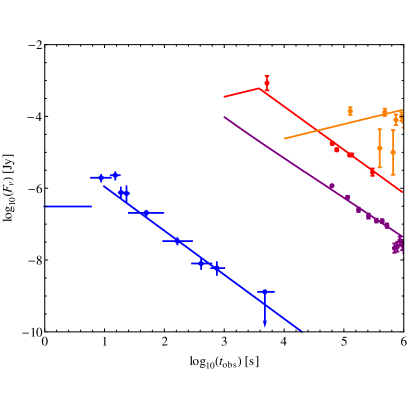
Figure 1: Multi-wavelength light curve for GRB 090902B; orange: radio flux density, red: optical $R$-band flux density, purple: X-ray flux $\int_{0.3\,{\rm keV}/h}^{10\,{\rm keV}/h}F_{\nu}\,{\rm d}\nu/\left(2.4\times 10^{17}\,{\rm Hz}\right)$, blue: spectral flux density $F_{\nu}$ at $2.4\times 10^{22}\,$Hz; parameter values: $E\,=\,1.6\times 10^{54}\,$ergs, $n=0.012\,$cm^-3, $\epsilon_{e}=0.50$, $p=2.3$, $k=0$ and $\alpha_{t}=-0.45$. Data taken from Cenko et al. (2011) and Abdo et al. (2009) and the Swift XRT repository data base (Evans et al. 2007, 2009).

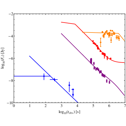
Figure 2: Same as Fig. 1, for GRB 090323, except that the blue data indicates the $>100\,{\rm MeV}$ flux $\int_{100\,{\rm MeV}/h}F_{\nu}\,{\rm d}\ln\nu$. Parameter values: $E\,=\,5.4\times 10^{54}\,$ergs, $A=8.4\times 10^{35}\,$cm^-1, $\epsilon_{e}=0.29$, $p=2.5$, $k=2$ and $\alpha_{t}=-0.54$. Data taken from Cenko et al. (2011), Piron et al. (2011) and the Swift XRT repository data base (Evans et al. 2007, 2009); a constant $R$-band flux of $4\times 10^{-7}\,$Jy models the host galaxy emission.

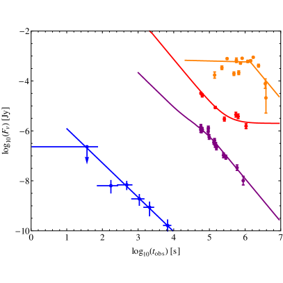
Figure 3: Same as Fig. 2, for GRB 090328 (using $U$-band optical data). Parameter values: $E\,=\,0.73\times 10^{54}\,$ergs, $A=1.5\times 10^{35}\,$cm^-1, $\epsilon_{e}=0.18$, $p=2.5$, $k=2$ and $\alpha_{t}=-0.45$. Data taken from Cenko et al. (2011), Piron et al. (2011) and the Swift XRT repository data base (Evans et al. 2007, 2009); a constant $R$-band flux of $2\times 10^{-6}\,$Jy models the host galaxy emission.

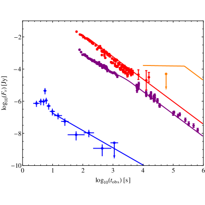
Figure 4: Same as Fig. 2, for GRB 110731A with in the optical range: UVOT $v$-band optical data, UVOT $w$-band data scaled to the $v$-band data, MoA $I$- and $V$-band data. Parameter values: $E\,=\,6.7\times 10^{54}\,$ergs, $A=0.15\times 10^{35}\,$cm^-1, $\epsilon_{e}=0.035$, $p=2.1$, $k=2$ and $\alpha_{t}=-0.38$. Data taken from Ackermann et al. (2013a) and the Swift XRT repository data base (Evans et al. 2007, 2009).

We have not attempted to obtain least-squares fits to these multi-wavelength light curves, rather we have used the normalization of the flux at several data points, as discussed in the previous sections, derived the parameters, then plotted the predicted multi-wavelength light curves. We have also neglected the possibility of significant extinction in the optical domain, which could improve the quality of the fit for GRB 110731A in particular. Moreover, our numerical code computes the light curves for a decelerating blast wave; it does not account for the initial ballistic stage, and neither does it account for sideways expansion beyond jet break. We have chosen to plot the $>100\,{\rm MeV}$ lightcurve assuming deceleration of the blast beyond $10\,$s, which corresponds to initial Lorentz factors $>700$ for GRB 110731A and GRB 090902B, for which $>100\,{\rm MeV}$ data exist at $10\,$s; one should note, however, that the deceleration regime generally becomes valid beyond $T_{90}$, which marks the duration of the prompt emission, and $T_{90}\,=\,(150,\,70,\,25,\,8)\,$sec for GRB 090323, GRB 090328, GRB 090902B and GRB 110731A respectively (Ackermann et al. 2013b). Evidence for jet break is lacking in the four bursts, except possibly for GRB 090902B (Cenko et al. 2011), in which case it would improve the fit at times $\gtrsim\,10^{6}\,$s. Thus, there is room for improving the quality of these fits, but it should not modify the value of $\alpha_{t}$ derived in the previous sections beyond the quoted uncertainties.

Finally, using the solutions indicated in the captions of the figures, one can verify that synchrotron self-absorption effects are negligible in the radio domain at the time at which the flux was normalized to the data. One can also verify that for all bursts except GRB 090323, the inverse Compton component provides a negligible contribution at $>100\,{\rm MeV}$ at early times; for GRB 090323, this contribution is a factor of 0.6 of the observed flux at $t_{\rm obs}\,=\,360\,$s, thus non negligible. However, this remains within the error bars on the flux normalization that we have adopted for this GRB, therefore we neglect its influence. Future work should consider more detailed multi-wavelength light curves including this inverse Compton component, and possibly as well the effect of the maximal energy in the $>100\,$MeV domain, as in Wang, Liu & Lemoine (2013).

3 Discussion

In the present work, we have argued that the afterglow of four GRBs observed in the radio, optical, X-ray and at $>100\,$MeV by the Fermi-LAT instrument can be explained as synchrotron radiation in a decaying micro-turbulence; such micro-turbulence and its decay through collisionless phase mixing are expected on theoretical grounds, as consequences of the formation of a relativistic collisionless shock in a weakly magnetized environment. We have modelled the multi-wavelength light curves of these four GRBs using first a simplified two-zone model for the decaying turbulence, characterized in particular by $\epsilon_{B-}$, which represents the value of $\epsilon_{B}$ at the rear of the blast, where radio, optical and X-ray photons are produced, and $\epsilon_{B+}\sim 0.01$, close to the shock where the micro-turbulence has not yet had time to relax. Then we have used a full synchrotron calculation assuming a power-law-decaying micro-turbulence to improve on the above simplified model.

The low values of $\epsilon_{B-}$ that we derive here agree well with the those derived by Kumar & Barniol-Duran (2009, 2010), Barniol-Duran & Kumar (2011), He et al. (2011) and Liu & Wang (2011). There are however important differences in the interpretation of these low values: Kumar & Barniol-Duran (2009, 2010) argue that all particles cool in the background shock compressed magnetic field (including those producing $>100\,{\rm MeV}$ photons), which is inferred of the order of $\sim\,10\,\mu$G (upstream rest frame). We rather argue that the particles cool in the post-shock decaying micro-turbulence, which is self-generated in the shock precursor through microinstabilities, and which actually builds up the collisionless shock. As discussed in the introduction, this latter interpretation is motivated by the large hierarchy between the inferred values of $\epsilon_{B-}\,\sim\,10^{-6}$ to $10^{-4}$ and the much smaller interstellar magnetization level $\sim\,10^{-9}$, indicating that the background shock compressed field plays no role in shaping the light curves. A power-law decay of the micro-turbulence behind the shock front is also theoretically expected, e.g. Chang et al. (2008). Furthermore, we provide a complete self-consistent model of the synchrotron afterglow light curves in this scenario, based on and improving the results of Lemoine (2013). Within our interpretation, we are thus able to constrain the value of the exponent of the decaying micro-turbulence (assuming power-law decay), and we find a consistent value among all bursts studied, $-0.5\,\lesssim\,\alpha_{t}\,\lesssim\,-0.4$. This value turns out to agree quite well with the results of the PIC simulations of Keshet et al. (2009), see the discussion in Lemoine (2013).

These low values of $\epsilon_{B-}$ stand in stark contrast with other determinations by Cenko et al. (2011) for GRB 090902B, GRB 090323 and GRB 090328, and by Ackermann et al. (2013a) for GRB 110731A, who systematically find values $\epsilon_{B}\,\sim\,0.01$. The key difference turns out to come from the high-energy component $>\,100\,$MeV. While in the present work, we assume that this extended emission is synchrotron radiation from shock-accelerated electrons, those studies do not incorporate the constraints from the high-energy component. Using the best-fitting models of Cenko et al. (2011) and Ackermann et al. (2013), it is straightforward to calculate the ratio $R_{>100\,{\rm MeV}}$ of the predicted photon flux $\phi(>100\,{\rm MeV})$ to the observed values:

$${\rm 090902B}: R_{>100\,{\rm MeV}}\,\simeq\,7.2\times 10^{-2}\quad\left(t_{\rm obs}\,=\,50\,{\rm s}\right)$$

$${\rm 090323}: R_{>100\,{\rm MeV}}\,\simeq\,3.5\times 10^{-3}\quad\left(t_{\rm obs}\,=\,350\,{\rm s}\right)$$

$${\rm 090328}: R_{>100\,{\rm MeV}}\,\simeq\,1.9\times 10^{-2}\quad\left(t_{\rm obs}\,=\,1100\,{\rm s}\right)$$

$${\rm 110731A}: R_{>100\,{\rm MeV}}\,\simeq\,1.1\times 10^{-2}\quad\left(t_{\rm obs}\,=\,30\,{\rm s}\right)\ .$$

The result is rather striking: those models do not explain the high-energy component, in spite of the excellent quality of the fits obtained in the other domains, e.g. Cenko et al. (2011). Ultimately, this results from degeneracy in the parameter space, when only three wavelength bands are used to determine the four parameters $E$, $n$, $\epsilon_{e}$ and $\epsilon_{B}$ (assuming that some extra information is available to determine $p$ and $k$, e.g. the time behaviour). Specifically, the models of Cenko et al. (2011) and Ackermann et al. (2013) present solutions that are degenerate up to the choice of one of the above parameters, say $\epsilon_{e}$. To verify this, one can explicitly repeat the above exercises, neglecting the $>100\,{\rm MeV}$ data. By tuning $\epsilon_{e}$, one can then find similar light curves, with different values of the parameters. These different sets of solutions also correspond to different values of $Y_{\rm c}$; the solutions of Cenko et al. (2011) and Ackermann et al. (2013) systematically have $Y_{\rm c}\,\lesssim\,1$, while ours rather corresponds to $Y_{\rm c}\,\gg\,1$. When $Y_{\rm c}\,>\,1$, the solution scales differently with $\epsilon_{e}$, because of the influence of inverse Compton losses in the X-ray domain (notwithstanding possible KN suppression). As $Y_{\rm c}\,\gg\,1$, one recovers our solutions up to the ambiguity in the choice of $\epsilon_{e}$. This ambiguity is eventually raised by the normalization to the $>100\,{\rm MeV}$ flux, leading to the present low $\epsilon_{B}$ values.

Going one step further, one should envisage the possibility that earlier (pre-Fermi) determinations of the microphysical parameters could be affected by a similar bias. The detailed analysis of Panaitescu & Kumar (2001, 2002) indicates indeed a broad range of values of $\epsilon_{B-}$ for any GRB, spanning values from $\sim 10^{-6}$ up to $10^{-1}$. Thus, $\epsilon_{B-}$ is poorly known. In very few cases, such as the famous GRB 970508, a synchrotron self-absorption break seems to appear in the radio band. In these cases, using the radio data in both optically thin and thick regimes, as well as the optical and X-ray data, one has four bands for four parameters, then all the parameters can be determined. A large value for the magnetic field, $\epsilon_{B-}\sim 0.01$, is obtained for GRB 970508 by Wijers & Galama (1999). However, the absorption break in radio may not be clear given the bad quality of radio data (due to strong scintillation). A recent re-analysis of GRB 970508 by Leventis et al. (2013) also finds a variety of solutions, including one with a low value of $\epsilon_{B-}$, when no ad hoc extra constraint is imposed on the parameters. Future work should consider carefully the uncertainty in the determination of $\epsilon_{B-}$ in such bursts.

Taken at face value, the present results suggest that the magnetization of the blast can be described as the partial decay of the micro-turbulence that is self-generated at the shock; it also suggests that evidence for further amplification of this turbulence is lacking, at least in the bursts observed by the Fermi-LAT instrument.

While this paper was being completed, GRB130427A has been observed with the Fermi-LAT instrument with unprecedented statistics, with detailed follow-up observations in the radio, optical and X-ray (see e.g. Laskar et al. 2013; Fan et al. 2013; Tam et al. 2013, and references therein). As discussed in Tam et al. (2013), this GRB presents strong evidence for the emergence of the SSC component at high energies $\gtrsim 1-10\,{\rm GeV}$ above the synchrotron component. In a forthcoming paper, Liu, Wang & Wu (2013) model the multi-wavelength light curve of this GRB in a similar spirit to the present analysis and derive in particular a value $\epsilon_{B}\,=\,1.7\times 10^{-5}$. From their afterglow parameters, one then infers $\alpha_{t}\,\simeq\,-0.44$, in excellent agreement with the values derived here.

Acknowledgments: We thank F. Piron for useful discussions. This work has been supported in part by the PEPS/PTI programme of the INP (CNRS), by the NSFC (11273005), the MOE Ph.D. Programmes Foundation, China (20120001110064) and the CAS Open Research Programme of Key Laboratory for the Structure and Evolution of Celestial Objects, as well as the 973 Programme under grant 2009CB824800, the NSFC under grants 11273016, 10973008, and 11033002, the Excellent Youth Foundation of Jiangsu Province (BK2012011). This work made use of data supplied by the UK Swift Science Data Centre at the University of Leicester.

References

- [] Abdo, A. A. et al. (Fermi Collaboration), 2009, ApJ, 706, L138
- [] Ackermann et al. (Fermi Collaboration), 2013a, ApJ, 763, 71
- [] Ackermann et al. (Fermi Collaboration), 2013b, arXiv:1303.2908
- [] Barniol-Duran, R., Kumar, P., 2011, MNRAS, 417, 1584
- [] Bykov, A., Gehrels, N., Krawczynski, H., Lemoine, M., Pelletier, G., Pohl, M., 2012, Space Sci. Rev., 173, 309
- [] Cenko, S. B. et al., 2011, ApJ, 732, 29
- [] Chang, P., Spitkovsky, A., Arons, J., 2008, ApJ, 674, 378
- [] Evans, P. A. et al. (Swift-XRT), 2007, A&A, 469, 379
- [] Evans, P. A. et al. (Swift-XRT), 2009, MNRAS, 397, 1177
- [] Fan, Y.-Z. et al., 2013, arXiv:1305.1261
- [] Gruzinov, A., Waxman, E., 1999, ApJ, 511, 852
- [] Haugbølle, T., 2011, ApJ, 739, 42
- [] He, H.-N., Wu, X.-F., Toma, K., Wang, X.-Y., Mészáros, P., 2011, ApJ, 733, 22
- [] Keshet, U., Katz, B., Spitkovsky, A., Waxman E., 2009, ApJ, 693, L127
- [] Kirk, J., Reville, B., 2010, ApJ, 710, 16
- [] Kumar, P., Barniol-Duran, R., 2009, MNRAS, 400, L75
- [] Kumar, P., Barniol-Duran, R., 2010, MNRAS, 409, 226
- [] Laskar, T. et al., 2013, arXiv:1305.2453
- [] Lemoine, M., Pelletier, G., Revenu, B., 2006, ApJ, 645, L129
- [] Lemoine, M., 2013, MNRAS, 428, 845
- [] Leventis, K., van der Horst, A. J., van Eerten, H. J., Wijers, R. A. M. J., 2013, MNRAS, 431, 1026
- [] Li, Z., Waxman, E., 2006, ApJ, 651, L328
- [] Liu, R., Wang, X.-Y., 2011, ApJ, 730, 1
- [] Liu, R., Wang, X.-Y., Wu, X.-F., 2013, ApJ, 773, L20
- [] Lyutikov, M., 2010, MNRAS, 405, 1809
- [] Martins, S. F., Fonseca, R. A., Silva, L. O., Mori, W. B., 2009, ApJ, 695, L189
- [] Medvedev, M. V., Loeb, A., 1999, ApJ, 526, 697
- [] Medvedev, M. V., Trier Frederiksen, J., Haugboelle, T., Nordlund, A., 2011, ApJ, 737, 55
- [] Nakar, E., Ando, S., Sari, R., 2009, ApJ, 703, 675
- [] Panaitescu, A., Kumar, P., 2001, ApJ, 554, 667
- [] Panaitescu, A., Kumar, P., 2002, ApJ, 571, 779
- [] Piran, T, 2004, Rev. Mod. Phys., 76, 1143
- [] Piron F., McEnery J., Vasileiou V. and the Fermi-LAT and GBM Collaborations, 2011, AIP Conf. Proc. 1358, pp. 47
- [] Plotnikov, I., Pelletier, G., Lemoine, M., 2013, MNRAS, 430, 1208
- [] Sari, R., Piran, T., Narayan, R., 1998, ApJ, 497, L17
- [] Sari, R., Esin, A. A., 2001 ApJ, 548, 787
- [] Sironi, L., Spitkovski, A., 2011, ApJ, 726, 75
- [] Sironi, L., Spitkovski, A., 2013, ApJ, 771, 54
- [] Spitkovsky, A., 2008, ApJ 682, L5
- [] Tam, P.-H. T., Tang, Q.-W., Hou, S.-J., Liu, R.-Y., Wang, X.-Y., 2013, ApJ, 771, L13
- [] Wang, X.-Y., He, H.-N., Li, Z., Wu, X.-F., Dai, X.-G., 2010, ApJ, 712, 1232
- [] Wang, X.-Y., Liu, R., Lemoine, M., 2013, ApJ, 771, L33
- [] Wijers, R. A. M. J., Galama, T. J., 1999, ApJ, 523, 177
- [] Zauderer, A., Berger, E., Frail, D. A. et al., 2011, GRB Coordinates Network, Circular Service, 12227, 1