Spatial resolution of a $\mu$PIC-based neutron imaging detector

Abstract

We present a detailed study of the spatial resolution of our time-resolved neutron imaging detector utilizing a new neutron position reconstruction method that improves both spatial resolution and event reconstruction efficiency. Our prototype detector system, employing a micro-pattern gaseous detector known as the micro-pixel chamber ($\mu$PIC) coupled with a field-programmable-gate-array-based data acquisition system, combines 100$\mu$m-level spatial and sub-$\mu$s time resolutions with excellent gamma rejection and high data rates, making it well suited for applications in neutron radiography at high-intensity, pulsed neutron sources. From data taken at the Materials and Life Science Experimental Facility within the Japan Proton Accelerator Research Complex (J-PARC), the spatial resolution was found to be approximately Gaussian with a sigma of $103.48\pm 0.77$ $\mu$m (after correcting for beam divergence). This is a significant improvement over that achievable with our previous reconstruction method ($334\pm 13$ $\mu$m), and compares well with conventional neutron imaging detectors and with other high-rate detectors currently under development. Further, a detector simulation indicates that a spatial resolution of less than 60 $\mu$m may be possible with optimization of the gas characteristics and $\mu$PIC structure. We also present an example of imaging combined with neutron resonance absorption spectroscopy.

1 Introduction

We have developed a time-resolved neutron imaging detector with sub-mm spatial and $\mu$s-order time resolutions, excellent gamma rejection, and high-rate capability [1]. This neutron imaging detector is intended for use at high-intensity, pulsed neutron sources, where radiographic imaging is combined with neutron energy measured via time-of-flight (TOF). Our detector consists of a time-projection-chamber (TPC) with an active volume of $10\times 10\times 2.5$ cm³ contained within an aluminum pressure vessel. The TPC is read out by a $\mu$PIC (micro-pixel chamber) micro-pattern gaseous detector with a 400-$\mu$m pitch, incorporating orthogonal anode and cathode strips for a 2-dimensional readout [2]. Using an Ar-C₂H₆-³He (63:7:30) gas mixture at 2 atm, neutrons are detected via absorption on ³He with 18% efficiency at a neutron energy of 25.3 meV. A peak efficiency of up to 65% at 0.35 meV is possible with the simple modifications to the pressure vessel described in Ref. [1]. The detector is coupled with a fast, FPGA (Field Programmable Gate Array)-based data acquisition system [3, 4] that records both the energy deposition (via time-over-threshold) and 3-dimensional tracking information (2-dimensional position plus time) for each neutron event.

Our neutron imaging detector is well suited to such TOF-based techniques as neutron resonance absorption spectroscopy (NRAS) for measuring nuclide composition, density, and temperature [5], and Bragg-edge transmission for studying crystal structure (e.g., lattice spacing, grain size and orientation, etc.) and residual strain [6, 7]. Such an area detector enables detailed, non-destructive 2-dimensional and 3-dimensional (using computed tomography) study of internal material properties at the sub-mm level with short measurement times.

As reported in Ref. [1], our detector achieved a spatial resolution of $349\pm 43$ $\mu$m ($\sigma$), a time resolution as low as 0.6 $\mu$s, and an effective gamma sensitivity of 10^-12 or less. In the present paper, we introduce an analysis method that more fully leverages the time-over-threshold information to significantly improve the accuracy and efficiency of the neutron position reconstruction. We then present a study of the uniformity and gain dependence of the spatial resolution, discuss the results in relation to other neutron imaging detectors, and end with a simple demonstration of radiographic and resonance imaging.

2 Neutron position reconstruction

The absorption of low energy neutrons on ³He produces a proton-triton pair with total kinetic energy of $\sim$764 keV and a combined track length of about 8 mm in the 2-atm gas of our detector. As the range of the proton is about three times that of the heavier triton, the separation of the two particles is essential for an accurate determination of the neutron interaction position. The separation is complicated, however, by the fact that, due to the low incident neutron energies typical in radiography, the proton and triton emerge essentially back-to-back. It is thus necessary to utilize additional information, in the form of the energy deposition at each strip (estimated via time-over-threshold), to perform the separation.

In Ref. [1], the shape of the energy deposition, like that illustrated in Fig. 1, was used to determine the proton direction, and a correction to the neutron position was then made relative to the mid-point of the track. This simple algorithm achieved a spatial resolution of $349\pm 43$ $\mu$m ($\sigma$), representing nearly a factor of three improvement over that possible in the absence of the time-over-threshold (TOT) information (i.e., when taking the neutron position as the mid-point of the proton-triton track). However, the algorithm suffered from poor reconstruction efficiency, since it was only applicable when the proton and triton were clearly visible in both the anode and cathode TOT distributions. This requirement severely restricted the usable range of track angles, resulting in the rejection of about 65% of detected neutron events.

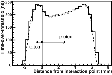
Figure 1: Time-over-threshold (TOT) for proton-triton tracks. This representative TOT distribution (solid line) was determined by averaging several thousand neutron events with a particular proton-triton track angle. The simulation result for the same track angle is overlaid (dashed line). Arrows indicate the direction of the proton and triton.

In the present paper, we introduce a more accurate method for finding the neutron position that not only produced a better spatial resolution but allowed us to include the entire range of track angles. Here, the neutron position was found by fitting the measured TOT distributions with the expected distributions (referred to as templates) determined using a simulation of our detector system. The simulation was based on the GEANT4 software toolkit [8] as described in Ref. [1]. The simulation result for a particular proton-triton track angle is shown in Fig. 1 (dashed line) along with the TOT distribution for real neutrons (solid line) at the same angle. The slight disagreement between the distributions is due to simplifications and uncertainties in the simulated response of the data acquisition hardware, coupled with the uncertainty in the neutron interaction position in the real data. The fitting, along with all data analysis for the results presented here, was carried out using custom software based on the ROOT object-oriented framework [9].

3 Spatial resolution

The spatial resolution was studied using images of cadmium test charts taken in March 2012 at NOBORU (NeutrOn Beamline for Observation and Research Use), located at Beamline 10 of the Materials and Life Science Experimental Facility (MLF) within the Japan Proton Accelerator Research Complex (J-PARC) [10]. The neutron pulse rate was 25 Hz (for a total neutron band-width at NOBORU of 10 Å) with a beam power of 200 kW, and a $3.2\times 3.2$ mm² collimator near the midpoint of the beamline provided a low-dispersion beam suitable for high-resolution imaging. The detector, located 15 m from the moderator, was filled with Ar-C₂H₆-³He (63:7:30) at 2 atm and equipped with a 2.5-cm drift cage as in Ref. [1], and the test charts were placed directly on the entrance window of the detector vessel. The detector was operated at a gas gain of 470, unless indicated otherwise.

Under these conditions, data was taken of one test chart for an exposure time of 7.8 minutes (not including data read-out time), and the resulting images, normalized to the beam profile, are shown in Fig. 2 for the various cuts described below. In the offline analysis, neutrons with energy well below the cadmium cut-off were selected by requiring a TOF greater than 2.1 ms ($270>E_{\rm neutron}>0.74$ meV, with the lower limit arising from the 10 Å bandwidth of NOBORU), and the gamma rejection cuts on total energy deposit and proton-triton track length described in our previous work were applied. Images were then reconstructed for three cut cases: 1) the above TOF and gamma cuts, 2) an additional consistency cut on the proton direction, and 3) the further requirement that the anode and cathode TOT distributions each displayed two distinct peaks (as in Fig. 1). The consistency cut required agreement in the component of the proton direction perpendicular to the plane of the $\mu$PIC (determined using the hit times) as measured independently by the anodes and cathodes. For cut case 1, the inconsistent events were corrected by changing the proton direction for the component with fewer hits, while they were simply removed in the second case. The last cut is the proton-triton separation (PTS) cut used in the method of Ref. [1]. The images of Figs. 2(a), 2(b), and 2(c) correspond to cut cases 1, 2, and 3, respectively. The image of Fig. 2(d), reconstructed using the simple method of Ref. [1] with the same cuts as 2(c), is shown for comparison. The number of events remaining after each cut are listed in Table 1, along with the event reconstruction efficiency, $\varepsilon_{rec}$, defined as the fraction of usable neutron events (i.e., those passing the TOF and gamma rejection cuts) included in the final images.

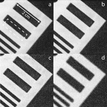
Figure 2: Images of a Cd test chart. Images reconstructed using the template method for (a) cut case 1, (b) cut case 2, and (c) cut case 3 as defined in the text. The image in (d) was reconstructed from the same data set using the simple algorithm of Ref. [1] and the same cuts as (c). Darker regions indicate higher neutron transmission. Bin size is 100 $\mu$m.

Table 1: Image reconstruction efficiency. Listed here are the number of events remaining after various selection cuts, along with the event reconstruction efficiency, $\varepsilon_{rec}$, for the imaging of a Cd test chart.

Cut	Number	Fraction	$\varepsilon_{rec}$ (%)	Figure
No cut	$4.20\times 10^{7}$	$-$
TOF $>2.1$ ms	$3.42\times 10^{7}$	1
Energy $>60$ clocks	$3.37\times 10^{7}$	0.986
Track length ($-2$/$+$3$\sigma$)	$2.77\times 10^{7}$	0.812	100	2(a)
Consistency cut	$1.83\times 10^{7}$	0.536	66.0	2(b)
PTS cut	$8.83\times 10^{6}$	0.258	31.8	2(c,d)

A detailed study of the spatial resolution was carried out using a 1.4-cm edge-section oriented at an angle of about 40^∘ relative to the anode strip direction (indicated in Fig. 2(a) by the dotted line). The resolution was studied using the modulation transfer function (MTF), calculated via Fourier transform from the discrete derivative of the intensity distribution across the edge, as in Ref. [11]. The observed edge spread function (ESF) and its derivative (line spread function, or LSF) are shown in Fig. 3(a) for cut case 1, with the resulting MTF shown in Fig. 3(b). (The distributions for the remaining cases were similar.) The MTF displays a clear Gaussian character and drops to 10% at around 2.5 lp/mm (line pairs/mm), or a line width of $\sim$200 $\mu$m. The Gaussian shape indicates that the correction for events with inconsistent proton direction is effective, since any significant contribution from events with incorrect proton direction would result in long tails in the ESF and LSF, producing a Lorentzian-like resolution function with an exponential MTF. From the shape of the ESF of Fig. 3(a) (or more specifically, its deviation from an error function), we estimate any remaining contamination from events with incorrect proton direction at less than 5%, with the effect on the measured resolution for cut case 1 smaller than our current error level. The values of the spatial resolution ($\sigma_{res}$) for Figs. 2(a), (b), and (c), determined by a Gaussian fit to the MTF, are listed in Table 2. Also listed are the resolutions determined from a second set of images with the chart rotated to orient the edge at roughly 0^∘ (i.e., nearly parallel to the anode strip direction), along with the weighted averages. The small differences in the results for the two edges are due mainly to their different positioning relative to the $\mu$PIC and beam center. The spatial resolutions for images reconstructed using the previous method [as in Fig. 2(d)] are also listed, and were found to be in good agreement with the result of our previous paper ($349\pm 43$ $\mu$m [1]).

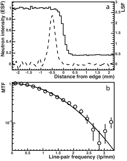
Figure 3: The modulation transfer function. Plot (a) shows the ESF (solid line) and LSF (dashed line) for the slit edge indicated in Fig. 2(a). The LSF has been shifted by $-0.5$ mm for ease of viewing. Bin size is 80 $\mu$m. Plot (b) shows the modulation transfer function (MTF) overlaid with the best-fit Gaussian.

Table 2: Spatial resolution from a Cd chart. Spatial resolutions ($\sigma_{res}$) for the three different cut conditions described in the text, as determined using edges oriented at 40^∘ and 0^∘ relative to the horizontal. Also listed are the resolutions for the same images reconstructed using the simple method of Ref. [1]. All values are given in $\mu$m.

Cut	$\sigma_{res}$
	40∘ edge	0∘ edge	Average
Tracking	$130.7\pm 3.1$	$136.5\pm 2.8$	$133.9\pm 2.1$
Consistency	$125.0\pm 3.3$	$131.5\pm 3.1$	$128.5\pm 2.3$
PTS	$111.2\pm 4.0$	$114.4\pm 3.7$	$112.9\pm 2.7$
Old method	$325\pm 19$	$343\pm 18$	$334\pm 13$

The improvement in the resolution observed between the three cut cases can be understood as the result of the dependence of the spatial resolution and proton direction determination on the proton-triton track angle, each worsening as the angle of the track approaches the perpendicular to the plane of the $\mu$PIC. Such tracks will have a smaller two-dimensional projection (i.e., the charge will be deposited in fewer strips), resulting in poorer fit results due to fewer data points and increasing ambiguity of the proton direction due to overlap of the proton and triton Bragg peaks. The consistency cut (cut case 2) thus tends to remove these ambiguous, low-information tracks, resulting in improved spatial resolution. Cut case 3 restricts the angles further by preferring tracks that are more parallel to the $\mu$PIC and distributed around 45^∘ relative to the anode and cathode strip directions, essentially maximizing the quality of the tracks and achieving the best spatial resolution.

3.1 Uniformity of the spatial resolution

To study the uniformity of the spatial resolution, an image of a regular slit pattern, shown in Fig. 4, was taken under the experimental conditions described previously with an effective exposure of 9.4 minutes. The slit pattern consisted of 0.5-mm wide slits cut into a 0.5-mm thick Cd plate at a pitch of 5 mm, and the chart was positioned with slits oriented along the anode strip direction. The resolution at each slit was determined by fitting the function:

$$N(x)=\frac{1}{2}A\left[{\rm erf}\left(\frac{x-(\mu-a)}{\sqrt{2}\sigma}\right)-{\rm erf}\left(\frac{x-(\mu+a)}{\sqrt{2}\sigma}\right)\right]+C$$ (1)

derived from the convolution of a Gaussian resolution with two step functions representing the slit. In the above fit function, $A$ is a normalization factor, erf is the usual Gaussian error function, $\mu$ and $a$ are the mean position and half-width of the slit, respectively, $\sigma$ is the Gaussian resolution, and $C$ accounts for the transmission of the Cd chart.

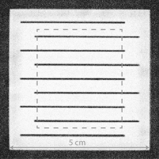
Figure 4: Image of slit pattern. A 0.5-mm thick Cd test chart with a pattern of 0.5-mm wide slits was used to study the uniformity of the spatial resolution. The gray dashed line indicates the area used for the study. Darker areas indicate higher neutron transmission. Bin size is 100 $\mu$m.

Fig. 5(a) shows a fit to one slit using the above equation, and Fig. 5(b) shows the spatial resolution found from seven such slits (circles) covering an area of roughly $3\times 3$ cm² near the beam center. The resolution determined from the slits is in good agreement with that determined previously from the edges using the MTF method, indicated in Fig. 5(b) by the filled square (40^∘ edge) and open square (0^∘ edge). The weighted average of all measurements yields a spatial resolution of $108.24\pm 0.74$ $\mu$m with a root-mean-square deviation (RMSD) of 6.4%, indicated as a percent of the spatial resolution.

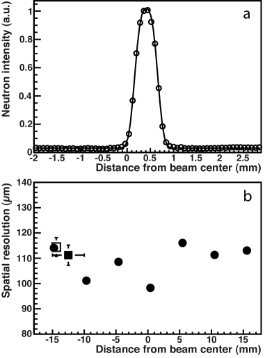
Figure 5: Uniformity of spatial resolution from slit pattern. Figure (a) shows the fit to the intensity distribution of a single 0.5-mm slit. Figure (b) shows the spatial resolutions determined for seven slits spaced at 5-mm intervals (circles), along with the resolutions determined via the MTF from the 40^∘ (filled square) and 0^∘ (open square) edges.

The observed non-uniformity in the spatial resolution, represented by the RMSD, arises from a combination of effects including parallax, variations in the $\mu$PIC gain and channel-by-channel amplifier responses, the underlying strip structure, and statistical fluctuations. As described in Ref. [1], parallax results from beam divergence coupled with the gas depth of the detector. Using our GEANT4 simulation with the beam geometry included, the worsening of the resolution due to the parallax effect was estimated at 2% near the beam center, increasing to 8% near $\pm$1.5 cm. Correcting the measured resolutions based on the simulation results gives a spatial resolution of $103.48\pm 0.77$ $\mu$m with an improved RMSD of 5.3%. Our GEANT4 simulation also indicates that the variations in the $\mu$PIC gain and channel-by-channel amplifier responses contribute about 15% to the remaining non-uniformity. Eliminating these variations, however, also results in a corresponding improvement in the spatial resolution such that the RMSD, as a fraction of the spatial resolution, remains roughly constant. Finally, while some small improvement can be expected with increased statistics, the effect of the underlying strip structure is difficult to address directly.

3.2 Spatial resolution versus gain

To check the effect of the gas gain on the spatial resolution, images of the edge at 0^∘ were taken at two additional gain settings, one higher ($\sim$850) and one lower ($\sim$285) than that used above, while the thresholds that determine TOT were held constant. The images were reconstructed using templates optimized for each gain setting, and the resulting spatial resolutions, found using the MTF procedure, are plotted in Fig. 6 for each of the three cut conditions. The resolution shows a clear trend, improving by roughly 3 $\mu$m for each decrease in gain of 100. A similar trend was observed for images generated with our GEANT4 simulation and was seen to continue to lower gain settings. This improvement can be understood as a result of the non-linearity of the relationship between pulse height and TOT [11], tending toward saturation for larger pulse heights (i.e., higher gains) and thereby decreasing the prominence of the proton and triton peaks in the TOT distribution.

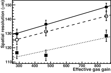
Figure 6: Spatial resolution versus gas gain. The results for the spatial resolution are plotted versus gas gain for three cut conditions: tracking cuts only (solid circles), with consistency cut (open circles), and with PTS cut (solid squares). Best fit lines are overlaid for each case.

This result indicates that a lower gas gain, or equivalently, that a smaller pulse-height-to-threshold ratio, is preferred for neutron imaging with our detector. The thresholds used for all measurements presented here (anodes: $-$2.5 mV, cathodes: $+$3.6 mV, with the difference arising from a larger intrinsic amplifier gain for positive pulses from the cathodes as discussed in Ref. [11]) were determined as the minimum needed to reject essentially all digital noise. While it may be possible to improve the spatial resolution at higher gain settings by increasing the discriminator thresholds, using the lowest possible gain (and thus, lowest thresholds) has two important advantages: 1) a low gain requirement increases the usable life of the gas for minimum ³He consumption, and 2) the electrical current generated on the $\mu$PIC is minimized, by minimizing the charge deposition per event, for stable high-rate operation. The lowest gain is limited by the neutron detection efficiency, which, while constant at higher gains, drops off rapidly below a gain of $\sim$200. This suggests a practical gain setting of around 250 for neutron imaging, safely within the region of constant efficiency. This would give an additional improvement of 5 to 6 $\mu$m in the spatial resolutions determined in the previous section. Incidentally, these optimized gain and threshold settings coincide with those shown in Ref. [1] to give a gamma sensitivity of $<$10^-12.

4 Discussion

The results of the previous section show that our $\mu$PIC-based detector can achieve a spatial resolution of just under 100 $\mu$m for the tightest cut condition (or $\sim$120 $\mu$m for all usable neutron events) after reducing the gas gain to the optimum value of 250 and correcting for beam divergence. This resolution compares well with that of imaging plates (25 to 50 $\mu$m) [12] and typical CCD detectors ($\sim$100$\mu$m) [13], with the advantages over these conventional imaging detectors of sub-$\mu$s time resolution and excellent gamma discrimination as discussed in Ref. [1]. The resolution of our detector also compares well with that of other imaging devices with TOF capability that have been or are being developed for use at pulsed neutron sources.

Table 3 shows a comparison of several such detectors, including the RPMT [14], consisting of a 0.25-mm thick ZnS(Ag)/⁶LiF scintillator coupled with a position sensitive photomultiplier tube, a stacked-GEM (gas electron multiplier) detector [15, 16] incorporating a cathode and GEMs coated with a thin boron film and an FPGA readout system, and a detector based on a boron-impregnated micro-channel plate (MCP) and Timepix readout chip [17, 18]. For the MCP, values for two operating modes are listed: a high-rate mode with spatial resolution dictated by the pixel size of the Timepix, and a high-resolution mode using the charge-centroid method to improve resolution at the cost of rate performance. The spatial resolution of our prototype exceeds that of both the RPMT and GEM detectors, while also exceeding the rate performance and efficiency of the RPMT. Our detector also has a much lower gamma sensitivity (by over three orders of magnitude) than the scintillator-based RPMT. No values are given for the gamma sensitivity of the remaining detectors, but they are also expected to outperform the RPMT. In particular, although the GEM-based detector should have gamma rejection similar to that of the $\mu$PIC, the detailed tracking with TOT information should give our $\mu$PIC detector the advantage. On the other hand, the stacked-GEM and MCP detectors show superior rate performance and detection efficiency. For the detection efficiency, however, that of our detector could be roughly doubled by adjusting the gas mixture to include more ³He, bringing it up to the level of the stacked-GEM and MCP detectors.

Table 3: Comparison of selected counting-type detectors with neutron time-of-flight capability. For the MCP detector, the values for an alternate high-resolution operating mode, when different from the normal mode, are given in parentheses.

Detector	Spatial	Time	Efficiency	Counting rate	Gamma	Typical	Ref.
	resolution	resolution	(at 25.3 meV)	(counts/s)	Sensitivity	area
$\mu$PIC	100–120 $\mu$m	0.6 $\mu$s	18%	200 kcpsa	$<10^{-12}$	$100$ cm2	[1]
RPMT	0.8 mm	10 $\mu$s	$\sim$6.5%b	$\sim$20 kcps	10-9	60 cm2	[14]
stacked-GEM	0.5 mm	$<0.1$ $\mu$sc	$\sim$25%b	12 Mcps	Not given	$100$ cm2	[15, 16]
MCP w/ Timepix	55 $\mu$m (15 $\mu$m)	$\sim$1 $\mu$s	$\sim$50%	$>0.5$ Gcps ($\sim$kcps)	Not given	$4$ cm2	[17, 18]

• Counting rate will increase to the order of Mcps after encoder upgrade [1].

• Estimated from quoted values (RPMT: 30%@0.95 nm, GEM: 30%@0.22 nm) using the appropriate neutron absorption cross-sections.

• Estimated from the electron drift velocity of Ar-CO₂ (70:30) gas and the given GEM spacing.

Future efforts to improve the spatial resolution of our detector will focus on optimization of the gas mixture and reduction of the gain variation and strip pitch of the $\mu$PIC. As discussed in Ref. [1], optimization of the gas mixture for reduced electron diffusion and/or shorter track lengths is expected to provide a 10 to 15% improvement in the spatial resolution, as determined by simulation. Also, as noted in Sec. 3.1, completely eliminating the gain variation would yield an improvement of around 15%. The gain variation may be reduced by improving the uniformity of the physical structures of the $\mu$PIC through tighter manufacturing controls. Furthermore, owing to the low operating gain, it becomes possible to reduce the size of the pixel structures in order to achieve a strip pitch as low as 200 $\mu$m, allowing us to take fuller advantage of the optimized gas properties. Using our GEANT4 simulation, we estimate that the spatial resolution would be reduced by $\sim$45% (or to less than 60 $\mu$m) after making all of the above improvements/modifications to the detector, hence achieving a spatial resolution similar to the MCP (in high-rate mode) and imaging plates.

Additionally, the rate performance of our detector will be significantly improved through a planned upgrade of the encoder hardware. As shown in Ref. [1], our current data acquisition system can handle raw data rates of $\sim$320 Mb/s (transferred to VME memory via a 32-bit parallel bus at 10 MHz), corresponding to a neutron count rate of roughly 200 kcps (kilo counts per second) for present detector conditions. Preliminary testing of the new encoder system indicates an increase of roughly a factor of four, resulting in a data rate of 12.8 Gb/s (or a neutron rate of 800 kcps). For a given data transfer rate, we can further increase the neutron count rate by reducing the amount of data per event in two ways: 1) by increasing the stopping power of the gas for shorter proton-triton track lengths, and 2) by performing some simple data processing on the FPGA. For instance, by replacing Argon with Xenon to reduce track lengths from 8 to 5 mm and calculating TOT on the FPGA, the amount of data per neutron event would be reduced by a factor of 3.2, achieving a neutron rate of over 2.5 Mcps. To approach the rate performance of the GEM-based detector, we could further reduce the track length to less than 2 mm by increasing the gas pressure above 5 atm, resulting in another factor of 3 or 4 increase in the neutron rate. Unfortunately, this last step would also reduce the spatial resolution (to the order of the 0.4 mm strip pitch), through a combination of increased scattering in the entrance window due to increased vessel thickness, increased electron diffusion, and the fact that we could no longer perform detailed tracking with so few hits per event. Such improvements to the spatial resolution and rate performance will be the subject of future studies.

5 Example: Resonance selective imaging

Neutron resonance absorption techniques take advantage of the tendency of some nuclides to preferentially absorb neutrons at specific energies, unique to each nuclide, to study isotopic composition and temperature [5]. Resonance absorption can be directly observed by measuring the neutron transmission spectrum of the sample, calculated as:

$$Tr({\rm TOF})=\frac{I({\rm TOF})}{I_{0}({\rm TOF})}$$ (2)

where $I({\rm TOF})$ and $I_{0}({\rm TOF})$ are the intensities measured with and without the sample, respectively. Due to the preferential absorption, the transmission will show sharp drops near a resonance. Such resonances typically occur for neutron energies above 1 eV and should appear in the TOF region between 0 and 1 ms for the 15-m flight path used in our experiment. The strength (depth) of the resonance dip gives the isotopic density, while thermal broadening allows us to deduce the temperature within the sample. The spatial distribution of the density and/or temperature can then be determined by measuring the transmission point-by-point. Using a 2-dimensional detector such as ours, this kind of measurement is greatly simplified.

As an example, we considered an image of a wristwatch taken in February 2011 at NOBORU, under conditions similar to those described in Sec. 3. Transmission spectra, calculated via Eq. 2, are shown in Fig. 7 for the main body of the watch (black line) and the watch battery only (gray line). The large resonance dip visible in the transmission of the watch battery around 0.46 ms (or a neutron energy of $E_{n}=5.2$ eV) is due to silver present in the battery’s cathode (along with many smaller dips at shorter TOFs). A dip due to copper is also visible around 45 $\mu$s (or 580 eV) in the main-body spectrum.

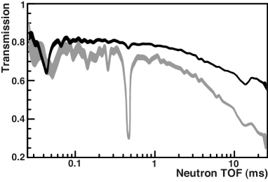
Figure 7: Neutron transmission spectra of a wristwatch. The transmission versus TOF is plotted for the main body (black line) and battery (gray line) of a wristwatch. The thickness of the lines indicates $\pm 1\sigma$ statistical error. Resonances due to copper and silver are visible around 0.04 and 0.46 ms, respectively. A Bragg edge is also visible around 15 ms.

Figs. 8(a) and 8(b) show radiographic images for neutrons with TOF $>2.1$ ms and $0.41<{\rm TOF}<0.51$ ms, respectively. (The gamma rejection cuts described in Sec. 3 are applied in both cases.) The TOF range of 8(b) selects neutrons with energy near the larger silver resonance, and although statistics are greatly reduced (necessitating a larger bin size for the image), the battery is clearly enhanced relative to the rest of the watch. A quantitative study of the determination of nuclide density via resonance absorption with a $\mu$PIC-based neutron imaging detector can be found in Ref. [19].

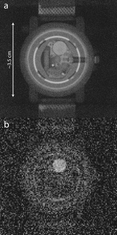
Figure 8: Images of a wristwatch taken at NOBORU, J-PARC. Radiographic images of a wristwatch are shown for neutron TOF ranges of (a) ${\rm TOF}>2.1$ ms and (b) $0.41<{\rm TOF}<0.51$ ms (darker areas correspond to higher neutron transmission). The TOF range for (b) corresponds to a resonance in the absorption cross-section of silver at a neutron energy of 5.2 eV. Bin sizes are (a) 80 $\mu$m and (b) 320 $\mu$m. Light, horizontal bands at the top and bottom of (a) are due to the aluminum-backed tape used to hold the watch in place.

Finally, note that a Bragg edge is visible in the spectra of Fig. 7 as a jump in the transmission around 15 ms. Such Bragg edges appear at the point where the neutron wavelength exceeds the Bragg-scattering condition for a particular set of crystal planes, and are observed for energies down to a few meV (or for a TOF up to about 20 ms in the present case). The Bragg edge observed here is most likely due to the metal body of the watch. From the position of the Bragg edge, one can determine the crystal spacing, and by studying the shape of the spectrum in the vicinity of the edge, one can learn about crystal properties such as grain size and texture [6]. Thus, in a single pulsed-beam measurement using a single detector, it is possible to study both the isotopic composition and crystal structure of a sample in two dimensions.

6 Conclusion

We have introduced a neutron position reconstruction method based on template fitting that improved both the spatial resolution and event reconstruction efficiency of our $\mu$PIC-based, time-resolved neutron imaging detector. The spatial resolution achieved with this method was found to be approximately Gaussian with a sigma of $108.24\pm 0.74$ $\mu$m and a non-uniformity of 6.4% RMSD (reconstruction efficiency $\varepsilon_{rec}=31.8$%). This represents a factor of three improvement over the resolution determined using the simple algorithm of our previous work [1]. By using less restrictive cut conditions, the reconstruction efficiency was greatly improved, while worsening the spatial resolution by only 14% (consistency cut, $\varepsilon_{rec}=66$%) and 19% (TOF and gamma cuts only, $\varepsilon_{rec}=100$%). Additionally, after reducing the gain to the optimum value of 250 and correcting for beam divergence, the spatial resolution of the $\mu$PIC would improve to just under 100 $\mu$m for the tightest cut condition (or $\sim$120 $\mu$m for TOF and gamma cuts only). The optimum gain setting of 250 also corresponds to that shown in Ref. [1] to give an effective gamma sensitivity of 10^-12 or less. Future improvements in the spatial resolution, to better than 60 $\mu$m, may be possible through optimization of the gas mixture for reduced electron diffusion, reduction of the gain variation of the $\mu$PIC through improved manufacturing controls, and reduction of the strip pitch.

We also demonstrated in the example measurement of Sec. 5 that by combining high-resolution imaging with event-by-event TOF measurement, our detector becomes a powerful and flexible tool for radiographic studies at pulsed neutron sources. Using such a detector, we can simultaneously record the radiographic image, resonance absorption, and Bragg-edge transmission information point-by-point, allowing a variety of material properties, including nuclide composition and density, internal temperature, crystal spacing, grain size and texture, internal strain, etc., to be studied in a single measurement. By utilizing computed tomography techniques, such measurements can also be extended to three dimensions, allowing non-destructive study of various bulk properties.

References

- [1] J.D. Parker et al., Nucl. Instr. and Meth. A 697 (2013) 23.
- [2] A. Ochi et al., Nucl. Instr. and Meth. A 471 (2001) 264.
- [3] R. Orito et al., IEEE Trans. Nucl. Sci., 51 (2004) 1337.
- [4] H. Kubo et al., in: IEEE Nuclear Science Symposium Conference Record (©2005 IEEE), 2005, p. 371.
- [5] H. Sato, T. Kamiyama, and Y. Kiyanagi, Nucl. Instr. and Meth. A 605 (2009) 36.
- [6] H. Sato, O. Takada, K. Iwase, T. Kamiyama, and Y. Kiyanagi, J. of Phys. Conf. Series 251 (2010) 012070.
- [7] J.R. Santisteban, L. Edwards, M.E. Fizpatrick, A. Steuwer, and P.J. Withers, Appl. Phys. A 74[Suppl.] (2002), S1433.
- [8] S. Agostinelli et al., Nucl. Instr. and Meth. A 506 (2003) 250; J. Allison et al., IEEE Trans. Nucl. Sci., 53 (2006) 270.
- [9] R. Brun and F. Rademakers, Nucl. Instr. and Meth. A 389 (1997) 81. See also http://root.cern.ch/.
- [10] F. Maekawa et al., Nucl. Instr. and Meth. A 600 (2009) 335.
- [11] K. Hattori et al., Nucl. Instr. and Meth. A 674 (2012) 1.
- [12] H. Kobayashi and M. Satoh, Nucl. Instr. and Meth. A 424 (1999) 1.
- [13] E.H. Lehmann, G. Frei, G. Kühne, and P. Boillet, Nucl. Instr. and Meth. A 576 (2007) 389.
- [14] K. Hirota et al., Phys. Chem. Chem. Phys. 7 (2005) 1836.
- [15] S. Uno et al., Phys. Proc. 26 (2012) 142.
- [16] S. Uno, T. Uchida, M. Sekimoto, T. Murakami, K. Miyama, M. Shoji, E. Nakano, and T. Koike, Phys. Proc. 37 (2012) 600.
- [17] A.S. Tremsin, J.B. McPhate, J.V. Vallerga, O.H.W. Siegmund, J.S. Hull, W.B. Feller, and E. Lehmann, Nucl. Instr. and Meth. A 604 (2009) 140.
- [18] A.S. Tremsin, J.B. McPhate, J.V. Vallerga, O.H.W. Siegmund, W.B. Feller, E. Lehmann, and M. Dawson, Nucl. Instr. and Meth. A 628 (2011) 415.
- [19] M. Harada, J.D. Parker, T. Sawano, H. Kubo, T. Tanimori, T. Shinohara, F. Maekawa, and K. Sakai, submitted to Physics Procedia.