‡
Invariant characterization of the growing and decaying density modes in LTB dust models.
Abstract
We obtain covariant expressions that generalize the growing and decaying density modes of linear perturbation theory of dust sources by means of the exact density perturbation from the formalism of quasi–local scalars associated to weighted proper volume averages in LTB dust models. The relation between these density modes and theoretical properties of generic LTB models is thoroughly studied by looking at the evolution of the models through a dynamical system whose phase space is parametrized by variables directly related to the modes themselves. The conditions for absence of shell crossings and sign conditions on the modes become interrelated fluid flow preserved constraints that define sub–cases of LTB models as phase space invariant subspaces. In the general case (both density modes being nonzero) the evolution of phase space trajectories exhibits the expected dominance of the decaying/growing in the early/late evolution times defined by past/future attractors characterized by asymptotic density inhomogeneity. In particular, the growing mode is also dominant for collapsing layers that terminate in a future attractor associated with a “Big Crunch” singularity, which is qualitatively different from the past attractor marking the “Big Bang”. Suppression of the decaying mode modifies the early time evolution, with phase space trajectories emerging from an Einstein–de Sitter past attractor associated with homogeneous conditions. Suppression of the growing mode modifies the late time evolution as phase space trajectories terminate in future attractors associated with homogeneous states. General results are obtained relating the signs of the density modes and the type of asymptotic density profile (clump or void). A critical review is given of previous attempts in the literature to define these density modes for LTB models.
pacs:
98.80.-k, 04.20.-q, 95.36.+x, 95.35.+d1 Introduction.
The spherically symmetric Lemaître–Tolman–Bondi (LTB) dust models [1] are a valuable tool to examine non–linear non–perturbative relativistic effects of cosmological and astrophysical self–gravitating systems by means of mathematically tractable methods (see the comprehensive reviews in [2, 3, 4, 5, 6]). They have been used as toy models in a wide variety of contexts: structure formation and late time cosmological inhomogeneities [7, 8], “void models” fitting cosmological observations without resorting to dark energy (see reviews in [4, 9]), testing averaging formalisms [10, 11, 12, 13, 14], cosmic censorship [15, 16] and even in quantum gravity [17].
The standard original set of metric variables is still used in most applications, as can be seen in the various book reviews [2, 3, 4], though void models often use different forms of “FLRW lookalike” variables that generalize FLRW observable parameters. Other alternative variables are the “quasi–local” (or “q–scalars”), associated with the weighted proper volume average of covariant scalars on comoving domains [18, 19], and successfully used in previous literature to undertake various theoretical issues: a dynamical systems approach to the models [20, 21], the asymptotic behavior of covariant scalars in the radial direction [22], the evolution of radial profiles and void formation [23], back–reaction and “effective” acceleration in the context of Buchert’s formalism [12, 13, 14] and even to study dark energy sources compatible with the LTB metric [24, 25]. As shown in [18, 19], the “FLRW lookalike” variables in void models are q–scalars, and the latter together with their associated fluctuations and perturbations are coordinate independent objects related to curvature and kinematic scalars, providing as well a complete representation of the dynamics of the models as “exact perturbations” on an FLRW abstract background defined by the q–scalars themselves (which satisfy FLRW time evolution laws).
An essential feature in linear perturbation theory of dust sources is the identification of decaying and growing density modes that are, respectively, dynamically dominant in the early and late stages of the evolution. An exact non–linear generalization of these perturbation modes were first obtained for LTB models by Silk [26] and re–derived by Krasinski and Plebanski [3]. However, these authors merely identified special initial conditions that define the “amplitudes” of the modes (and allow to “switch” them on or off), without carrying on any further analysis. More recently, Wainwright and Andrews [27] obtained expressions for the density modes by attempting to express a metric function as the sum of these modes along the lines of the “Goode-Wainwright” variables of Szekeres models. However, their key results are misleading because these authors did not consider fully general LTB models. A critical review of all this literature is given in Appendix A.
In the present article we extend and enhance all previous work described and summarized in the previous two paragraphs by taking advantage of the fact that the q–scalar perturbations define a self–consistent covariant perturbation formalism [19] that is analogous (and fully equivalent, as far as LTB models are concerned) to the 1+3 perturbation formalism of Ellis, Bruni, Dunsby and van Elst [28, 29, 30, 31, 32, 33]. Therefore, instead of the metric ansatz used in [27], the density growing and decaying modes are obtained from the q–scalar exact density perturbation, which has a clear covariant meaning in terms of the invariant ratio of Weyl to Ricci scalar scalar curvatures [18]. The resulting expressions for the modes are exact, fully analytic and coordinate independent, and their “amplitudes” are quantities conserved by the fluid flow. These expressions are also far less complicated and easier to handle than the expressions based on the fractional comoving density gradient that were used in previous work [3, 26, 27]. As a consequence, the density modes are useful to achieve a deeper understanding of various important theoretical features of the models, such as analytic solutions, simultaneity of the big bang singularity, regularity conditions for absence of shell crossings and radial profiles of the density and other covariant scalars. The effects of these modes in the dynamics of the models is best examined through a suitable dynamical system approach that unravels the connection between early/late time asymptotic inhomogeneous states and the dominance of the decaying/growing mode. This dynamical system also allows us to examine the dynamical effects of the suppression of either mode, showing that suppression of the decaying (or growing) mode leads to an invariant subspace characterized by asymptotic early (or late) time homogeneous states.
The section by section content of the article is given as follows. We provide in sections 2 and 3 the basic necessary background material: the description of LTB models in terms of q–scalars and their perturbations defined in an initial value parametrization of the metric and the analytic solutions expressed as constraints linking the proper time length along comoving worldlines (a q–scalar in itself) and any two basic q–scalars. By considering the exact analytic form of the density perturbation, we obtain in section 4 exact coordinate independent expressions for the density growing and decaying modes, which are shown in section 5 to reduce to the familiar expressions of linear perturbations theory in the linear limit. We introduce in section 6 a dynamical system such that the evolution of the models follows as trajectories in a 3–dimensional phase space parametrized by bounded variables directly related to the modes themselves. We analyze in sections 7 and 8 the phase space evolution of hyperbolic and elliptic models in the general case when both modes are nonzero, while the cases when the decaying or growing modes are suppressed are examined in sections 9 and 10. In sections 11 and 12 we examine the connection between the inhomogeneity of the models (as deviation from FLRW conditions) and the phase space evolution of the perturbations and invariant curvature and kinematic scalars associated with them. Appendix A provides a critical review of previous literature on the density modes [3, 26, 27] and in Appendix B we provide the forms of the metric and basic dynamical variables in terms of the standard original variables of the models.
2 LTB models, q–scalars and their perturbations.
We shall describe LTB dust models in the following useful FLRW–like metric parametrization
| (1) | |||
| (2) |
where satisfies the Friedman equation (8), is defined further ahead (see equation (7)) and the subindex 0 will denote henceforth evaluation at an arbitrary fiducial hypersurface . We remark that . The relation between this metric parametrization and the standard metric form and variables of the models is summarized in Appendix B.
It is useful to describe the dynamics of the models by means of their covariant objects given in terms of the representation of “q–scalars” and their perturbations (see [18, 19] for a comprehensive discussion). For every LTB scalar , the associated q–scalar and perturbation are defined by the correspondence rules 111We assume in the integrals in (3) that marks a symmetry center such that are nonzero and bounded and holds for all . We also exclude LTB models whose constant hypersurfaces have two symmetry centers (spherical topology) or no symmetry centers (“wormhole” topologies). However, these integrals can also be defined for such models (see [12, 23]). The q–scalars are related to proper volume averages with weight factor . See [18] for a comprehensive discussion.
| (3) | |||
| (4) |
where the second and third expressions in the right hand side of (4), which follow directly by differentiation and integration by parts of (3), allow us to computate in terms of the gradients and the scale factor .
The basic LTB covariant scalars are: (i) the rest–mass density , (ii) the Hubble scalar (with ) and (iii) the spatial curvature scalar (with the Ricci scalar of surfaces const.). In the q–scalar representation these scalars take the forms of exact perturbations [18, 19]
| (5) |
with their associated q–scalars and perturbations given by:
| (6) | |||
| (7) | |||
| (8) |
where the q–scalar is defined as
| (9) |
and the perturbations satisfy the following scaling laws:
| (10) | |||
| (11) |
Considering that (8), (9) and (11) provide algebraic constraints linking any two q–scalars and any two of their perturbations, it is evident that any LTB model can be uniquely specified by selecting as free parameters any two of the following four initial value functions: (notice that initial perturbations can always be obtained from (4) evaluated at ) 222The bang time , which is often taken as another initial value parameter, is expressible in terms of any two of these primary functions, see equation (21) in the following section.. As shown in [19], the models become fully determined in terms of any two q–scalars and their perturbations, which give rise to a covariant and gauge invariant formalism of exact spherical perturbations 333The perturbations are distinct from the standard metric induced “gauge invariant” perturbations [34] and from the covariant perturbations based on the 1+3 formalism [28, 29, 30, 31, 32, 33]. Their relation with simple “contrast” perturbations “” with respect to an FLRW background value [35] is discussed in detail in [19]..
The main proper tensors of the models, the shear tensor () and the electric Weyl tensor ( with the Weyl tensor), are expressible in terms of their eigenvalues and through a common symmetric trace–free tensor , with [30]:
| (12) | |||
| (13) |
where is also the only nonzero conformal invariant in a Newman–Penrose tetrad representation.
3 Analytic solutions as constraints among q–scalars.
In order to obtain fully determined analytic forms for the q–scalars and the perturbations as functions of time we need the solutions of the Friedman equation (8), which take the implicit form:
| (14) |
where is the Big Bang time such that for all . Notice that is a function of two q–scalars, hence it is itself a q–scalar [36] having an invariant meaning (from the fact that ): it is the total proper time (or affine parameter) length of the worldllines of comoving dust layers.
The functional forms of are given explicitly below (notice that these expressions yield as a function of by substitution of from the scaling laws (8) and (9)): 444We consider henceforth only hyperbolic and elliptic models or regions, thus we assume that and hold for all . The parabolic case follows as the limit or and is discussed in section 10.
| (15) | |||
| (18) |
with and given by
| (19) | |||
| (20) |
where arccosh correspond to the hyperbolic case and arccos to the elliptic case.
Substitution of in (15) and the expanding stage of (18) yields the Big Bang time and its gradient in terms of initial value functions and perturbations:
| (21) | |||
| (22) |
with
| (23a) | |||
| (23b) | |||
For hyperbolic models we have , but for elliptic models is restricted by , with:
| (23xa) | |||
| (23xb) | |||
where and mark the times of maximal expansion () and the collapse singularity (“Big Crunch” ).
4 Growing and decaying density modes.
Since the density perturbation generalizes dust density perturbations in the linear regime, it is worthwhile verifying if it can be decomposed in terms of growing and decaying modes. For this purpose, we use the exact solutions (15) and (18) to rewrite in (10) as
| (23xy) | |||
| (23xz) |
in which we identify:
| (23xaa) | |||
| (23xab) |
with the coefficients or “amplitudes” of the modes, and (both assumed nonzero unless stated otherwise) given in terms of primary initial value functions as
| (23xac) |
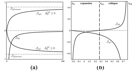
with and given by (22) and (23a). The scalars and , together with the restrictions on and from the conditions to avoid shell crossings (see sections 7–8), determine the time evolution of and that is displayed in figure 1. We provide in Appendix A a review and comparison with exact expressions obtained for these modes in previous literature [3, 27, 26], while Appendix B illustrates how these expressions can be computed in the traditional variables.
4.1 Properties of the density modes.
4.1.1 The modes amplitudes are fluid conserved quantities.
It is straightforward to prove by means of (10)–(11) and (22)–(23b) that the amplitudes and in (23xac) are fluid conserved quantities:
| (23xad) |
which follows from in (10) and the scaling laws
| (23xae) |
where and are the general forms for arbitrary of and given by (22) and (23a). The fluid conservation of their amplitudes allows us to write the growing and decaying modes as constraints between q-scalars and perturbations whose forms are also preserved by the fluid flow:
| (23xaf) |
with the conserved amplitudes and given by (23xad).
4.1.2 The density modes are coordinate independent quantities.
This follows from the fact that and are constructed with and (total proper time length along integral curves of the 4–velocity), while the amplitudes and are fluid conserved quantities given by (23xad).
4.1.3 The growing mode and spatial curvature.
The sign of the dimensionless covariant q–scalar in the growing mode in (23xaa) is closely related to the sign of the q–scalar associated to the spatial curvature (or , see (9)): 555Notice that is not the spatial curvature defined in (5). While the sign of determines the sign of , the converse is false: examples of elliptic LTB models (for which holds everywhere) exist in which holds in some domains (see [12]).
| (23xag) |
and thus provides a relation between and the type of kinematic evolution of dust layers as determined by the spatial curvature through or . Since these q–scalars are the analogues of the spatial curvature in FLRW models, the sign relation (23xag) provides an exact covariant generalization to the relation between the growing mode and the deviation from spatial flatness in linear perturbations around an Einstein–de Sitter background (see Appendix of [32]). We comment on this issue in the following section.
4.1.4 The remaining perturbations.
Considering the scaling laws (10)–(11) and the form of and in (23xy)–(23xz), we can express the remaining perturbations in terms of the growing/decaying modes :
| (23xaha) | |||||
| (23xahb) | |||||
| (23xahc) | |||||
where the following forms of and are useful for the purpose of computations:
| (23xahaia) | |||
| (23xahaib) | |||
| (23xahaiaj) |
where is given by (20) and we have assumed that . Notice that both and above can also be expressed in terms of the scale factor by means of the scaling laws (8) and (9).
5 Linear limit.
The exact form (23xy) illustrates the expected non–linear dependence of the density perturbation on the coupled modes and , as is not a linear perturbation, but an exact perturbation. In fact, is a solution of the non–linear evolution equation [19]
| (23xahaiak) |
However, under linear conditions characterized by and we recover well know results of the linear theory. A series expansion of (23xy) around and up to leading terms yields as a linear combination of the growing and decaying mode:
| (23xahaial) |
with given by (23xaa) and (23xab), which is the expected result of linear theory in which the growth of is directly controlled by the interplay between the completely decoupled modes , and thus it justifies the non–linear exact form (23xy) in which both modes are necessarily coupled. Notice that in the linear regime (23xahaial) the density perturbation diverges as if (because in (23xab)), while it remains finite in the non–linear regime (23xy) (see (23xahaianapatauavaxbabibkbnbobpbqbrbta) further ahead).
In the linear regime we have and , and thus (23xahaial) is the solution of the following equation for furnished by the linear limit of (23xahaiak):
| (23xahaiam) |
which is the known evolution equation for linear dust perturbations in the comoving gauge [19, 34, 35] once we consider that and are close to their FLRW values and .
The particular case of (23xahaiam) for a spatially flat FLRW background illustrates in a striking manner the direct relation between the density modes and the growth of 666The growth of the “density contrast” is often computed with the simple construction , where is the local density of an inhomogeneous model and is the density of a suitable FLRW background. As shown in [19], these simple “contrast perturbations” follow as the asymptotic limit as of non–local perturbations defined for LTB models that converge asymptotically to a FLRW state in the radial direction [22]. While and the “contrast perturbation” are different objects, they approximate each other in the linear limit. See [19] for a comprehensive discussion. . Expanding the solutions (15)–(18), as well as and given by (23xaa) and (23xab), around (or ) yields
| (23xahaiana) | |||
| (23xahaianb) | |||
| (23xahaianc) | |||
where we used (23xahaia) and (23xahaiaj), and then (9) to express the terms containing in terms of . It is worthwhile comparing these expansions with those obtained by Zibin [32] in looking at linear perturbations on an Einstein de Sitter background in the context of LTB models. From its form in (23xahaial) and considering (23xahaiana)–(23xahaianc), the linear limit of becomes formally identical to Zibin’s equation (A1) in Appendix of [32], which is the familiar expression of the linear dust density perturbation found in the literature (see also [35]). The expansion of in (23xahaiana), which coincides with Zibin’s equation (A3) in [32], illustrates the relation between the growing mode and the small deviations from spatial flatness (i.e. what Zibin in [32] calls the spatial curvature “fluctuations”) of linear perturbations around an an Einstein–de Sitter background in which is expected to be very small. This relation between and is described by Zibin as showing that “the curvature perturbation consists of just the growing mode”. However, this statement is not consistent with the quasi–local perturbation formalism described in [19]. The linear limits of the remaining exact perturbations in (23xaha)–(23xahc):
| (23xahaianao) |
show that the spatial curvature perturbation also depends on the decaying mode in its linar limit. Rather, in the framework of this formalism, the relation between and in (23xahaiana) is simply the perturbative version (around ) of the exact relation (23xag) connecting the growing mode and spatial curvature. Since spatial flatness () yields exactly , linear dust perturbations around an Einstein–de Sitter background will necessarily yield a perturbative form of the growing mode (23xaa) that is defined by small deviations from spatial flatness, but this does not imply that the spatial curvature perturbation is only defined by the growing mode. Notice that (23xag) also holds in the linear limit where and , taking the form , with its sign following the same relation with the curvature of FLRW time slices as (23xag) does with the quasi–local curvature of LTB time slices.
| 3-dimensional regions | ||
| Name | Description | Phase Space constraints |
| HYP | Hyperbolic models | |
| of the general case | ||
| complying with | ||
| Hellaby-Lake conditions. | . | |
| ELL | Elliptic models | |
| of the general case | ||
| complying with | ||
| Hellaby-Lake conditions. | ||
| (). | ||
| (). | ||
| 2–dimensional planes | ||
| Name | Description | Phase Space constraints |
| SDW | Suppressed Decaying Mode | |
| (simultaneous big bang). | . | |
| SGW | Suppressed Growing Mode | |
| elliptic & hyperbolic. | . | |
| VAC | Minkowski vacuum in | |
| non–standard coordinates. | ||
| Lines and points. | ||
| Name | Description | Phase Space constraints |
| PAR | Parabolic Models | |
| subset of SGM. | . | |
| FLRW | FLRW dust models | . |
| & center worldline. | ||
| EDS | Einstein De Sitter Model | . |
| subset of FLRW. | ||
| MINK | Minkowski | . |
| subset of VAC. | ||
6 The growing/decaying modes vs phase space invariant subspaces.
A phase space description is the ideal tool to examine the role of the growing and decaying modes in the dynamics of the models (see [20, 21] for previous work on dynamical systems applied to LTB models). For this purpose, it is convenient to construct a dynamical system whose phase space is parametrized by the following bounded variables directly related to and as defined in (23xaf): 777These variables are ill defined if there is a shell crossing singularity in which occurs at (or equivalently ).
| (23xahaianapa) | |||
| (23xahaianapb) | |||
where we used (23xae), with and given in terms of primary perturbations by the generalization for of (22) and (23a), while takes the form:
| (23xahaianapas) |
in which we considered all possible forms of in (23xahaia)–(23xahaib) with defined by (20).
The scaling laws for the q–scalars and their perturbations that have been previously derived [see (6)–(11), (23xy), (23xz), (23xaha)–(23xahc)] are analytic solutions of the evolution equations for the models, such as the following ones in the representation [19]:
| (23xahaianapata) | |||||
| (23xahaianapatb) | |||||
| (23xahaianapatc) | |||||
| (23xahaianapatd) | |||||
in which the expanding () and collapsing () stages of elliptic models must be treated separately, since and diverge as .
By eliminating and in terms of and from (23a)–(22) and (23xahaianapa)–(23xahaianapb):
| (23xahaianapataua) | |||
| (23xahaianapataub) | |||
and then substituting in (23xahaianapata)–(23xahaianapatd) we obtain the following self consistent dynamical system that is valid for all LTB models:
| (23xahaianapatauava) | |||||
| (23xahaianapatauavb) | |||||
| (23xahaianapatauavc) | |||||
where is defined by (23xahaianapas) and respectively correspond to (hyperbolic & elliptic expanding) and (elliptic collapsing), and the evolution parameter follows from applying the coordinate transformation [20, 21]
| (23xahaianapatauavaw) |
so that corresponds to that defines the initial slice (though the rest of the surfaces constant do not coincide with constant surfaces for ).
The evolution of each dust layer ( constant) in any given LTB model becomes a trajectory in the 3–dimensional phase space associated with (23xahaianapatauava)–(23xahaianapatauavc), determined by initial conditions specified at
| (23xahaianapatauavaxa) | |||
| (23xahaianapatauavaxb) | |||
where we used the fact that at to evaluate the initial values in (23xahaianapa)–(23xahaianapb) and with given by (23xahaianapas). Evidently, the phase space evolution of each LTB model determines a unique surface of generated by the trajectories once we consider the full range of in the initial conditions (23xahaianapatauavaxa)–(23xahaianapatauavaxb).
While the dynamical system (23xahaianapatauava)–(23xahaianapatauavc) can be solved numerically, its analytic solutions for any set of initial conditions (23xahaianapatauavaxa)–(23xahaianapatauavaxb) are readily available from the expressions previously derived for the phase space variables: is given the scaling law (9) expressed in terms of in (23xahaianapatauavaw):
| (23xahaianapatauavaxay) |
which substituted into (23xahaianapa)–(23xahaianapb) yields and as explicit functions of after using (20) to express in terms of given above.
The invariant subspaces of the phase space are constraints among the phase space variables that are preserved by the fluid flow (i.e. hold throughout the full time evolution). We remark that all constraints among the q–scalars and the perturbations can always be expressed as constraints among the phase space variables by elimination of by means of (10)–(11), (22), (23a), (23xy), (23xaha)–(23xahc) and (23xahaianapa)–(23xahaianapb). The invariant subspaces of relevant to the dynamics of the models provide a useful classification of subclasses of models and are listed and classified in Table 1, which also provides the conditions for absence of shell crossings given in terms of the phase space coordinates. In the following sections we examine qualitatively the phase space dynamics of the models, dealing first with the general case in which and are both nonzero, and then with the cases when each one of the density modes is suppressed.
| Critical Points. General case: . | ||
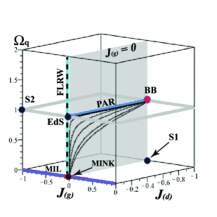
| Hyperbolic models. Section 7. Figure 2. | ||
| Symbol | Phase Space coordinates | Description |
| BB | Non–simultaneous Big Bang. | |
| Past attractor (source) | ||
| MIL | Milne. Future attractors (sinks) | |
| EdS | Einstein–de Sitter. Saddle | |
| S1 | Saddle | |
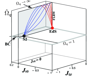
| S2 | Saddle | |
| Elliptic models. Section 8. Figure 3. | ||
| Symbol | Phase Space coordinates | Description |
| BB | Non–simultaneous Big Bang. | |
| Past attractor (source) | ||
| BC | Big Crunch. | |
| Future attractors (sinks) | ||
| EdS | Einstein–de Sitter. Saddle | |
| S2 | Saddle | |
7 The general case: hyperbolic models.
7.1 Absence of shell crossings.
Phase space trajectories are confined to the invariant subspace . However, avoidance of shell crossing singularities ( holds for all and all ) implies further restrictions on the region of containing the trajectories, as initial conditions must comply with the following constraints (the Hellaby–Lake (HL) conditions) [8, 22, 23]:
| (23xahaianapatauavaxaz) |
whose fulfillment implies the following fluid flow preserved constraints:
| (23xahaianapatauavaxbaa) | |||
| (23xahaianapatauavaxbab) | |||
| (23xahaianapatauavaxbac) | |||
where we have taken into consideration that and hold, together with using (23xy), (23xaha), (23xahaianapa)–(23xahaianapb) and (23xahaianapataua)–(23xahaianapataub) to eliminate in terms of . Since each one of the HL constraints (23xahaianapatauavaxbaa)–(23xahaianapatauavaxbac) defines an invariant subspace of , the phase space trajectories of all regular hyperbolic models are necessarily confined to the invariant subspace HYP in Table 1, defined by the intersection of (23xahaianapatauavaxbaa)–(23xahaianapatauavaxbac) and .
7.2 Critical points.
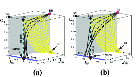
The critical points of the dynamical system (23xahaianapatauava)–(23xahaianapatauavc) () are listed in Table 2 and displayed by Figure 2. These points are located in the invariant subspace HYP. Notice that MIL is a subset of the invariant subspace VAC of Table 1 and BB corresponds to a non–simultaneous Big Bang ().
7.3 Asymptotic behavior.
All phase space trajectories evolve from the past attractor BB towards the future attractor MIL (see Table 2 and Figure 2), respectively corresponding to the early/late asymptotic limits and (equivalently and ). Considering (23xaa)–(23xab), (23xahaianapa)–(23xahaianapb) and (23xahaianapatauavaxay), the forms of in these asymptotic limits are given by:
-
•
Near BB: ():
(23xahaianapatauavaxbabba) (23xahaianapatauavaxbabbb) (23xahaianapatauavaxbabbc) -
•
Near MIL: ():
(23xahaianapatauavaxbabbbca) (23xahaianapatauavaxbabbbcb) (23xahaianapatauavaxbabbbcc)
where we have assumed in (23xahaianapatauavaxbabbc) that holds in order to fulfill (23xahaianapatauavaxbac). The following remarks are worth highlighting:
-
•
The limiting values of (23xahaianapatauavaxbabba)–(23xahaianapatauavaxbabbc) and (23xahaianapatauavaxbabbbca)–(23xahaianapatauavaxbabbbcc) fully coincide with the phase space coordinates of, respectively, BB and MIL given in Table 2.
-
•
The nonzero asymptotic late time limit of in (23xahaianapatauavaxbabbbcb) (line of sinks MIL in Table 2) depends the choice of initial conditions (i.e. ).
-
•
The asymptotic forms in (23xahaianapatauavaxbabba)–(23xahaianapatauavaxbabbc) and (23xahaianapatauavaxbabbbca)–(23xahaianapatauavaxbabbbcc) yield for whatever choice of initial conditions at :
(23xahaianapatauavaxbabd) which clearly illustrate the expected early times dominance of the decaying mode and late times dominance of the growing mode (see Figure 1a). Considering (23xaa), (23xac), (23xad) and (23xahaianapa), we have the following sign condition for each layer:
(23xahaianapatauavaxbabe) which defines the sign of and the common sign of and as invariant subspaces of for all trajectories with a given sign of .
-
•
As depicted by Figure 1a, we have at the past attractor BB and at the future attractor MIL, with remaining negative for all because of and (in compliance with (23xahaianapatauavaxaz)). On the other hand, goes from zero at BB to the finite terminal value (23xahaianapatauavaxbabbbcb) at the line of sinks MIL, with the sign of this terminal value determined by the sign of .
7.4 Phase space evolution.
Figure 2 displays typical phase space trajectories together with invariant subspaces and the critical points listed in Table 2. The curves were generated by the analytic expressions (23xahaianapa)–(23xahaianapb) and (23xahaianapatauavaxay) for initial conditions complying with the HL conditions (23xahaianapatauavaxaz), hence they are confined to the invariant subspace HYP bounded by the wireframe and solid surfaces (yellow and grey in the online version) defined by the HL constraints (23xahaianapatauavaxbaa)–(23xahaianapatauavaxbac) (see also Table 1). Following the asymptotic limits (23xahaianapatauavaxbabba)–(23xahaianapatauavaxbabbc) and (23xahaianapatauavaxbabbbca)–(23xahaianapatauavaxbabbbcc), the phase space coordinates are restricted for all trajectories to
| (23xahaianapatauavaxbabf) |
where we remark that must hold in compliance with (23xahaianapatauavaxaz). The curves evolve from the past attractor BB at (red circle), towards decreasing values of , avoiding the saddles EdS, S1, S2 (black circles) and the FLRW subspace (thick dotted vertical line). Each curve terminates in a point in the line of sinks MIL (subset of VAC) in the plane . The position of each sink as terminal point in MIL for each dust layer is given by the asymptotic value of (proportional to that of ), and is completely determined by initial conditions through the sign of (see section 7.4). As shown in section 11.4, the cases and respectively yield asymptotic void and clump density profiles at the future attractor MIL (see section 11.4). While initial conditions can be selected so that changes sign for different ranges of , the examples in Figure 2 have been selected so that (Figure 2a) and (Figure 2b) hold for all , with trajectories complying with (23xahaianapatauavaxbabe) for all . Hence, these trajectories evolve within invariant subspaces defined by the sign of .
8 The general case: elliptic models.
8.1 Absence of shell crossings.
Phase space trajectories are contained in the invariant subspace , but, as with regular hyperbolic models, the HL conditions to avoid shell crossings necessarily impose further restrictions on the region of where the trajectories are confined. The HL conditions for elliptic models are given by the following constraints among initial conditions [8, 22, 23]:
| (23xahaianapatauavaxbabg) |
The first two conditions above yield the same constraints as the first and third constraints in (23xahaianapatauavaxaz), while the joint fulfillment of the second and third condition above can be rephrased as the constraint:
| (23xahaianapatauavaxbabh) |
where we used the form for in (23xb) and from (23xahaianapatauavaxbabg). Notice that (23xahaianapatauavaxbabh) identifies as a necessary but not sufficient HL condition. Therefore, as a consequence of (19), (23xac), (23xae) and (23xad), the HL conditions (23xahaianapatauavaxbabg) and (23xahaianapatauavaxbabh) lead to the following constraints preserved by the fluid flow that must hold for the full evolution time range :
| (23xahaianapatauavaxbabia) | |||
| (23xahaianapatauavaxbabib) | |||
| (23xahaianapatauavaxbabic) | |||
| (23xahaianapatauavaxbabif) | |||
where is defined by (23xahaianapas) and we used the fact that holds for the full time evolution, as well as using (6)–(11), (19), (23xy), (23xaha), (23xahaianapa)–(23xahaianapb) and (23xahaianapataua)–(23xahaianapataub) to eliminate and in terms of . Notice that, as depicted by Figure 1b, the HL conditions imply that both density modes are negative in the expanding stage, while and in the collapsing stage.
As with hyperbolic models, each one of the HL constraints above is an invariant subspace of , hence, the invariant subspace of associated with regular elliptic models (denoted by ELL in Table 1) is the intersection of and each one of (23xahaianapatauavaxbabia)–(23xahaianapatauavaxbabif). All phase space trajectories of regular elliptic models are thus confined to ELL. The critical points are listed in listed in Table 2. Some of these points emerge in the dynamical system associated with the expanding stage and others from that of the collapsing stage.
8.2 Expanding stage.
The dynamical system is the same as that of hyperbolic models, but with and given by (20) with and arccos. The critical points (listed in Table 2) are: the past attractor BB and the saddles EdS and S2.
8.2.1 Asymptotic behavior.
-
•
Near the past attractor BB. The phase space variables have the same limiting values (23xahaianapatauavaxbabba)–(23xahaianapatauavaxbabbc) of hyperbolic models.
-
•
Near the maximal expansion. Late time evolution can be associated with the maximal expansion as (equivalently ). Phase space variables in this limit take the form:
(23xahaianapatauavaxbabibja) (23xahaianapatauavaxbabibjb) (23xahaianapatauavaxbabibjc) where and must hold because of the HL conditions (23xahaianapatauavaxbabg) and (23xahaianapatauavaxbabh).
8.3 Collapsing stage.
8.3.1 Critical points.
The appropriate dynamical system is (23xahaianapatauava)–(23xahaianapatauavc) with and given by (23xahaianapas) with . Its critical points (listed in Table 2) are the following: the EdS saddle and Big Crunch, the latter defining a line of future attractors associated with the collapsing singularity reached by dust layers as (or equivalently as ).
8.3.2 Behavior near the Big Crunch.
It is evident, from its phase space coordinates in Table 2, that the future attractor (the line of sinks BC) is radically different from the past attractor (source) BB of the expanding stage. This fact clearly indicates that the dynamics of dust layers near the collapsing singularity is qualitatively different from their behavior the initial big bang of the expanding stage.
Considering the appropriate forms of in (23xahaianapa) and (23xahaianapb) and the density modes in (23xaa) and (23xab), we have near the future attractor BC:
| (23xahaianapatauavaxbabibka) | |||
| (23xahaianapatauavaxbabibkb) | |||
where we took under consideration that and hold in compliance with (23xahaianapatauavaxbabic) and (23xahaianapatauavaxbabif). The following points are worth remarking:
-
•
The finite nonzero asymptotic forms of and in (23xahaianapatauavaxbabibka)–(23xahaianapatauavaxbabibkb) satisfy the constraint and provide the initial conditions dependent value of in Table 2. Since , these asymptotic forms are consistent with the known behavior as trajectories reach the Big Crunch BC (see [20, 21]).
-
•
The HL conditions (23xahaianapatauavaxbabic)–(23xahaianapatauavaxbabif) imply that (as in the expanding stage), but (see Figure 1b). While both and diverge near BC, the ratio of their magnitudes in (23xahaianapatauavaxbabibka)–(23xahaianapatauavaxbabibkb) together with the HL condition (23xahaianapatauavaxbabh) imply that the growing mode is dominant over the decaying mode in this limit:
(23xahaianapatauavaxbabibkbl) which re–affirms a late time behavior near BC that is qualitatively different from the early time behavior near the big bang in (23xahaianapatauavaxbabd).
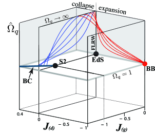
8.4 Phase space evolution.
The phase space trajectories of typical dust layers in the expanding and collapsing stage is depicted by Figure 3, where we use the variable (vertical axis) to associate the finite value to . Expanding and collapsing trajectories are respectively depicted in red and blue in the online version and critical points are listed in Table 2. The curves were obtained from the analytic expressions (23xahaianapa)–(23xahaianapb) and (23xahaianapatauavaxay), for initial conditions complying with the HL conditions (23xahaianapatauavaxbabg), hence they are confined to the invariant subspace ELL bounded by surfaces of defined by the HL constraints (23xahaianapatauavaxbabia)–(23xahaianapatauavaxbabif) (these surfaces are not displayed by figure 3). The curves evolve expanding from the Big Bang past attractor BB at (red circle), which is common to hyperbolic models, towards increasing values of , avoiding the saddles EdS, S2 (black circles) and the FLRW subspace. They reach maximal expansion as . In the collapsing stage they evolve towards decreasing , with each curve terminating in a point in the Big Crunch line of sinks BC (see Table 2) in the plane (dark blue thick line). The position of each sink as terminal point in BC for each dust layer is given by the asymptotic values of and given by (23xahaianapatauavaxbabibka) and (23xahaianapatauavaxbabibkb), and is completely determined by initial conditions.
9 Switching off the decaying mode.
| Critical Points. Suppressed Decaying Mode: . | ||
|---|---|---|
| Hyperbolic models. Section 9. Figure 4. | ||
| Symbol | Phase Space coordinates | Description |
| EdS | Einstein–de Sitter. Past attractor | |
| (source). Simultaneous Big Bang | ||
| MIL | Milne. Future attractors (sinks) | |
| S1 | Saddle | |
| Elliptic models. Section 9. Figure 5. | ||
| Symbol | Phase Space coordinates | Description |
| EdS | Einstein–de Sitter. Past attractor | |
| (source). Simultaneous Big Bang | ||
| S2 | Future attractor (sink), . | |
Suppression of the decaying mode yields hyperbolic and elliptic models 888Models with a suppressed decaying mode cannot be parabolic, since is inly compatible with (FLRW limit) if (see the following section). with initial conditions selected so that , which is equivalent to demanding (or equivalently ), which leads to a simultaneous big bang: constant. Initial conditions for these models follow from the analytic solutions (15)–(18):
| (23xahaianapatauavaxbabibkbm) |
where with given by (23xahaianapas), so that the remaining initial value functions can be obtained from (6)–(11) evaluated at . It is evident that these models can be fully determined by specifying a single free parameter, which can be in order to provide the easiest representation.
Models with a suppressed decaying mode evolve in the invariant subspace SDM in Table 1, which is the plane parametrized by with . However, the HL constrains (23xahaianapatauavaxbaa)–(23xahaianapatauavaxbab) and (23xahaianapatauavaxbabia)–(23xahaianapatauavaxbabic) further restrict the region of phase space evolution: if these constraints reduce to:
| (23xahaianapatauavaxbabibkbna) | |||
| (23xahaianapatauavaxbabibkbnb) | |||
and define invariant subspaces in the plane in which phase spaces trajectories are confined (we used the fact that for hyperbolic models).
The dynamical system (23xahaianapatauava)–(23xahaianapatauavc) also becomes reduced: the differential equation (23xahaianapatauavc) becomes a constraint that is identically satisfied, with the two remaining equations (23xahaianapatauava)–(23xahaianapatauavb) leading to the 2–dimensional dynamical system
| (23xahaianapatauavaxbabibkbnboa) | |||
| (23xahaianapatauavaxbabibkbnbob) | |||
whose critical points are listed in Table 3.
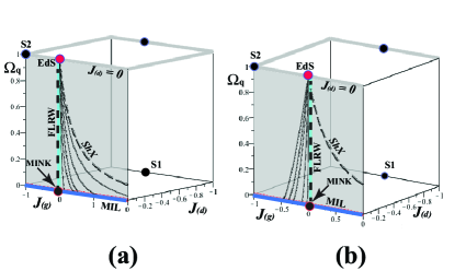
The phase space evolution is depicted by Figures 4 and 5. The trajectories are confined to the invariant subspace SDM. We have the following features:
-
•
Hyperbolic models (Figure 4). The early time evolution is radically different from that of the general case, as trajectories emerge from the EdS past attractor (red circle), but the late time evolution is qualitatively similar: curves evolve towards decreasing and terminate at the future attractor (line of sinks) MIL of the general case (dark blue thick line). The position of each curve in MIL depends on initial conditions given by the terminal value (23xahaianapatauavaxbabbbcb). Curves with (Figure 4a) or (Figure 4b) respectively terminate with positive or negative values of . As shown in section 11.4, initial conditions or respectively determine a void or clump density profile for the whole evolution.
-
•
Expanding stage of elliptic models (Figure 5). The curves are depicted in red in the online version. The early time evolution is qualitatively the same as that of hyperbolic models described above, but the curves evolve towards increasing to a late time regime given by the maximal expansion as analogous to the general case.
-
•
Collapsing stage of elliptic models. The curves are depicted in blue in the online version. They evolve from the maximal expansion towards the future attractor point S2, contained in the line of sinks BC of the general case. Again, the behavior near the collapse singularity is qualitatively different from that near the initial singularity in the expanding stage (past attractor EdS).
As we discuss in sections 11 and 12, the early time phase space behavior around the EdS past attractor is the characterization of the early time homogeneity associated with models with suppressed decaying mode.
10 Switching off the growing mode.
| Critical Points. Suppressed Growing Mode: . | ||
|---|---|---|
| Hyperbolic models: . Section 10. Figure 6. | ||
| Symbol | Phase Space coordinates | Description |
| BB | Non–simultaneous Big Bang. | |
| Past attractor (source) | ||
| MINK | Minkowski. Future attractor (sink) | |
| EdS | Einstein–de Sitter. Saddle | |
| S1 | Saddle | |
| Parabolic models: . Section 10. Figure 6. | ||
| Symbol | Phase Space coordinates | Description |
| BB | Non–simultaneous Big Bang. | |
| Past attractor (source) | ||
| EdS | Einstein–de Sitter. Future attractor (sink). | |
Models characterized by a suppressed growing mode follow from either one of the following combination of restrictions:
| (23xahaianapatauavaxbabibkbnbobpa) | |||
| (23xahaianapatauavaxbabibkbnbobpb) | |||
where is defined in (19) and we used . These restrictions lead to the following set of restricted initial conditions:
| (23xahaianapatauavaxbabibkbnbobpbqa) | |||
| (23xahaianapatauavaxbabibkbnbobpbqb) | |||
so that a single free parameter is sufficient to fully determine these models.
The phase space evolution is contained in the invariant subspace SGM in Table 1, which is the plane parametrized by , with the line corresponding to parabolic models (the invariant subspace PAR SGM in Table 1). The HL constraints (23xahaianapatauavaxbabia)–(23xahaianapatauavaxbabif) for elliptic models with cannot be fulfilled, hence all regular models with a suppressed growing mode must be either hyperbolic models with or parabolic models, both complying with (from the HL constraints (23xahaianapatauavaxbaa)–(23xahaianapatauavaxbac)).
For hyperbolic models complying with the dynamical system (23xahaianapatauava)–(23xahaianapatauavc) reduces to the 2–dimensional system
| (23xahaianapatauavaxbabibkbnbobpbqbra) | |||
| (23xahaianapatauavaxbabibkbnbobpbqbrb) | |||
whose critical points are listed in Table 4.
For parabolic models () the system (23xahaianapatauavaxbabibkbnbobpbqbra)–(23xahaianapatauavaxbabibkbnbobpbqbrb) further reduces to a single dynamical equation that determines the line PAR in Table 1:
| (23xahaianapatauavaxbabibkbnbobpbqbrbs) |
where is given by (23xahaianapatauavaxb). The two critical points of (23xahaianapatauavaxbabibkbnbobpbqbrbs) are listed in Table 4.
The phase space evolution of models with a suppressed growing mode is depicted by figure 6. A qualitative description is provided below:
-
•
Hyperbolic models. Because of the HL constraints, the phase space trajectories are contained in the restriction of SGW (see Table 1), and thus, they are qualitatively analogous to those of the general case for early times near the past attractor BB. However, the late time evolution is qualitatively different: all phase space trajectories terminate at the Minkowski sink MINK associated with an asymptotic homogeneous vacuum state as .
-
•
Parabolic models. They evolve in the invariant subspace PAR from the Big Bang past attractor BB ( ) to the future attractor EdS ( ). This future attractor singles out these models as the only LTB models whose asymptotic late time evolution is qualitatively analogous to that of an Einstein de Sitter model.
11 Phase space evolution of the perturbations.
Besides their coordinate independent nature [18], the define a self–consistent gauge invariant perturbation formalism on a FLRW background associated with the q–scalars (see [19] for a comprehensive discussion). Therefore, it is useful to examine the relation between the density modes and the phase space evolution of these perturbations (specially the density perturbation ).
11.1 Early times regime.
If the decaying mode is nonzero (), this mode completely dominates the early time behavior of the perturbations, since and hold near the past attractor BB associated with a non–simultaneous big bang (these remarks also hold when the growing mode is suppressed ). For whatever choice of initial conditions (23xahaianapatauavaxa)–(23xahaianapatauavaxb), we have from (23xy) and (23xaha)–(23xahb):
| (23xahaianapatauavaxbabibkbnbobpbqbrbta) | |||
| (23xahaianapatauavaxbabibkbnbobpbqbrbtb) | |||
| (23xahaianapatauavaxbabibkbnbobpbqbrbtc) | |||
| (23xahaianapatauavaxbabibkbnbobpbqbrbtd) | |||
which clearly illustrate how the dominance of the decaying mode is associated with a very inhomogeneous early times behavior of the scalars and since does not hold (the exception being ). This early time inhomogeneity can be appreciated by looking at the consequences of the limit in (23xahaianapatauavaxbabibkbnbobpbqbrbta): it indicates a very different behavior of the local density, , and its associated q–scalar, , in the early time regime:
| (23xahaianapatauavaxbabibkbnbobpbqbrbtbu) |
where we assumed that holds (in compliance with (23xahaianapatauavaxaz)) and used , as well as (23xy) and (23xahaianapatauavaxbabibkbnbobpbqbrbta). While both densities diverge near BB, they diverge at very different rates with , so that , which provides a measure of inhomogeneity because can be associated with the density of an abstract FLRW background (see [19]).
If the decaying mode is suppressed (), the past attractor is no longer BB but the EdS point associated with a simultaneous big bang (see figures 4 and 5). The early time behavior of the in the limit (or ) is radically different from the corresponding limits when in (23xahaianapatauavaxbabibkbnbobpbqbrbta)–(23xahaianapatauavaxbabibkbnbobpbqbrbtc):
| (23xahaianapatauavaxbabibkbnbobpbqbrbtbv) |
where for hyperbolic and elliptic models, is defined in (23b) and having the same limit as (i.e. (23xahaianapatauavaxbabibkbnbobpbqbrbtd)). Evidently, the elimination of the decaying mode suppresses the early time inhomogeneity in the density and Hubble factor, as they decay at the same FLRW rate as their associated q–scalars: and , though this does not occur for the spatial curvature (unless we demand the extra condition in (23xahaianapatauavaxbabibkbnbobpbqbrbtbv)).
11.2 Late times regime.
If the growing mode is nonzero ( and ), this mode completely dominates the late time behavior of the perturbations, since and hold, either near the future attractor MIL of hyperbolic models (), or the maximal expansion () in elliptic models (see figure 1). The behavior of the density perturbation in both cases follows directly from (23xy):
| (23xahaianapatauavaxbabibkbnbobpbqbrbtbwa) | |||
| (23xahaianapatauavaxbabibkbnbobpbqbrbtbwb) | |||
with the perturbation having the same late time limit as in (23xahaianapatauavaxbabibkbnbobpbqbrbtbwa) for hyperbolic models (from (23xahb)), while for elliptic models we have and as (an expected result since and hold in this limit). The remaining perturbations and vanish near MIL. Notice how the dominance of the growing mode yields an asymptotic nonzero value for and that is proportional to , which indicates the existence of an inhomogeneous late time density (the “residual inhomogeneity” reported in [27]).
11.3 The collapsing regime.
Near the future attractor BC (see Table 2), associated with the collapsing singularity (Big Crunch), the perturbations take the same asymptotic inhomogeneous forms (23xahaianapatauavaxbabibkbnbobpbqbrbta)–(23xahaianapatauavaxbabibkbnbobpbqbrbtd). However, the interpretation of these limits is radically different, as they are not associated with a dominant decaying mode, but a dominant growing mode. This follows from the fact that both modes and diverge in (23xahaianapatauavaxbabibka)–(23xahaianapatauavaxbabibkb) (see also Figure 1), with (from (23xahaianapatauavaxbabibkbl)), while and reach nonzero finite terminal values such that . Another important difference is the fact that the limits (23xahaianapatauavaxbabibkbnbobpbqbrbta)–(23xahaianapatauavaxbabibkbnbobpbqbrbtd) also hold for elliptic models with a suppressed decaying mode as trajectories approach the future attractor S2 (see Figure 5 and section 9), while near the Big Bang past these limits only hold when the decaying mode is nonzero (the past attractor BB). In a sense, the description of conditions near BC allows us to disentangle the behavior near BC from that near BB, given the fact that the perturbations reach the same limits near both critical points. Hence, regardless of the existence of a decaying mode, there is a clear inhomogeneous growing mode dominated behavior near the Big Crunch that is qualitatively analogous to that of the Big Bang with a nonzero dominating decaying mode.
11.4 Density radial profiles.
As shown in [23], the relation between the gradients and the density perturbation (see (4)) leads to a close connection between the sign of and the type of density radial profile: over density or “clump” if and under density or “void” if (for a comprehensive discussion see [23]). The close relation between the density radial profiles and the growing mode emerges from the fact (see lemmas 7 and 9 and Table 1 of [23]) that initial conditions that govern the evolution of these profiles depend on the sign of in (23a), which determines the sign of and (see (23xaa), (23xac), (23xahaianapa) and (23xad)). Therefore, considering the early and late time limits of in (23xahaianapatauavaxbabibkbnbobpbqbrbta), (23xahaianapatauavaxbabibkbnbobpbqbrbtbv) and (23xahaianapatauavaxbabibkbnbobpbqbrbtbwa)–(23xahaianapatauavaxbabibkbnbobpbqbrbtbwb), we arrive to the following general results relating density profiles and the sign of the density growing mode:
-
•
If the growing mode is positive () a density void profile necessarily emerges in the late time evolution. This applies only to those regular hyperbolic models with initial conditions , irrespective of whether the decaying mode is zero or not (Figures 2a and 4a).
-
•
If the growing mode is positive () and the decaying mode is zero () a density void profile occurs for the whole time evolution. This applies only to those regular hyperbolic models with initial conditions (Figure 4a).
-
•
If the growing mode is negative () a density clump profile necessarily occurs for the whole time evolution. This applies to all regular elliptic models (Figures 3 and 5) and to regular hyperbolic models with initial conditions , irrespectively of whether the decaying mode is zero or not (Figures 2b and 4b).
These general results involving the sign of the growing mode may seem to be counter–intuitive, because they are opposite to the “conventional wisdom” from the astrophysical literature [3, 4, 35], whereby a positive growing mode is associated with an increasing “density contrast” in the formation of an over–density (clump), while a negative growing mode becomes intuitively connected to a decreasing “density contrast” in the formation of an under–density or void (see especially examples in [3, 4, 7], see [19] for a comprehensive discussion on this issue).
The definition of “clump” or “void” profiles can be extended to other scalars [19, 23]. For regular hyperbolic models it is straightforward to show that the pattern of profile evolution of is qualitatively analogous to the profile evolution of and , while as shown in Table 1 of [23], the profile pattern of is approximately the opposite to that of and . The evolution of radial profiles of and exhibits a much weaker relation to the signs of the density models (see [23]).
12 Inhomogeneity in terms of invariant scalars.
The perturbations are covariant objects directly related to curvature and kinematic invariants [18]:
| (23xahaianapatauavaxbabibkbnbobpbqbrbtbwbx) |
| (23xahaianapatauavaxbabibkbnbobpbqbrbtbwbya) | |||
| (23xahaianapatauavaxbabibkbnbobpbqbrbtbwbyb) | |||
where is the Ricci scalar, the scalars are defined in (12) and (13) and we used the fact that . Evidently, and provide an invariant measure of the deviation from FLRW homogeneity through the ratio of Weyl to Ricci curvature () and anisotropic to isotropic expansion (). The remaining perturbations and can also be expressed in terms of these invariants by substituting (23xahaianapatauavaxbabibkbnbobpbqbrbtbwbya) and (23xahaianapatauavaxbabibkbnbobpbqbrbtbwbyb) into (10)–(11) or (23xaha)–(23xahb). We have the following possibilities on the relation between and the density modes:
-
•
If the decaying mode is not suppressed (), these ratios take the following early time forms near the past attractor BB
(23xahaianapatauavaxbabibkbnbobpbqbrbtbwbybz) where we assumed that holds in compliance with (23xahaianapatauavaxbabg).
-
•
If the decaying mode is suppressed (), then both ratios vanish near the past attractor EdS.
-
•
If the growing mode is not suppressed, the ratio takes the following forms in late time regime:
(23xahaianapatauavaxbabibkbnbobpbqbrbtbwbycaa) (23xahaianapatauavaxbabibkbnbobpbqbrbtbwbycab) with the ratio vanishing near MIL and diverging near maximal expansion (because and ).
-
•
If the growing mode is suppressed (), then both ratios take the same form as (23xahaianapatauavaxbabibkbnbobpbqbrbtbwbybz) near BB and both vanish in the future attractor MINK.
-
•
In the collapsing regime has the same form as in (23xahaianapatauavaxbabibkbnbobpbqbrbtbwbybz) near BC, but takes the form:
(23xahaianapatauavaxbabibkbnbobpbqbrbtbwbycacb) where we used (23xahaianapatauavaxbabh) and the form for in (23xb).
It is important to remark that in most cases above increases as the evolution proceeds and the growing mode becomes dominant, the exceptions to this rule are the following two cases with suppressed decaying mode: hyperbolic models with and elliptic models, since goes from at the past attractor EdS towards negative late time values (23xahaianapatauavaxbabibkbnbobpbqbrbtbwbycaa)–(23xahaianapatauavaxbabibkbnbobpbqbrbtbwbycab) (notice that is a necessary HL condition for elliptic models).
13 Summary and final discussion.
We have found analytic exact covariant expressions ( in (23xaa) and (23xab), section 4) that generalize for LTB dust models the density growing and decaying modes of linear perturbation theory of dust sources (section 5). To achieve this task we considered the exact density perturbation, , that emerges from the description of LTB dynamics furnished by the quasi–local (q–scalars) and their local perturbations , which were studied comprehensively in [18, 19] (the necessary background material appears in sections 2 and 3). As shown in these references, the q–scalars and their perturbations are themselves covariant scalars related to curvature and kinematic invariants (see section 12), and in particular the yield a rigorous self–consistent formalism of exact perturbations in which a “FLRW background” is defined by the . Since this formalism reproduces in the linear limit the results of linear perturbation theory (in the comoving gauge), we show in section 5 that the linear limit of the exact growing and decaying modes are consistent with their corresponding forms obtained in previous literature [32] for linear perturbations on an Einstein–de Sitter background.
The relation between and the dynamical behavior of LTB models was studied thoroughly by means of a dynamical system defined in section 6, whose associated 3–dimensional phase space is parametrized by the q–scalar (which generalizes the FLRW Omega factor) and two variables (see (23xahaianapa)–(23xahaianapb)) that are closely related to . Hence, dust layers are curves (phase space trajectories) evolving between the critical points in (listed in Tables 2, 3 and 4), with the full set of trajectories of each model defining a unique 2–dimensional surface in . This phase space study, which is applicable to any LTB model admitting at least one symmetry center, represents an important improvement over previous work using a dynamical systems approach to LTB models [20, 21], since: (i) we now describe the Hellaby–Lake (HL) regularity conditions (absence of shell crossing singularities) as fluid preserved constraints that are effectively invariant subspaces of , and (ii) we provide a full description of the expanding and collapsing regimes of elliptic models in a unified phase space. The phase space approach developed in this paper also represents a significant improvement over previous articles that used other means to obtain exact expressions for the density modes [3, 26, 27] (see Appendix A for a critical review of this literature).
Considering the HL conditions as fluid preserved constraints, the density modes provide an effective classification of regular LTB models in 4 non–vacuum subclasses that define regions of that are invariant subspaces, so that all phase space trajectories of any of these subclasses are entirely confined to its corresponding region. These 4 subclasses were examined separately: hyperbolic and elliptic models in the general case when both density modes are nonzero (subspaces HYP and ELL discussed in sections 7 and 8), and models in which one of the modes is suppressed: suppressed decaying mode (invariant subspace SDM, section 9) and suppressed growing mode (invariant subspace SGM, which contains parabolic models PAR, section 10). The main results of this phase space study are:
-
•
For all LTB models of the general case the early time evolution is governed by the decaying mode (), whereas in the late time evolution (even in the collapsing stage) the growing mode is dominant (). The signs of the modes are determined by the fulfillment of the HL conditions. The time evolution of and for a typical dust layer was displayed in Figure 1.
-
•
For all models in which the decaying mode is nonzero ( at early times from the HL conditions) the phase space trajectories begin their evolution in a past attractor BB (see sections 7, 8 and 10, as well as Figures 2, 3 and 6 and Tables 2 and 4), associated with a non–simultaneous Big Bang and very inhomogeneous early time conditions (see discussion in sections 11.1 and 12).
-
•
If the decaying mode is suppressed, the past attractor is the Einstein de Sitter point EdS, associated with a simultaneous Big Bang and early time homogeneous conditions (see sections 9, 11.1, Figures 4 and 5 and Table 3).
-
•
Phase space trajectories of hyperbolic models with nonzero growing mode (regardless of the value of the decaying mode) terminate in a line of sinks that define a future attractor MIL, associated with the Milne spacetime contained in the VAC invariant subspace of vacuum LTB models (see Tables 1, 2 and 4, and Figures 2 and 4). Since at MIL, there is a terminal density inhomogeneity proportional to the amplitude of the growing mode , with (see section 11.4) the terminal density profile being a void () or clump (). If the decaying mode is suppressed, we have the same pattern but this void/clump form of the density profile holds for the whole evolution (see section 11.4 and 12). If the growing mode is suppressed the future attractor is the Minkowski point MINK (contained in MIL), with and thus with homogeneous terminal density (see Figure 6 and Table 4).
-
•
Parabolic models are a subset of models with suppressed growing mode, evolving along the line PAR contained in the subspace SGM. They are described by a single trajectory that goes from the BB past attractor of the general case towards a future attractor given by the EdS point (see section 10, Figure 6 and Table 4). These are the only LTB models whose late time evolution approaches an Einstein de Sitter FLRW model.
-
•
The future attractor of trajectories of the collapsing stage of all elliptic models with nonzero decaying mode is the line of sinks BC, associated with the Big Crunch singularity (see Figure 3, Table 2 and section 8). If the decaying mode is zero, the future attractor is the point S2 contained in BC (see Figure 5, Table 3 and section 9). Hence, irrespective of the decaying mode, the dynamical behavior near the Big Crunch is dominated by the growing mode, and thus is qualitatively distinct from that near the Big Bang. This is an inherent feature of inhomogeneous models that is absent in FLRW re–collapsing models [21], even if the perturbations yield the same limiting values near both singularities (see section 11.3). However, the difference in behavior near these singularities becomes evident when examined in terms of the density modes and invariant scalars (see sections 11.3 and 12).
The invariant curvature and kinematic scalars, and , as defined by (23xahaianapatauavaxbabibkbnbobpbqbrbtbwbx) and (23xahaianapatauavaxbabibkbnbobpbqbrbtbwbya)–(23xahaianapatauavaxbabibkbnbobpbqbrbtbwbyb), convey important dynamical information when we highlight their close relation with the density modes. The asymptotic early time diverging form of the ratio of Weyl to Ricci curvature in (23xahaianapatauavaxbabibkbnbobpbqbrbtbwbybz) is consistent with the notions of a “non-isotropic” initial singularity and “primordial inhomogeneity”, normally associated with a dominant nonzero decaying mode, which radically changes to an “isotropic” initial singularity and “primordial homogeneity” when vanishes as this mode is suppressed. The late time forms (23xahaianapatauavaxbabibkbnbobpbqbrbtbwbycaa)–(23xahaianapatauavaxbabibkbnbobpbqbrbtbwbycab) are consistent with the notion of “residual density inhomogeneity” associated with a nonzero growing mode (see [27] for complementary discussion). However, notice that a nonzero decaying mode also introduces an early time primordial inhomogeneity in the Hubble scalar and spatial curvature , while a nonzero growing mode does not introduce “residual inhomogeneity” in and , since the late time vanishing of and implies that the invariant scalar also vanishes in this limit.
The role of the density modes can also be relevant in the use of LTB models to fit cosmological observations, in particular, the preference of models with a suppressed decaying mode in void models is justified [9] (see the dissenting view in [37]) on the grounds that these models exhibit an early time Einstein de Sitter homogeneity (the past attractor EdS in models with , see section 9 and Figures 4 and 5). However, the demand that the decaying mode must be strictly (mathematically) zero may be too stringent, as it yields initial conditions that are too restrictive and (strictly speaking) LTB models no longer provide an appropriate description of cosmological conditions for times before the last scattering surface, and thus compatibility with observations may be achieved as long as perturbations are sufficiently small at this surface even if is not strictly zero (see [38, 39, 40]). Looking at this issue is beyond the scope of this paper and will be pursued separately.
Finally, it is important to remark that the work we have undertaken in this paper can be generalized to LTB models with nonzero cosmological constant. For this purpose the analytic solutions derived in [41, 42] can be used to identify the density modes in the exact perturbation (see also [21]). Evidently, the case leads to a completely different late time dynamical behavior of the models, and this must be reflected in the exact forms of the density modes. Another necessary generalization is to non–spherical Szekeres models, proceeding along the lines of [36], and likely to even more general inhomogeneous spacetimes. These extensions of the present work are currently under elaboration and will be submitted for publication in the near future.
Appendix A Review of previous literature.
Exact expressions for the density growing and decaying mode were obtained first by Silk in [26], which were re–derived by Krasinski and Plebanski in section 18.19 of reference [3], and more recently by Wainwright and Andrews in [27].
Silk (and Krasinsky–Plebanski afterwards) considered density perturbations defined by the “comoving fractional density gradient” [28, 29, 31] in the traditional variables (see Appendix B), which (from (23xahaianapatauavaxbabibkbnbobpbqbrbtbwbych)) involves the explicit computation of
| (23xahaianapatauavaxbabibkbnbobpbqbrbtbwbycc) |
for hyperbolic and elliptic models, using the parametric solutions of the Friedman equation (8) to eliminate and in terms of and and their gradients. Since the resulting form of is too cumbersome, these authors only examined the asymptotic limits (hyperbolic and elliptic models) and (hyperbolic models) of various subexpressions in order to identify the initial conditions that suppress either one of the modes amplitudes ( and which directly relate to and ). Notice that the parameters of [3] respectively correspond to defined in (23a) and (23b). There is no attempt in [26] or [3] to obtain the full expressions of the modes or to study their relation with generic properties of the models (regularity conditions or density profiles). As a contrast, we have used the density perturbation in (10) and (23xy), related to the gradient by (4), which allows us to identify the same amplitudes and yields much more tractable subexpressions for the modes (just compare the elegance and simplicity of (23xaa) and (23xab) with the rather awkward equations of section 18.19 of [3]).
Wainwright and Andrews considered exactly the same metric (1)–(2) [their equation (2.1)], with satisfying the Friedman equation (8) [their equation (2.5)] with and their parameters respectively corresponding to . They used the ansatz , with the “deviation function” given in the Goode–Wainwright form , which (according to the authors) identifies the growing () and decaying () modes.
However, Wainwright and Andrews assumed without any justification that their parameter (i.e. ) is constant, which (in general) is not true, and thus their study removes unjustifiably an important degree of freedom in the set of initial conditions. As a consequence, the following key results are only valid for the rather uninteresting particular case of models admitting a constant initial density ():
-
•
The relation between and the ratio of quadratic invariant scalar contractions of the Weyl and Ricci tensors [their equation (2.8)] is not valid in general. If we consider the full degrees of freedom does not comply with such ratio, taking instead the form:
(23xahaianapatauavaxbabibkbnbobpbqbrbtbwbycd) where is the only nonzero conformal invariant in a Newman–Penrose representation and is the 4–dimensional Ricci scalar. Evidently, if we recover the equation (2.8) of Wainwright and Andrews, as the scalar contractions and are respectively proportional to and (see [18]).
-
•
The evolution equation for [their equation (2.9)] is in general given by:
(23xahaianapatauavaxbabibkbnbobpbqbrbtbwbyce) and reduces to (2.9) of Wainwright and Andrews only if (equivalent to ). As a consequence, the general evolution equation for is not given by (2.10).
-
•
Equation (3.5) is not general. Hence, following these authors, if we define the growing/decaying modes from in the general case we obtain
(23xahaianapatauavaxbabibkbnbobpbqbrbtbwbycf) which yields their equations (3.7) and (3.8) only if . However, while the forms for and in (3.7) and (3.8) do coincide with (22) and , and thus allow us to express the decaying mode (23xab) as the product , it is not possible (in general) to express the term as a product that would allow for the identification of the growing mode (23xaa) and its amplitude (23a).
Since the assumption “” carries along the rest of their paper, some (or a lot) of the results of Wainwright and Andrews may be misleading or even mistaken. In particular, a decomposition of the growing/decaying modes in terms of the Goode–Wainwright variables obtained form the metric function does not seem to be possible in general. In contrast, such decomposition leading to the correct linear limit is possible and consistent through the density perturbation in (23xy). Besides the issue of consistency, we remark that is not a metric function, but a coordinate independent quantity related by (23xahaianapatauavaxbabibkbnbobpbqbrbtbwbya) to the ratio of invariant scalars and .
Appendix B LTB models in their standard variables.
LTB models are usually described in their original variables by the metric and field equations:
| (23xahaianapatauavaxbabibkbnbobpbqbrbtbwbycg) | |||
| (23xahaianapatauavaxbabibkbnbobpbqbrbtbwbych) |
with the analytic solutions of the Friedman–like equation above usually given in parametric form (though these solutions can also be given in the implicit forms (15)–(18)).
We can obtain the metric (1) and the q–scalar variables from (23xahaianapatauavaxbabibkbnbobpbqbrbtbwbycg) and (23xahaianapatauavaxbabibkbnbobpbqbrbtbwbych) by selecting the radial coordinate so that and re–scalling as
| (23xahaianapatauavaxbabibkbnbobpbqbrbtbwbyci) | |||
| (23xahaianapatauavaxbabibkbnbobpbqbrbtbwbycj) |
with and given in terms of by
| (23xahaianapatauavaxbabibkbnbobpbqbrbtbwbyck) |
All the results of this article can be immediately re-written in terms of the variables by direct substitution of (23xahaianapatauavaxbabibkbnbobpbqbrbtbwbyci), (23xahaianapatauavaxbabibkbnbobpbqbrbtbwbycj) and (23xahaianapatauavaxbabibkbnbobpbqbrbtbwbyck) in the appropriate scaling laws and analytic expressions.
References
References
- [1] Lemaître G 1933 Ann. Soc. Sci. Brux. A 53 51. See reprint in Lemaître G 1997 Gen. Rel. Grav. 29 5; Tolman R C 1934 Proc. Natl Acad. Sci. 20 169; Bondi H 1947 Mon. Not. R. Astron. Soc. 107 410.
- [2] Krasiński A, Inhomogeneous Cosmological Models, Cambridge University Press, 1998.
- [3] Plebanski J and Krasinski A, An Introduction to General Relativity and Cosmology, Cambridge University Press, 2006.
- [4] K. Bolejko, A. Krasiński, C. Hellaby, M.-N. Célérier, Structures in the Universe by exact methods: formation, evolution, interactions, Cambridge University Press, Cambridge 2009
- [5] Celerièr M N 2007 New Advances in Physics 1 29 (Preprint arXiv:astro-ph/0702416)
- [6] Bolejko K Celerier M N and Krasinski A 2011 Class Quant Grav 28 164002 (Preprint arXiv:1102.1449v2 [astro-ph.CO])
- [7] Krasiński A and Hellaby C 2002 Phys Rev D 65 023501; Krasiński A and Hellaby C 2004 Phys Rev D 69 023502; Krasiński A and Hellaby C 2004 Phys Rev D 69 043502; Hellaby C and Krasiński A 2006 Phys Rev D 73 023518; Bolejko K Krasiński A and Hellaby C 2005 MNRAS 362 213 (Preprint arXiv:gr-qc/0411126); Bolejko K Krasinski A and Hellaby C 2005 Mon Not Roy Astron Soc 362 213-228 (Preprint arXiv:0411126v2[gr-qc])
- [8] Matravers D R and Humphreys N P 2001 Gen. Rel. Grav. 33 531 52; Humphreys N P, Maartens R and Matravers D R 1998 Regular spherical dust spacetimes (Preprint gr-qc/9804023v1)
- [9] Marra V and Notari A 2011 Class. Quant. Grav. 28 164004 (Preprint arXiv:1102.1015)
- [10] Chuang C H, Gu J A and Hwang W Y P 2005 Class.Quant.Grav.,25, 175001 Preprint astro-ph/0512651
- [11] Paranjape A and Singh T P 2006 Class.Quant.Grav.,23, 6955 6969
- [12] Sussman R A 2008 On spatial volume averaging in Lema tre–Tolman–Bondi dust models. Part I: back reaction, spacial curvature and binding energy (Preprint arXiv:0807.1145 [gr-qc])
- [13] Sussman R A 2010 AIP Conf Proc 1241 1146-1155 (Preprint arXiv:0912.4074 [gr-qc])
- [14] Sussman R A 2011 Back-reaction and effective acceleration in generic LTB dust models To appear in Class.Quant.Grav. (Preprint arXiv:1102.2663v1 [gr-qc])
- [15] Eardley D M 1974 Commun Math Phys 37 287; Eardley D M and Smarr L 1979 Phys Rev D 19 2239; Dyer C C 1979 MNRAS 189 189; Waugh B and Lake K 1988 Phys Rev D 38 1315; Waugh B and Lake K 1989 Phys Rev D 40 2137; Lemos J P S 1991 Phys Lett A 158 279
- [16] Joshi P S and Dwivedi I H 1993 Phys Rev D 47 5357; Joshi P S and Singh T P 1995 Phys Rev D 51 6778; Dwivedi I H and Joshi P S 1997 Class. Quant. Grav. 47 5357
- [17] Vaz C, Witten L and Singh T P 2001 Phys Rev D 63 104020; Kiefer C, Mueller-Hill, Vaz C 2006 Phys Rev D 73 044025; Bojowald M, Harada T and Tibrewala R 2008 Phys Rev D 78 064057
- [18] Sussman R A 2013 Class Quant Grav 30 065015 (Preprint arXiv:1209.1962v3 [gr-qc])
- [19] Sussman R A 2013 Class Quant Grav 30 065016 (Preprint arXiv:1301.0959v2 [gr-qc])
- [20] Sussman R A 2008 Class Quantum Grav. 25 015012 Preprint arXiv:gr qc/0709.1005
- [21] Sussman R A and Izquierdo G 2011 Class Quantum Grav. 28 045006 Preprint arXiv:gr qc/1004.0773
- [22] Sussman R A 2010 Gen Rel Grav 42 2813–2864 (Preprint arXiv:1002.0173 [gr-qc])
- [23] Sussman R A 2010 Class.Quant.Grav. 27 175001 (Preprint arXiv:1005.0717 [gr-qc])
- [24] Sussman R A Quasi-local variables and inhomogeneous cosmological sources with spherical symmetry 2008 AIP Conf.Proc. 1083 228-235 Preprint arXiv:0810.1120.
- [25] Sussman R A 2009 Phys Rev D 79 025009 (Preprint arXiv:arXiv:0801.3324 [gr-qc])
- [26] Silk J 1977 Astron and Astroph 59 53
- [27] Wainwright J and Andrews S 2009 Class.Quant.Grav.,26, 085017
- [28] Ellis G F R and Bruni M 1989 Phys Rev D 40 1804
- [29] Bruni M, Dunsby P K S and Ellis G F R 1992 Astroph. J. 395 34–53
- [30] van Elst H and Ellis G F R 1996 Class Quantum Grav 13 1099-1128 (Preprint arXiv:gr-qc/9510044)
- [31] Ellis G F R and van Elst H 1998 Cosmological Models (Cargèse Lectures 1998) Preprint arXiv gr-qc/9812046 v4
- [32] Zibin J P 2008 Phys Rev D78 043504 [arXiv:0804.1787]
- [33] Dunsby P et al 2010 JCAP 06 017 (Preprint arXiv:1002.2397v1 [astro-ph CO])
- [34] Bardeen J 1980 Phys Rev D 22 1882; Bardeen J, Steinhardt P and Turner M S 1983 Phys Rev D 28 679
- [35] Padmanabhan T 2002 Theoretical Astrophysics, Volume III: Galaxies and Cosmology (Cambridge University Press).
- [36] Sussman R A and Bolejko K 2012 Class Quantum Grav 29 065018 (Preprint arXiv:1109.1178)
- [37] Cèlèrier M N Bolejko K and Andrzej Krasiński A 2010 Astron Astrophys 518 A21 [arXiv:0906.0905v5]
- [38] Clarkson C and Regis M 2011 JCAP 02 013 (Preprint arXiv:1007.3443v2[astro-ph CO])
- [39] Zibin J P 2011 Phys Rev D84 123508 (Preprint arXiv:1108.3068)
- [40] Bull F Clifton T and Ferreira P G 2012 Phys Rev D85 024002 (Preprint arXiv:1108.2222)
- [41] Valkenburg W 2012 Gen Rel Grav 44 2449-2476 (Preprint arXiv:1104.1082)
- [42] Romano A E and P Chen 2011 JCAP 10 016 (Preprint arXiv:1104.0730)