Sparse Adaptive Dirichlet-Multinomial-like Processes
 

Abstract

Online estimation and modelling of i.i.d. data for short sequences over large or complex “alphabets” is a ubiquitous (sub)problem in machine learning, information theory, data compression, statistical language processing, and document analysis. The Dirichlet-Multinomial distribution (also called Polya urn scheme) and extensions thereof are widely applied for online i.i.d. estimation. Good a-priori choices for the parameters in this regime are difficult to obtain though. I derive an optimal adaptive choice for the main parameter via tight, data-dependent redundancy bounds for a related model. The 1-line recommendation is to set the ‘total mass’ = ‘precision’ = ‘concentration’ parameter to $m/[2\mskip 3.0mu\ln{n+1\over m}]$, where $n$ is the (past) sample size and $m$ the number of different symbols observed (so far). The resulting estimator (i) is simple, (ii) online, (iii) fast, (iv) performs well for all $m$, small, middle and large, (v) is independent of the base alphabet size, (vi) non-occurring symbols induce no redundancy, (vii) the constant sequence has constant redundancy, (viii) symbols that appear only finitely often have bounded/constant contribution to the redundancy, (ix) is competitive with (slow) Bayesian mixing over all sub-alphabets.

Contents

1. 1 Introduction
2. 2 Preliminaries
3. 3 The Main Model
4. 4 Redundancy of $S^{\beta}$ for General $\beta$
5. 5 Redundancy for Approximate Optimal $\beta^{*}$
6. 6 Redundancy for Variable ${\smash{\vec{\beta}^{*}\mskip-3.0mu}}$
7. 7 Comparison to Other Methods
8. 8 Conclusion
9. References
10. A Approximations of the (Di)Gamma Function
11. B Proof of Theorem 2
12. C Derivation of Approximate Optimal $\beta^{*}$
13. D Proof of Theorem 4
14. E Proof of Theorem 5
15. F Improvement on $\beta^{*}$
16. G Bayesian sub-alphabet weighting
17. H Algorithms & Applications & Computation Time
18. I Experiments
19. J List of Notation

Keywords

sparse coding; adaptive parameters; Dirichlet-Multinomial; Polya urn; data-dependent redundancy bound; small/large alphabet; data compression.

1 Introduction

The problem of estimating or modelling the probability distribution of data sequences sampled from an unknown source is central in machine learning [Bis06], information theory [CT06], and data compression [Mah12]. I consider the case where the data items are complex and/or are drawn from a large space. Many approaches to language modelling and document analysis [MS99] fall into this regime, where data items are words. Typical documents comprise a small fraction of the available 100’000+ English words, and words have different length/complexity/frequency.

Online estimation of i.i.d. data. More formally, I consider i.i.d. data with base alphabet ${\cal X}$ much larger than the sequence length, which implies that only a small fraction of symbols (which in case of text are words) appear in the sequence. I focus on online algorithms that at any time can predict the probability of the next symbol given only the past sequence and without knowing the actually used alphabet ${\cal A}$ and/or symbol occurrence frequencies in advance.

While real-word data like text are often not i.i.d, i.i.d. estimators are often a key component of more sophisticated models. For instance, in $n$-gram models, the subsequence of words that have the same length-$n$ context is (assumed) i.i.d. Since these subsequences can be very short, good i.i.d. estimators for short sequences and huge alphabet are even more important. The same holds for variable-order models like large-alphabet context tree weighting [TSW93], and in addition, the employed i.i.d. estimators need to be online.

Performance measures. Performance can be measured in many different ways: code length [CT06], perplexity [MS99], redundancy [Wal05], regret [Grü07], and others. The most wide-spread (across disciplines) performance measures are transformations of the (estimated) data likelihood(s). If $Q(x_{1:n})$ is the estimated probability of sequence $x_{1:n}\equiv x_{1}...x_{n}$, then $\log 1/Q(x_{1:n})$ is the optimal code length and $Q(x_{1:n})^{1/n}$ the perplexity of $x_{1:n}$. If $P$ is some reference measure, then $\log 1/Q-\log 1/P$ is the redundancy of $Q$ relative to $P$. For log-loss, this is also its regret, though many variations are used. Many other performance measures can be upper bounded by (expected) code length [Hut03]. I therefore concentrate on $-$log-likelihood = code length and redundancy.

Dirichlet-multinomial and parameter choice. The Dirichlet-multinomial distribution is defined as $\text{DirM}(x_{n+1}=i|x_{1:n})={n_{i}+\alpha_{i}\over n+\alpha_{+}}$, which can be motivated in many ways, e.g. by the Polya urn scheme or as below. This process and extensions thereof like the Pitman-Yor process are widely studied and applied [BH10], in particular for language processing and document analysis. Theoretically motivated choices for the Dirichlet parameters $\alpha_{i}$ are $\alpha_{i}={{}^{1}\mskip-3.0mu/\mskip-3.0mu_{2}}$ for the Krichevsky-Trofimov (KT) estimator [KT81] and Jeffreys/Bernardo/MDL/MML prior [Jef46, Jef61, Ber79, Grü07, Wal05], $\alpha_{i}=0$ for Frequentist and Haldane’s prior [Hal48], $\alpha_{i}=1$ for the uniform/indifference/Bayes/Laplace prior [Bay63, Lap12], and $\alpha_{i}=1/|{\cal X}|$ for Perks’ prior [Per47].They are all problematic for large base alphabet ${\cal X}$, so is sometimes optimized or sampled experimentally or averaged with a hyper-prior. The following table summarizes these choices:

$$\begin{array}[]{c||c|c|c|c||c}\text{Dirichlet}&\text{Laplace}&\text{KT\&others}&\text{Perks}&\text{Haldane}&\text{Hutter}\\ \hline\cr\alpha_{i}=\displaystyle{\alpha_{+}\over|{\cal X}|}\rule{0.0pt}{17.22217pt}&1&\displaystyle{1\over 2}&\displaystyle{1\over|{\cal X}|}&0&\displaystyle{m\over 2|{\cal X}|\ln{n+1\over m}}\end{array}$$ (1)

The last column is a glimpse of the results in this paper, where $m$ is the number of different symbols that appear in $x_{1:n}$. For continuous spaces ${\cal X}$, the Dirichlet process is usually parameterized by a base distribution $H()$ and a critical concentration parameter $\beta\widehat{=}\alpha_{+}$.

Main contribution. In this paper I introduce an estimator $S$ [Eq.(2)], which essentially estimates the probability of the next symbol by its past relative frequency, but reserves a small (or large!) “escape” probability to new symbols that have not appeared so far. Such escape mechanisms are well-known and used in data compression such as prediction by partial match (PPM) [CW84, Mah12]. This is (somewhat) different from how the Dirichlet-multinomial regularizes zero frequency with $\alpha_{i}>0$ or $\beta>0$.

The main contribution is to derive an “optimal” escape parameter $\beta^{*}$ [Eq.(16) offline and Eq.(21) online]. The key to improve upon existing estimators like the minimax optimal KT estimator is to consider data-dependent redundancy bounds, rather than expected or worst-case redundancy, and find its minimizing $\beta$. While the KT estimator and many of its companions have ${\textstyle{1\over 2}}\log n$ redundancy per symbol in ${\cal X}$, whether the symbol occurs in the sequence or not, our new estimator $S^{\beta^{*}}$ suffers zero redundancy for non-occurring symbols, and essentially only ${\textstyle{1\over 2}}\log n_{i}+O(1)$ for symbols $i$ appearing $n_{i}$ times. This is never much worse and often significantly better than KT. This also leads to an “optimal” variable Dirichlet parameter ${\smash{\vec{\beta}^{*}\mskip-3.0mu}}$. While knowing ${\smash{\vec{\beta}^{*}\mskip-3.0mu}}$ is practically useful, the derived redundancy bounds themselves are of theoretical interest.

Contents. After establishing notation in Section 2, I motivate and state my primary model $S^{\beta}$ in Section 3. I derive exact expressions and upper and lower bounds for the redundancy of $S^{\beta}$ for general constant $\beta$ in Section 4, and show how they improve upon the minimax redundancy. I approximately minimize the redundancy w.r.t. $\beta$ in Section 5. There are various regimes for the optimal $\beta^{*}$ and the used alphabet size $|{\cal A}|$, even with negative redundancy. To convert this into an online model, I make $\beta^{*}$ time-dependent in Section 6, causing very little extra redundancy. In Section 7 I theoretically compare my models to the Dirichlet-multinomial distribution, and Bayesian sub-alphabet weighting. Section 8 concludes.

Proofs of the lower and two upper bounds can be found in Appendices B, D, and E, a derivation of $\beta^{*}$ in Appendix C with improvements in Appendix F, details of Bayesian subset-alphabet weighting in Appendix G, algorithmic considerations in Appendix H, and an experimental evaluation in Appendix I. Used properties of the (di)Gamma functions can be found in Appendix A, and a list of used notation in Appendix J.

2 Preliminaries

All global notation is introduced in this section and summarized in Appendix J.

Base alphabet (${\cal X}$, $D$). Let ${\cal X}$ be the base alphabet of size $D=|{\cal X}|$ from which a sequence of symbols is drawn. If not otherwise mentioned, I assume ${\cal X}$ to be finite. I have a large base alphabet in mind, but this is not a technical requirement. The alphabet could literally consist of e.g. ASCII symbols, could be the set of (over 100’000) English words, or just bits $\{0,1\}$. Indeed, even finiteness of ${\cal X}$ is nowhere crucially used and all results generalize easily to countable and even continuous ${\cal X}$ as we will see.

Total sequence ($n$, $x_{1:n}$, $n_{i}$). I consider sequences $x_{1:n}\equiv(x_{1},...,x_{n})\in{\cal X}^{n}$ of length $n$ drawn from ${\cal X}$. Let $n_{i}$ be the number of times, $i$ appears in $x_{1:n}$. I have in mind that the sequences are sampled independent and identically distributed (i.i.d), but I actually never use this assumption. All results in this paper hold for any individual fixed sequence $x_{1:n}$, and only depend on the order statistics $\boldsymbol{n}=(n_{i})_{i\in{\cal X}}$. The crucial parameters are $n$, $D$, the number $m$ of non-zero counts, and model parameter $\beta$ introduced later, which induces several different regimes, second by the counts $n_{i}$.

Used alphabet ($m$, ${\cal A}$, $i,j,k$, $\nu$, $\bar{\nu}$). Only a subset of symbols ${\cal A}:=\{x_{1},...,x_{n}\}\subseteq{\cal X}$ may actually appear in a sequence $x_{1:n}$. Our model is primarily motivated for the regime where the number $m=|{\cal A}|$ of used symbols is much smaller than $D=|{\cal X}|$, as e.g. any English text uses only a small fraction of all possible words. It turns out that our model can be tuned to actually perform very well for all possible $1\leq m\leq\min\{n,D\}$: constant sequences ($m=1$), every symbol appearing only once ($m=n$), and all available symbols appear ($m=D$). Indices $i,j,k$ are understood to range respectively over symbols in ${\cal X}$, ${\cal A}$, and ${\cal X}\setminus{\cal A}$. Without loss of generality I can assume $i\in{\cal X}=\{1,...,D\}$, $j\in{\cal A}=\{1,...,m\}$, and $k\in{\cal X}\setminus{\cal A}=\{m+1,...,n\}$. I also use $\bar{\nu}:=n/m$ for the average multiplicity of symbols in $x_{1:n}$, and $\nu:=m/n$ is its inverse.

Current sequence and observed alphabet ($t$, $x_{1:t}$, ${\cal A}_{t}$, $m_{t}$, $x_{t+1}$, $n^{t}_{i}$, ${\cal N}\mskip-3.0mu\text{\it ew}$, ${\cal O}\text{\it ld}$). Let $t$ be the current time ranging from $0$ to $n-1$, with $x_{1:t}$, ${\cal A}_{t}:=\{x_{1},...,x_{t}\}$ and $m_{t}=|{\cal A}_{t}|$ being respectively, the sequence, symbols, and number of different symbols observed so far, and as usual $x_{1:0}=\epsilon$ is the empty string and ${\cal A}_{0}=\{\}$ the empty set. The next symbol to be predicted or coded is $x_{t+1}=i$. Either $x_{t+1}$ is a new symbol or an “old” symbol. Let ${\cal N}\mskip-3.0mu\text{\it ew}:=\{t=0...n-1:x_{t+1}\not\in{\cal A}_{t}\}$ and ${\cal O}\text{\it ld}:=\{t=0...n-1:x_{t+1}\in{\cal A}_{t}\}$ be the sets of times for which the next symbol is new/old. Note that $|{\cal N}\mskip-3.0mu\text{\it ew}|=|{\cal A}|=m$. Finally, let $n^{t}_{i}$ be the number of times, $i$ appears in $x_{1:t}$. Note that most inroduced quantities $*_{t}$ depend on $x_{1:t}$, but since I consider an (arbitray but) fixed sequence $x_{1:n}$ it is safe to suppress this dependence in the notation.

Probability and exchangeability and logarithms ($P$, $Q$, $P^{\rm param}_{\rm name}$, $\ln$). $P$ and $Q$ will denote generic probability distributions over sequences, and $P^{\rm param}_{\rm name}$ specific parameterized and named ones. For instance, $P^{\boldsymbol{\theta}}_{iid}$ denotes the model in which symbols are i.i.d. with $P(x_{t}=i)=\theta_{i}$. Our primary prediction/compression models defined below are $S$, $S^{\beta^{*}}\mskip-3.0mu\mskip-3.0mu$, and $S^{\smash{\vec{\beta}^{*}\mskip-3.0mu}}$. A distribution $P(x_{1:n})$ is called exchangeable if it is independent of the order of the symbols in a sequence $x_{1:n}$. Many distributions have this desirable property [Fin74]. Since the natural logarithm is mathematically more convenient, I express all results in ‘nits’ rather than bits. Conversion to bits is trivial by dividing results by $\ln 2$.

3 The Main Model

I am now ready to motivate and formally state our primary model.

Derivation of my main model. My main model is defined via predictive distributions $S(x_{t+1}|x_{1:t})$ for $t=0...n-1$. If $i$ has appeared $n^{t}_{i}$ times in $x_{1:t}$, it is natural to use the past relative frequency $n^{t}_{i}/t$ as the predictive probability that the next symbol $x_{t+1}$ is $i$. The problems with this are well-known and obvious: It assigns probability zero and hence infinite log-loss or code length to any symbol that has not yet been observed. This problem can be solved by reserving some small (or not so small) “escape” probability $\alpha_{t}$ that the next symbol $x_{t+1}$ is new, taken from $n^{t}_{i}/t$ by lowering it to $(1-\alpha_{t})n^{t}_{i}/t$. I have to somehow distribute the probability $\alpha_{t}$ among the new symbols $x_{t+1}\in{\cal X}\setminus{\cal A}_{t}$. The simplest choice would be uniform. More generally assign probability $\alpha_{t}w^{t}_{k}$ to $k=x_{t+1}\in{\cal X}\setminus{\cal A}_{t}$ with $\sum_{k\in{\cal X}\setminus{\cal A}_{t}}w^{t}_{k}\leq 1$ and $w^{t}_{k}>0$.

One can show that the ansatz above for time-independent weights leads to an exchangeable distribution if and only if $\alpha_{t}=\beta/(t+\beta)$ for some constant $\beta\geq 0$.

Main model. This motivates our main model

$$S(x_{t+1}=i|x_{1:t})~{}:=~{}\left\{\begin{array}[]{ccc}\displaystyle{n^{t}_{i}\over t+\beta}&{\quad\mbox{for}}&n^{t}_{i}>0\\[8.61108pt] \displaystyle{\beta w^{t}_{i}\over t+\beta}&{\quad\mbox{for}}&n^{t}_{i}=0\end{array}\right.$$ (2)

for $t=0...n-1$. Note that $S(x_{1}=i)=w^{0}_{i}$ is independent of $\beta>0$. The case conditions can also be written as $[n^{t}_{x_{t+1}}>0]\mskip 3.0mu\equiv\mskip 3.0mu[x_{t+1}\in{\cal A}_{t}]\mskip 3.0mu\equiv\mskip 3.0mu[t\in{\cal O}\text{\it ld}]$ and $[n^{t}_{x_{t+1}}=0]\mskip 3.0mu\equiv\mskip 3.0mu[x_{t+1}\not\in{\cal A}_{t}]\mskip 3.0mu\equiv\mskip 3.0mu[t\in{\cal N}\mskip-3.0mu\text{\it ew}]$. Other motivations and relations to other estimators are given in Section 7.

Sub-probability. In general, $\sum_{i\in{\cal X}}S(x_{t+1}=i|x_{1:t})\leq 1$, but not necessarily $=1$. Such sub-probabilities are benign extensions for many purposes including ours. It is always possible to increase sub-probabilities to proper probabilities. For $S$ we could replace $w^{t}_{i}$ by $w^{t}_{i}/\sum_{k\in{\cal X}\setminus{\cal A}_{t}}w^{t}_{k}$ as long as ${\cal X}\setminus{\cal A}_{t}$ is not empty, and replace $\beta$ by $0$ if ever all base symbols ($m_{t}=D$) have appeared. Note that unless $m_{t}=D$, we have to assume $\beta>0$ to avoid the problems of frequentist estimation.

Sequence probability. The probability our model assigns to sequence $x_{1:n}$ is

$$S(x_{1:n}) = \prod_{t=0}^{n-1}S(x_{t+1}|x_{1:t})~{}=~{}\prod_{t=0}^{n-1}{1\over t+\beta}\prod_{t\in{\cal O}\text{\it ld}}n^{t}_{x_{t+1}}\prod_{t\in{\cal N}\mskip-3.0mu\text{\it ew}}\beta w^{t}_{x_{t+1}}$$ (3)

$$= \beta^{|{\cal A}|}{\Gamma(\beta)\over\Gamma(n+\beta)}\prod_{t\in{\cal N}\mskip-3.0mu\text{\it ew}}w^{t}_{x_{t+1}}\prod_{j\in{\cal A}}\Gamma(n_{j})$$ (4)

where $\Gamma$ is the Gamma function. The symbol count $n^{t}_{j}$ increases by 1 for each occurrence of $j$ in the sequence. Therefore $\prod_{t\in{\cal O}\text{\it ld}:x_{t+1}=j}n^{t}_{j}=1\cdot...\cdot(n_{j}-1)=\Gamma(n_{j})$, which establishes the second line.

4 Redundancy of $S^{\beta}$ for General $\beta$

In this section I motivate and define the concepts of redundancy and (log-loss) regret and present an exact expression for the redundancy of $S^{\beta}$ for general constant $\beta$. Upper and lower bounds are easily derived by bounding the involved Gamma functions. Finally I discuss the $\beta$-independent terms in the bound, and how they improve upon the minimax redundancy.

Code length and redundancy/regret. If a data sequence is sampled from some distribution $P$, then a lower bound on the expected code length is the entropy $H(P)$ of the source $P$, which can only be achieved by an encoder which encodes sequences $x_{1:n}$ in $-\ln P(x_{1:n})$ nits [Sha48].

Arithmetic encoding [Ris76, WNC87] can (efficiently and online) achieve this lower bound within 2 bits. It is therefore appropriate to call

$$\text{CL}_{P}(x_{1:n}):=\ln 1/P(x_{1:n})$$

the (optimal) code length of $x_{1:n}$ (in nits w.r.t. $P$). Arithmetic coding also works for sub-probabilities.

Usually, $P$ is unknown, and one aims at compressors getting close to $\text{CL}_{P}$ for all $P$ that might be “true” and/or for all $P$ for which it is feasible to do so. Let ${\cal M}=\{P\}$ be such a class of interest; then $\min_{P\in{\cal M}}\text{CL}_{P}(x_{1:n})$ is an (infeasible) lower bound on the best possible coding if $x_{1:n}$ is sampled from some $P\in{\cal M}$.

Most modern compressors are themselves based on a (predictive) distribution $Q$ used together with arithmetic coding [Mah12]. This motivates the concept of redundancy or regret $R$ as a performance measure for $Q$, which I define as the difference in code length between the data coded with predictor $Q$ and the infeasible optimal code length in hindsight:

$$R_{Q}(x_{1:n})~{}:=~{}\text{CL}_{Q}(x_{1:n})-\min_{P\in{\cal M}}\text{CL}_{P}(x_{1:n})~{}=~{}\ln{\max_{P\in{\cal M}}P(x_{1:n})\over Q(x_{1:n})}$$ (5)

For comparing the code lengths of different $Q$, any quantity from which $\text{CL}_{Q}$ can easily be recovered could be studied: log-loss regret $\text{CL}_{Q}-\text{CL}_{P}$ or redundancy $\text{CL}_{Q}-H(P)$ where $P$ is the true distribution of entropy $H(P)$, or $\text{CL}_{Q}-c$ for any other “constant” $c$ independent of $Q$, and of course code length $\text{CL}_{Q}$ itself. The redundancy $R_{Q}$ w.r.t. class ${\cal M}$ defined above ($c=\min_{P\in{\cal M}}\text{CL}_{P}(x_{1:n})$) is just often and also here the most convenient choice. Upper and lower bounds on redundancies will be denoted by $\overline{R}$ and $\underline{R}$.

I.i.d. reference class. As reference class ${\cal M}$ I choose the class of i.i.d. distributions with symbol $i\in{\cal X}$ having probability $\theta_{i}\in[0;1]$.

$$P^{\boldsymbol{\theta}}_{iid}(x_{1:n})~{}:=~{}\theta_{x_{1}}\cdot...\cdot\theta_{x_{n}}~{}=~{}\prod_{i\in{\cal X}}\theta_{i}^{n_{i}}~{}=~{}\prod_{j\in{\cal A}}\theta_{j}^{n_{j}}$$

The maximum is attained at $\theta_{i}=\hat{\theta}_{i}:=n_{i}/n$; therefore

$$P^{\boldsymbol{\hat{\theta}}}_{iid}(x_{1:n})~{}=~{}\max_{\boldsymbol{\theta}}P^{\boldsymbol{\theta}}_{iid}(x_{1:n})~{}=~{}n^{-n}\prod_{j\in{\cal A}}{n_{j}^{n_{j}}}$$ (6)

Redundancy of $S$. Subtracting the logarithm of (4) from the logarithm of (6) and using abbreviation $\text{CL}_{w}({\cal A}):=\sum_{t\in{\cal N}\mskip-3.0mu\text{\it ew}}\ln(1/w^{t}_{x_{t+1}})$ discussed below, one can represent the redundancy of $S$ as follows:

Proposition 1 (Redundancy of $S$ for constant $\beta$)

For any constant $\beta>0$, the redundancy of $S^{\beta}$ relative to the i.i.d. class ${\cal M}=\{P^{\boldsymbol{\theta}}_{iid}\}$ can be represented exactly and bounded as follows:

$$\smash{\underline{R}}^{\beta}_{S}(x_{1:n})~{}\leq~{}R^{\beta}_{S}(x_{1:n})~{}\leq~{}\smash{\overline{R}}^{\beta}_{S}(x_{1:n}),{\quad\mbox{where}\quad}$$

$$R^{\beta}_{S}~{}=~{}\text{CL}_{w}({\cal A})-m\ln\beta+\sum_{j\in{\cal A}}\ln{n_{j}^{n_{j}}\over\Gamma(n_{j})}+\ln{\Gamma(n\mskip-3.0mu+\mskip-3.0mu\beta)\over n^{n}\mskip 3.0mu\Gamma(\beta)}$$ (7)

$$\smash{\overline{R}}^{\beta}_{S}~{}:=~{}\text{CL}_{w}({\cal A})-m\ln\beta+\sum_{j\in{\cal A}}{\textstyle{1\over 2}}\ln{n_{j}\over 2\pi}+n\ln(1\mskip-3.0mu+\mskip-3.0mu{\beta\over n})+(\beta\mskip-3.0mu-\mskip-3.0mu{\textstyle{1\over 2}})\ln({n\over\beta}\mskip-3.0mu+\mskip-3.0mu1)+0.082$$ (8)

$$\smash{\underline{R}}^{\beta}_{S}~{}:=~{}\smash{\overline{R}}^{\beta}_{S}-0.082(m\mskip-3.0mu+\mskip-3.0mu2)$$ (9)

where ${\cal A}\subseteq{\cal X}$ are the $m$ (a-priori unknown) symbols appearing in $x_{1:n}\in{\cal X}^{n}$. The lower bound only holds for $\beta\geq 1$. The 0.082 is actually $1-\ln\sqrt{2\pi}$.

The exact expression follows easily by rearranging terms in (4) and (6). The bounds follow from this by inserting the upper and lower bounds (27) on the Gamma function and collecting/cancelling matching terms. As can be seen, the upper and lower bounds only differ by $0.082(m+2)$, hence are quite tight for small $m$, but loose for large $m$.

In the following paragraphs I discuss the two $\beta$-independent terms. The $\beta$-dependent terms will be discussed in the next section. Note that the following interpretation of (7) only refers to code length. The actual way how arithmetic coding works is very different from this “naive” interpretation of the origin of the different terms in (7).

Code length of used alphabet ${\cal A}$. The first term in the redundancy (7)

$$\text{CL}_{w}({\cal A})~{}:=~{}\sum_{t\in{\cal N}\mskip-3.0mu\text{\it ew}}\ln(1/w^{t}_{x_{t+1}})$$ (10)

can be interpreted as follows: Whenever we see a new symbol $x_{t+1}\not\in{\cal A}_{t}$, we need to code the symbol itself. This can be done in $\ln(1/w^{t}_{x_{t+1}})$ nits, which together leads to code length (10) for the used alphabet ${\cal A}$.

A natural choice for the new symbol weights is the uniform distribution $w^{t}_{i}=1/D$ with $\text{CL}_{w}({\cal A})=m\ln D$. Since at time $t$ there are only $D-m_{t}$ new symbols left, we could use normalized uniform weights $w^{t}_{k}=1/(D-m_{t})$ with smaller

$$\text{CL}_{w}({\cal A})~{}=~{}\ln(D)+...+\ln(D-m+1)~{}=~{}\ln[D!/(D-m)!]$$ (11)

For large, structured, and/or infinite alphabet, a more natural choice is $w^{t}_{i}=\exp(-\text{CL}(i))$ with

$$\text{CL}_{w}({\cal A})~{}=~{}\sum_{t\in{\cal N}\mskip-3.0mu\text{\it ew}}\text{CL}(x_{t+1})~{}=~{}\sum_{j\in{\cal A}}\text{CL}(j)$$ (12)

were new symbols $j$ are somehow coded (prefix-free) in $\text{CL}(j)$ nits. For intstance if ${\cal X}$ consists of English words, each word $i$ with $\ell$ letters could be represented as a byte-string of length $\ell$ plus a 0 terminating byte, hence $\text{CL}(i)=8\ell+8$. Choice (12) is interesting since it makes the redundancy completely independent of the size of the base alphabet, and hence leads to finite redundancy even for infinite alphabet ${\cal X}$.

For all examples of weights above, $\text{CL}_{w}({\cal A})$ is independent of order and timing of new symbols, which justifies suppressing the dependence on ${\cal N}\mskip-3.0mu\text{\it ew}$. This holds more generally for all $w^{t}_{i}$ of the form $w^{t}_{i}=u(i)v(m_{t})$

$$\text{CL}_{w}({\cal A})~{}=~{}\sum_{j\in{\cal A}}\ln{1\over u(j)}+\sum_{m^{\prime}=0}^{m-1}\ln{1\over v(m^{\prime})}$$ (13)

For ease of discussion, I will only consider weights of this form, and indeed mostly the normalized uniform (11) and code-length based (12) ones. Then also $R^{\beta}_{S}$ only depends on the counts $n_{i}$ but not on the symbol order, as intended.

Code length of relative frequencies $n_{i}/n$. Oracle $P^{\smash{\boldsymbol{\hat{\theta}}}}_{iid}$ predicts symbol $j$ with empirical frequency $n_{j}/n$, so $j$ can be coded in $\ln(n/n_{j})$ nits. I label an estimator Oracle if it relies on extra information, here, knowing the empirical symbol frequencies in advance. Technically, $P^{\smash{\boldsymbol{\hat{\theta}}(x_{1:n})}}_{\smash{iid}}(x_{1:n})$ is an inadmissible super-probability. To get a feasible (but offline) predictor one needs to encode the counts $n_{i}$ in advance. Arithmetic coding w.r.t. $S^{\beta}$ does not work like that but imagine it did. The $\ln(n/n_{j})$ terms would cancel in the redundancy leaving a code length for all $n_{i}$. $\text{CL}({\cal A})$ tells us which $n_{i}$ are zero, so only $n_{j}$ for $j\in{\cal A}$ need to be coded, which can be done in $\ln n$ nits per $j\in{\cal A}$, and the upper bound (8) suggests possibly even in ${\textstyle{1\over 2}}\ln(n_{j}/2\pi)$ nits.

Improvement over minimax redundancy. It is well known that the minimax redundancy of i.i.d. sources is ${\textstyle{1\over 2}}\ln n+O(1)$ per base alphabet symbol [Ris84, Wal05]. My model improves upon this in two significant ways. Consider the asymptotics $n\to\infty$ in (8). First, all symbols $k$ that do not appear in $x_{1:n}$ induce zero redundancy. Second, each symbol $j$ that appears only finitely often, induces finite bounded redundancy $\text{CL}(j)+{\textstyle{1\over 2}}\ln{n_{j}\over 2\pi}$ plus $\beta$-terms discussed later. Only symbols appearing with non-vanishing frequency $n_{i}/n\not\to 0$ have asymptotic redundancy ${\textstyle{1\over 2}}\ln n+O(1)$. This improvement (a) is possible (only) for specific choices of $\beta$ such that the $\beta$-terms are small and (b) was possible by refraining from deriving a uniform minimax redundancy over all sequences, but one which depends on the symbol counts.

$\beta$-independent lower redundancy bound. In Appendix B I derive a $\beta$-independent lower bound on the redundancy that cannot be beaten, whatever $\beta$ is chosen. The following lower bound has the same structure as the upper bounds I derive later, so the terms will be discussed there.

Theorem 2 ($\beta$-independent lower redundancy bound)

For any constant $\beta>0$, the redundancy of $S^{\beta}$ is lower bounded uniformly in $\beta$ by:

$$R^{\beta}_{S}(x_{1:n})~{}\geq~{}\text{CL}_{w}({\cal A})-m\ln m+\sum_{j\in{\cal A}}{\textstyle{1\over 2}}\ln{n_{j}\over 2\pi}-{\textstyle{1\over 2}}\ln n-0.45m-0.43$$ (14)

5 Redundancy for Approximate Optimal $\beta^{*}$

I am now in a position to approximately minimize the redundancy of $S^{\beta}$ w.r.t. $\beta$. Even when only considering asymptotics $n\to\infty$, I need to distinguish six different regimes for $\beta^{*}$ depending on how $m$ scales with $n$. I discuss the more interesting regimes, in particular the unusual situation of negative redundancy.

Optimal constant $\beta$. I now optimize $S^{\beta}$ w.r.t. to $\beta$. The redundancy $R^{\beta}_{S}$ is minimized for

$$0~{}\stackrel{{\scriptstyle!}}{{=}}~{}{\partial R^{\beta}_{S}\over\partial\beta}~{}=~{}-{m\over\beta}+\Psi(n\mskip-3.0mu+\mskip-3.0mu\beta)-\Psi(\beta)$$ (15)

where $\Psi(x):={\rm d}\ln\Gamma(x)/{\rm d}x$ is the diGamma function. Neither this equation nor $\partial\smash{\overline{R}}^{\beta}_{S}/\partial\beta=0$ have closed-form solutions, and even asymptotic approximations are a nuisance. It seems natural to derive expressions for $n\to\infty$ and/or $m\to\infty$, but since $\beta$ is inside the diGamma functions it turns out that considering $\beta$-limits leads to fewer cases. Still one has to separate the regimes $\beta\to\infty$, $\beta\to c\lessgtr^{\mskip 3.0mu\infty}_{\mskip 3.0mu~{}0}$, $\beta\to 0$, $\beta/n\to\infty$, $\beta/n\to c\lessgtr^{\mskip 3.0mu\infty}_{\mskip 3.0mu~{}0}$, and $\beta/n\to 0$. I do this in Appendix C with further discussion and improvements in Appendix F and stitch together the results, leading to a surprisingly neat result:

Theorem 3 (Optimal constant $\beta$)

The $\beta$ which minimizes $R^{\beta}_{S}$ (7) and solves (15) is

$$\beta^{min}~{}=~{}{m\over c_{n}({m\over n})\ln{n\over m}},\quad{\text{where $c_{\infty}(\nu):=\lim_{n\to\infty}c_{n}(\nu)$ is smooth and~{}~{}~{}~{}~{}~{}~{}~{}}\atop\text{monotone increasing from $c_{\infty}(0)=1$ to $c_{\infty}(1)=2$.}}$$

For $n\gg m$ we have $c_{n}(m/n)\approx 1$, which suggests the approximation

$$\beta^{*}~{}:=~{}{m\over\ln{n\over m}}$$ (16)

This has the same asymptotics as $\beta^{min}$ in all regimes of interest and turns out to lead to excellent experimental results. In practice, $c_{n}(m/n)$ is closer to 2, so halving $\beta^{*}$ leads to slightly better results unless $m$ is extremely small. This is due to a quite peculiar shape of $c_{\infty}(\nu)$, plotted and discussed in more detail in Appendix F. The performance difference between $S^{\beta^{*}}$, $S^{\beta^{*}\mskip-3.0mu\mskip-3.0mu/2}$, and $\beta^{min}$ are very small though. I hence use $\beta^{*}$ (16) for most of the theoretical analysis but recommend $\beta^{*}\mskip-3.0mu\mskip-3.0mu/2$ (1) in practice. Since no formal result in this paper explicitly uses that $\beta^{*}$ is an approximate solution of (15), we can simply take $\beta^{*}$ on faith value and explore its implications.

Discussion of $\beta^{*}$. The value of $\beta^{*}$ can be intuitively understood in this way: if $m$ is much larger than $\ln n$, then we will often be coding new symbols, and therefore we should reserve more probability mass for them by making $\beta$ large. If however $m$ is much smaller than $\ln n$, coding a new symbol is a rare occurrence, so we use a small $\beta$ to increase the efficiency of coding already previously seen symbols. More quantitatively, $\beta^{*}$ (and $\beta^{min}$) scale with $n\to\infty$ for various $m$ as follows (where $0<c<\infty$ and $0\leq\alpha<1$)

$$\begin{array}[]{c|c|c|c|c|c|c }m&\to c&\propto\ln n&\propto n^{\alpha}&\propto n&\geq n-c&=n\\ \hline\cr\beta^{*}&\sim c/\ln n&\to c&\propto n^{\alpha}/\ln n&\propto n&\propto n^{2}&\infty\\ \end{array}$$ (17)

Besides the mentioned $m\smash{\mskip 3.0mu{}^{\ll}_{\gg}}\ln n$ divide, note that if most symbols appear only once, then $\beta\propto n^{2}$ grows very rapidly. On the other hand $\beta^{*}$ is never very small: $1/\ln n$ is a lower bound, even if $m=1$. If no symbol appears twice, then $\beta^{*}=\infty$ is obviously the best choice. Appendix I shows that $S^{\beta^{*}}$ works very well in all six regimes.

I also tried “minor” modifications but theory breaks down for some, and experiments for others. The only leeway, apart from replacing $c_{n}()$ by a constant in $[1;2]$ I could find is adding or subtracting small constants from $m$ and/or $n$ in (16). This will later be used to regularize $\beta^{*}$ for $m=n$. Note that $\beta^{*}$ depends on the a-priori unknown $n$ and $m$, so $S^{\beta^{*}}$ is not online. This will be rectified in Section 6. In Appendix D I prove the following redundancy bound:

Theorem 4 (Redundancy of $S$ for “optimal” constant $\beta^{*}$)

The redundancy of $S^{\beta^{*}}$ with $\beta^{*}=m/\ln{n\over m}$ is bounded by

$$R^{\beta^{*}}_{S}(x_{1:n})~{}\leq~{}\text{CL}_{w}({\cal A})-(m-{\textstyle{1\over 2}})\ln m+\sum_{j\in{\cal A}}{\textstyle{1\over 2}}\ln n_{j}-{\textstyle{1\over 2}}\ln n+m\ln\ln{{\rm e}n\over m}+0.56m+0.082$$ (18)

Discussion of $R^{\beta^{*}}_{S}$. The first and third term have already been discussed. The second term is the most important one for large $m$. It is about $-\ln\Gamma(m)-m+1$ by (27). Therefore for uniform normalized weights (11) we get

$$\text{CL}_{w}({\cal A})-(m-{\textstyle{1\over 2}})\ln m~{}=~{}\ln{D\choose m}-m+\ln m+1~{}\left\{{-0.082\atop+0~{}~{}~{}~{}~{}~{}}\right.$$ (19)

There are ${D\choose m}$ ways of choosing $m$ symbols out of $D$, therefore $\ln{D\choose m}$ corresponds to the optimal uniform code length for the used unordered alphabet. At first, $S^{\beta^{*}}$ seemed to be more wasteful, coding the $m^{\prime}$th new symbol in $\ln(D-m^{\prime}+1)$ nits, hence codes ${\cal A}$ including order in $\text{CL}_{w}({\cal A})$ nits. But through the back door by a suitable choice of $\beta$, it actually achieves the theoretically optimal uniform code length $\ln{D\choose m}$ for the used alphabet, plus other smaller terms. For large $m$, this can be significantly smaller than $\text{CL}_{w}({\cal A})$.

In the extreme case of $m=D$, we have $\ln{D\choose D}=0\ll D\ln D$. If also $n=m$, we have $\text{CL}_{w}({\cal A})=\ln n!$ and $n_{i}=1\forall i$ and hence

$$R^{\beta^{*}}_{S}~{}\leq~{}\ln n!-n\ln n+0.56n+0.082~{}\leq~{}{\textstyle{1\over 2}}\ln n-0.44n+1.082$$

which is negative for $n>4$. This is not a contradiction. It just says that in this case $S$ codes better than oracle $P^{\smash{\boldsymbol{\hat{\theta}}}}_{iid}=({1\over n})^{n}$. Indeed, if we know that every symbol appears exactly once, we can code their permutation in $\ln n!$ rather than $n\ln n$ nits. The $+0.56n$ slack is an artefact of our bound, not of $S^{\beta^{*}}\mskip-3.0mu\mskip-3.0mu$, and can be improved to $0.082n$. The argument generalizes to large $m<n$.

In the other extreme of a constant sequence $x_{t}=j\forall t$, we have $m=1$, $P^{\smash{\boldsymbol{\hat{\theta}}}}_{iid}=1$, $\beta^{*}=1/\ln n$ and $\text{CL}_{S^{\beta^{*}}}=R^{\beta^{*}}_{S}\to\text{CL}_{w}(j)+1$ for $n\to\infty$, i.e. 1 nit above theoretical optimum from (7) and $R^{\beta^{*}}_{S}\leq\text{CL}_{w}(j)+\ln\ln({\rm e}n)+0.65$ from (18), i.e. asymptotically there is only $\ln\ln n$ nits slack in the bound. This argument generalizes to constant $m>1$.

6 Redundancy for Variable ${\smash{\vec{\beta}^{*}\mskip-3.0mu}}$

Since the optimal $\beta^{*}=m/\ln{n\over m}$ depends on $m$ and $n$, $S^{\beta^{*}}$ cannot be used online, which defeats one of its purposes and significantly limits its application as discussed in the introduction. I rectify this problem by allowing a time-dependent $\beta$ in my model, and by adapting $\beta^{*}$ in (nearly) the most obvious way. I derive a redundancy bound for this variable ${\smash{\vec{\beta}^{*}\mskip-3.0mu}}$ which for small $m$ is only slightly worse than the previous one for constant $\beta^{*}$.

Choice of ${\smash{\vec{\beta}^{*}\mskip-3.0mu}}$. A natural way to arrive at an online algorithm is to replace $n$ by $t$ and $m$ by $m_{t}$, both known at time $t$ and converging to $n$ and $m$ respectively. This leads to a time-dependent ‘variable’ $\beta_{t}=m_{t}/\ln{t\over m_{t}}$. This works fine except if $m_{t}=t$, in which case $\beta_{t}=\infty$ assigns zero probability that the next symbol is an old one. This is unacceptable, since $m_{t}=t$ is typical for small $t$.

If we are at time $t$, we use $\beta_{t}$ to predict $x_{t+1}$ so should assume that the sequence has (at least) length $t+1$, which suggests $\beta_{t}=m_{t+1}/\ln{t+1\over m_{t+1}}$. The problem here is that $m_{t+1}$ depends on the unknown $x_{t+1}$, and technically $S$ becomes an (unusable) super-probability. Since $m_{t+1}=m_{t}$ if $x_{t+1}$ is old anyway, a natural choice is $\beta^{*}_{t}=m_{t}/\ln{t+1\over m_{t}}$, which still has the same asymptotics (17) as $\beta^{*}$, except for $m_{t}=t$ it is finite and grows with $t^{2}$. For $t=0$ I define $S(x_{1}=i)=w^{t}_{i}$ or equivalently choose any $0<\beta^{*}_{0}<\infty$. For convenience I summarize the adaptive model with parameters and definitions in the box on the next page.

The $S^{\smash{\vec{\beta}^{*}\mskip-3.0mu}}$-probability of $x_{t+1}=i\in{\cal X}$ given $x_{1:t}\in{\cal X}^{t}$ is defined as $$S^{\smash{\vec{\beta}^{*}\mskip-3.0mu}}(x_{t+1}=i|x_{1:t})~{}:=~{}\left\{\begin{array}[]{ccc}\displaystyle{n^{t}_{i}\over t+\beta^{*}_{t}}&{\quad\mbox{for}}&n^{t}_{i}>0\\[8.61108pt] \displaystyle{\beta^{*}_{t}w^{t}_{i}\over t+\beta^{*}_{t}}&{\quad\mbox{for}}&n^{t}_{i}=0\end{array}\right.$$ (20) $$\beta^{*}_{t}~{}:=~{}{m_{t}\over\ln{t+1\over m_{t}}},\quad t\geq 1,\qquad 0<\beta^{*}_{0}<\infty\text{ (any)},\qquad\vec{\beta}:=(\beta_{0},\beta_{1},\beta_{2},...)$$ (21) $$\sum_{k\in{\cal X}\setminus{\cal A}_{t}}w^{t}_{k}\leq 1,~{}~{}{\quad\mbox{e.g.}\quad}~{}~{}w^{t}_{i}~{}=~{}{1\over D-m_{t}}~{}~{}{\quad\mbox{or}\quad}~{}~{}w^{t}_{i}~{}=~{}{\rm e}^{-\text{CL}(i)}$$ $$m_{t}=|{\cal A}_{t}|,\qquad{\cal A}_{t}=\{x_{1},...,x_{t}\},\qquad n^{t}_{i}=|\{\tau\in\{1,...,t\}:x_{\tau}=i\}|\\$$

Note that compact representation (4) does not hold anymore: The resulting process $S^{\smash{\vec{\beta}^{*}\mskip-3.0mu}}(x_{1:n})$ is no longer exchangeable, but close enough in the sense that a comparable upper bound as for $\beta^{*}$ holds. The constants are somewhat worse, but mostly due to the crude proof (see Appendix E).

Theorem 5 (Redundancy of $S$ for “optimal” variable ${\smash{\vec{\beta}^{*}\mskip-3.0mu}}$)

The redundancy of $S^{\smash{\vec{\beta}^{*}\mskip-3.0mu}}$ with $\beta^{*}_{t}=m_{t}/\ln{t+1\over m_{t}}$ is bounded by

$$R^{\smash{\vec{\beta}^{*}\mskip-3.0mu}}_{S}(x_{1:n})~{}\leq~{}\text{CL}_{w}({\cal A})-(m\mskip-3.0mu-\mskip-3.0mu1)\ln m+\sum_{j\in{\cal A}}{\textstyle{1\over 2}}\ln n_{j}-{\textstyle{1\over 2}}\ln n+{\textstyle{3\over 2}}m\ln\ln{\textstyle{2n\over m}}+2.33m+0.86$$ (22)

The bounds (7), (8), (18), and (22), except for the first term, are independent of the base alphabet size $D$. For $w^{t}_{i}=2^{-\text{CL}(i)}$, the bounds are completely independent of $D$. They therefore also hold for countably infinite alphabet. Analogous to the Dirichlet-multinomial generalizing to the Chinese restaurant process, $S$ can also be generalized to continuous spaces ${\cal X}$. The weights $w^{t}_{i}$ become (sub)probability densities ($\int_{{\cal X}\setminus A}w^{t}_{i}{\rm d}i\leq 1$). The bounds remain valid, we only lose the code length interpretation of $\text{CL}_{w}({\cal A})$.

Proof idea. Unlike in (7) for constant $\beta$, $R^{\smash{\vec{\beta}^{*}\mskip-3.0mu}}_{S}$ depends on the order of symbols and cannot be expressed in terms of Gamma functions bound by (27). Furthermore, $\beta^{*}_{t}$ is generally not monotone in $t$, nor does it factor into monotone increasing and/or decreasing functions, which makes the analysis cumbersome but not impossible due to a different special property of $\beta^{*}_{t}$. I show that by swapping two consecutive symbols, $x_{t}$ being ${\cal O}\text{\it ld}$ and $x_{t+1}$ being ${\cal N}\mskip-3.0mu\text{\it ew}$, the redundancy always increases. It is therefore sufficient to upper bound $R^{\smash{\vec{\beta}^{*}\mskip-3.0mu}}_{S}$ for sequences in which all new symbols come first before they repeat. For such a sequence, by separating $t\leq m$ for which $m_{t}=t$ and $t\geq m$ for which $m_{t}=m$, it is then possible to upper bound the handfull of resulting sums.

7 Comparison to Other Methods

In this section I theoretically (and in Section I experimentally) compare our models to various other more or less related ones, namely, the Dirichlet-multinomial with KT and Perks prior, and Bayesian sub-alphabet weighting. An experimental comparison can be found in Appendix I.

Dirichlet-multinomial distribution. The Dirichlet distribution

$$\text{Dir}^{\boldsymbol{\alpha}}(\boldsymbol{\theta})~{}:=~{}{\Gamma(\alpha_{+})\over\prod_{i}\Gamma(\alpha_{i})}\prod_{i=1}^{D}\theta_{i}^{\alpha_{i}-1}$$

with parameters $\alpha_{i}>0$ and $\alpha_{+}:=\alpha_{1}+...+\alpha_{D}$ used as a Bayesian prior for $P^{\boldsymbol{\theta}}_{iid}$ leads to joint and predictive Dirichlet-multinomial distribution

$$\text{DirM}^{\boldsymbol{\alpha}}(x_{1:n}) := \int P^{\boldsymbol{\theta}}_{iid}(x_{1:n})\text{Dir}^{\boldsymbol{\alpha}}(\boldsymbol{\theta}){\rm d}\boldsymbol{\theta}={\Gamma(\alpha_{+})\prod_{i}\Gamma(n_{i}\mskip-3.0mu+\alpha_{i})\over\Gamma(n\mskip-3.0mu+\mskip-3.0mu\alpha_{+})\prod_{i}\Gamma(\alpha_{i})},$$

$$\text{DirM}^{\boldsymbol{\alpha}}(x_{t+1}=i|x_{1:t}) = {n^{t}_{i}+\alpha_{i}\over t+\alpha_{+}}~{}~{}~{}~{}~{}~{}~{}~{}~{}~{}{\quad\mbox{with redundancy}\quad}$$

$$R^{\boldsymbol{\alpha}}_{\text{DirM}}(x_{1:n}) = \sum_{i=1}^{D}\ln{n_{i}^{n_{i}}\Gamma(\alpha_{i})\over\Gamma(n_{i}\mskip-3.0mu+\alpha_{i})}-\ln{n^{n}\Gamma(\alpha_{+})\over\Gamma(n\mskip-3.0mu+\mskip-3.0mu\alpha_{+})}$$ (23)

$$\stackrel{{\scriptstyle n_{i}\to\infty}}{{\longrightarrow}} {D\mskip-3.0mu-\mskip-3.0mu1\over 2}\ln{n\over 2\pi}+\sum_{i}({\textstyle{1\over 2}}\mskip-3.0mu-\mskip-3.0mu\alpha_{i})\ln{n_{i}\over n}+\sum_{i}\ln\Gamma(\alpha_{i})-\ln\Gamma(\alpha_{+})$$ (24)

If we choose constant weights $w^{t}_{i}=\alpha_{i}/\alpha_{+}$ and $\beta=\alpha_{+}$ in $S$, we see that $\text{DirM}(x_{t+1}=i|x_{1:t})$ is the sum of both cases in (2), hence $\text{DirM}(x_{t+1}=i|x_{1:t})\geq S(x_{t+1}=i|x_{1:t})$. Therefore, the upper redundancy bound in Proposition 1 also holds for DirM: $R^{\boldsymbol{\alpha}}_{\text{DirM}}\leq R^{\alpha_{+}}_{S}[w^{t}_{i}:=\alpha_{i}/\alpha_{+}]\leq$ Eq.(8). The analysis in Section 5 suggests to set the Dirichlet parameters to $\alpha^{*}_{i}:=w^{0}_{i}\beta^{*}$ for which $R^{\boldsymbol{\alpha}^{*}}_{\text{DirM}}\leq R^{\beta^{*}}_{S}[w^{t}_{i}:=\alpha_{i}/\alpha_{+}]\leq$ Eq.(18). If we allow for time-dependent $\alpha_{i}$, Section 6 suggests to set $\alpha_{i}=\alpha^{t*}_{i}:=w^{t}_{i}\beta^{*}_{t}$ for which $R^{\vec{\boldsymbol{\alpha}}^{*}}_{\text{DirM}}\leq R^{\smash{\vec{\beta}^{*}\mskip-3.0mu}}_{S}\leq$ Eq.(22), but note that weights $w^{t}_{i}$ must normalize over ${\cal X}$ rather than ${\cal A}_{t}$ for DirM to form a (sub)probability. This can harm performance but only for large $m$. Note that for continuous ${\cal X}$ and weight density $w()$, $S$ and DirM coincide.

The overall suggestion if using the (adaptive) Dirichlet-multinomial for prediction or compression or estimation is to choose variable parameters

$$\alpha_{i}~{}=~{}\alpha^{t*}_{i}~{}:=~{}{m_{t}\over D\ln{t+1\over m_{t}}}{\quad\mbox{or}\quad}{2^{-\text{CL}(i)}m_{t}\over\ln{t+1\over m_{t}}}$$ (25)

The KT estimator. As can be seen from (24), for $\alpha_{i}={\textstyle{1\over 2}}$ the DirM redundancy (23) is asymptotically independent of the counts $(n_{i})$, and indeed it is well-known that asymptotically this is essentially also the best choice for the worst counts [KT81, Kri98, Wal05]. This so-called KT-estimator has minimax redundancy [BEY06]

$$R^{\boldsymbol{1}/2}_{\text{DirM}}~{}\leq~{}{D-1\over 2}\ln n+\ln D$$ (26)

Asymptotically, this bound is essentially tight. We can compare this to our bound (18). For $m\ll n$, the dominant term in (18) is $\sum_{j}{\textstyle{1\over 2}}\ln n_{j}$. This can be bounded by Jensen’s inequality as

$$\sum_{j\in{\cal A}}{\textstyle{1\over 2}}\ln n_{j}-{\textstyle{1\over 2}}\ln n~{}\leq~{}{m-1\over 2}\ln{n\over m}~{}\leq~{}{m-1\over 2}\ln n~{}\leq~{}{D-1\over 2}\ln n$$

so is clearly much smaller than (26) due to symbols that do not appear (gap in the third inequality) and symbols that appear rarely (gap in the first+second inequality). The latter happens often in particular for large $m$, but then the other terms in (18) gain relevance.

Sparse KT estimators. If we knew the used alphabet ${\cal A}$ in advance, we could employ the KT estimator on this sub-alphabet without reference to the base alphabet ${\cal X}$ and achieve much smaller redundancy $\leq{m-1\over 2}\ln n+\ln m$. In absence of such an oracle, we could code unordered ${\cal A}$ in advance in $\ln{D\choose m}$ nits, which gives an off-line estimator with $\leq D\ln{D\over m}$ extra redundancy above the oracle. We can even get online versions: A light-weight way is at time $t$ to use KT on ${\cal A}_{t}$ but reserve an escape probability of ${\textstyle{1\over t+1}}$ for and uniformly distribute it among the unseen symbols ${\cal X}\setminus{\cal A}_{t}$, which leads to a similar but larger extra redundancy of $\ln n+m\ln D+m+\ln 2$ [VH12]. A heavy-weight Bayesian solution is to take a weighted average over the $\text{KT}_{{\cal A}^{\prime}}$ estimators for all ${\cal A}^{\prime}\subseteq{\cal X}$ [TSW93]. As prior one could take a uniform distribution over the size $m^{\prime}$ of ${\cal A}^{\prime}$, and then for each $m^{\prime}$ a uniform distribution over all ${\cal A}^{\prime}$ of size $m^{\prime}$ with extra redundancy $\leq D\ln{D\over m}+\ln D$. The resulting exponential mixture can be computed in linear time in $D$ as discussed in Appendix G. This is still a factor of $D$ slower than all other estimators considered in this paper. Otherwise the linear-time update rule has a similar structure to (20), and hence $S^{\smash{\vec{\beta}^{*}\mskip-3.0mu}}$ may be derivable as an approximation to Bayesian sub-alphabet weighting.

8 Conclusion

I introduced and analyzed a model, closely related to the Dirichlet-multinomial distribution, which predicts an ${\cal O}\text{\it ld}$ symbol with its past frequency scaled down by $t\over t+\beta$ and a new symbol with its weight, scaled down by $\beta\over t+\beta$. Natural weight choices are uniform and $2^{-\text{CodeLength}}$.

I derived exact expressions and for small $m$ rather tight bounds for the code length and redundancy. The bounds were data-dependent rather then expected or worst-case bounds. This led to an (approximately) optimal choice of $\beta$ different from traditional recommendations. The constant offline $\beta^{*}$ (16) depends on the total sequence length $n$ and number of different used symbols $m$. The variable online ${\smash{\vec{\beta}^{*}\mskip-3.0mu}}$ (21) depends on the current sequence length $t$ and number of different symbols observed so far $m_{t}$.

The redundancy bounds additionally depend on the individual symbol counts $n_{i}$ themselves. They show that $S^{\beta^{*}}$ has (at most) zero redundancy for unused symbols and finite redundancy for symbols occurring only finitely often, unlike the KT estimator and companions which have redundancy ${\textstyle{1\over 2}}\ln n+O(1)$ per base symbol, whether it occurs or not. Indeed, my bounds are independent of the base alphabet size $D$, therefore also hold for denumerable and with suitable reinterpretation for continuous ${\cal X}$.

There seems to be not much leeway in choosing a globally good $\beta$. Experimentally it seems that even slight changes in $\beta^{*}$ can significantly deteriorate performance in some $(m,n,D)$-regime, but can only marginally and locally improve performance in others. Empirically $S^{\smash{\vec{\beta}^{*}\mskip-3.0mu}}$ seems superior to the other fast online estimators I compared it to. See Appendix I for some results.

As a simple, online, fast, i.i.d. estimator, $S^{\smash{\vec{\beta}^{*}\mskip-3.0mu}}$ should be a useful alternative sub-component in more sophisticated (online) estimators/predictors/compressors/modellers such as large-alphabet CTW [TSW93] and others [VNHB12, OHSS12, Mah12]. The derived redundancy bounds are of theoretical interest, not only for optimizing model parameters.

Acknowledgements. I thank the anonymous reviewers for valuable feedback, and in particular one reviewer for providing the efficient representation of the Bayesian sub-alphabet estimator in Appendix G.

References

Appendix A Approximations of the (Di)Gamma Function

$$(x-{\textstyle{1\over 2}})\ln x-x+\ln\sqrt{2\pi}\mathop{\leq}\limits_{\scriptstyle\uparrow\atop\scriptstyle\forall x>0}\ln\Gamma(x)\mathop{\leq}\limits_{\scriptstyle\uparrow\atop\scriptstyle\forall x\geq 1}(x-{\textstyle{1\over 2}})\ln x-x+1$$ (27)

The lower bound is asymptotically sharp for $x\to\infty$ but a factor of 2 too small for $x\to 0$. The absolute error of upper and lower bound for all $x\geq 1$ is at most $1-\ln\sqrt{2\pi}\mskip 3.0mu\dot{=}\mskip 3.0mu0.081$. Some other used identities, asymptotics, and bounds are:

$$\sum_{t=1}^{n-1}\ln t~{}=~{}\ln\Gamma(n)$$ (28)

$$1-1/x~{}\leq~{}\ln x~{}\leq~{}x-1~{}~{}~{}~{}~{}~{}[=~{}\text{iff}~{}x=1]$$ (29)

$$\Psi(z)~{}=~{}{{\rm d}\ln\Gamma(z)\over{\rm d}z}~{}\sim~{}\ln z-O\Big{(}{1\over z}\Big{)}$$ (30)

$$\Gamma(z)~{}\leq~{}{1\over z}{\quad\mbox{for}\quad}z~{}\leq~{}1$$ (31)

Appendix B Proof of Theorem 2

I start with the lower bound (9) rewritten as

$$\smash{\underline{R}}^{\beta}_{S}~{}=~{}\text{CL}_{w}({\cal A})-m\ln\beta+\sum_{j\in{\cal A}}{\textstyle{1\over 2}}\ln n_{j}+n\ln(1\mskip-3.0mu+\mskip-3.0mu{\beta\over n})+(\beta\mskip-3.0mu-\mskip-3.0mu{\textstyle{1\over 2}})\ln({n\over\beta}\mskip-3.0mu+\mskip-3.0mu1)-m-[1-\ln\sqrt{2\pi}]$$ (32)

which is valid for $\beta\geq 1$. Let

$$R(\beta):=-m\ln\beta+n\ln(1\mskip-3.0mu+\mskip-3.0mu{\beta\over n})+(\beta\mskip-3.0mu-\mskip-3.0mu{\textstyle{1\over 2}})\ln({n\over\beta}\mskip-3.0mu+\mskip-3.0mu1)$$

be the $\beta$-dependent terms in (32).

For $\underline{1\leq\beta\leq n}$,

$$R(\beta)~{}\geq~{}-m\ln\beta+(\beta\mskip-3.0mu-\mskip-3.0mu{\textstyle{1\over 2}})\ln 2~{}\geq~{}-m\ln m+m\ln\ln 2$$

The last inequality follows from minimizing the first w.r.t. $\beta$ by differentiation and inserting the minimizer $\beta=m/\ln 2$ and dropping the second term.

For $\underline{\beta\geq n}$ and with abbreviations $z:=n/\beta\leq 1$ and $\bar{\nu}={n\over m}\geq 1$ we get

$$R(\beta) \geq -m\ln\beta+n\ln{\beta\over n}+{\beta\over 2}\ln\Big{(}{n\over\beta}+1\Big{)}$$

$$= (n-m)\ln\beta-n\ln n+{n\over 2}{\ln(1+z)\over z}~{}~{}~{}~{}~{}~{}~{}~{}~{}~{}~{}~{}~{}~{}~{}~{}~{}~{}~{}~{}\left[{\text{increasing in $\beta$}\atop\text{decreasing in $z$}}\right]$$

$$\geq (n-m)\ln n-n\ln n+{n\over 2}\ln 2$$

$$= -m\ln m+m[\bar{\nu}{\textstyle{1\over 2}}\ln 2-\ln\bar{\nu}]~{}~{}~{}~{}~{}~{}~{}~{}~{}~{}~{}~{}~{}~{}~{}~{}~{}~{}~{}~{}[\text{minimized for $\bar{\nu}=2/\ln 2$}]$$

$$\geq -m\ln m+m[1-\ln 2+\ln\ln 2]$$

$$\geq -m\ln m+m\ln\ln 2$$

which is the same as for $1\leq\beta\leq n$. Plugging this into (32) we get for $\beta\geq 1$

$$R^{\beta}_{S}(x_{1:n})~{}\geq~{}\text{CL}_{w}({\cal A})-m\ln m+\sum_{j\in{\cal A}}{\textstyle{1\over 2}}\ln n_{j}-m[1-\ln\ln 2]-[1-\ln\sqrt{2\pi}]$$ (33)

For $\underline{\beta\leq 1}$ we need to start with the exact expression (7):

$$\sum_{j\in{\cal A}}\ln{n_{j}^{n_{j}}\over\Gamma(n_{j})} \stackrel{{\scriptstyle(\ref{eq:GammaULB})}}{{\geq}} \sum_{j\in{\cal A}}[{\textstyle{1\over 2}}\ln n_{j}+n_{j}-1]~{}=~{}\sum_{j\in{\cal A}}[{\textstyle{1\over 2}}\ln n_{j}]+n-m$$

$$-m\ln\beta+\ln{1\over\Gamma(\beta)} \stackrel{{\scriptstyle(\ref{eq:Gsxb})}}{{\geq}} (m\mskip-3.0mu-\mskip-3.0mu1)\ln{1\over\beta}~{}\geq~{}0$$

$$\ln{\Gamma(n+\beta)\over n^{n}} \stackrel{{\scriptstyle(\ref{eq:GammaULB})}}{{\geq}} (n+\beta-{\textstyle{1\over 2}})\ln(n+\beta)-(n+\beta)+\ln\sqrt{2\pi}-n\ln n$$

$$= n\ln(1+{\beta\over n})+(\beta-{\textstyle{1\over 2}})\ln(n+\beta)-(n+\beta)+\ln\sqrt{2\pi}$$

$$\geq -{\textstyle{1\over 2}}\ln(2n)-n-1+\ln\sqrt{2\pi}$$

Putting everything together we get for $\beta\leq 1$

$$R^{\beta}_{S}(x_{1:n})~{}\geq~{}\text{CL}_{w}({\cal A})+\sum_{j\in{\cal A}}{\textstyle{1\over 2}}\ln n_{j}-{\textstyle{1\over 2}}\ln n-m-[1-\ln\sqrt{2\pi}+{\textstyle{1\over 2}}\ln 2]$$ (34)

Pairing up terms (sometimes zero) in (33) and (34) and always taking the smaller one, we get after some rewrite (14), valid for all $\beta$.

Appendix C Derivation of Approximate Optimal $\beta^{*}$

Exact implicit expression. The redundancy of $S$ is minimized for

$$0~{}\stackrel{{\scriptstyle!}}{{=}}~{}{\partial R^{\beta}_{S}\over\partial\beta}~{}=~{}-{m\over\beta}+\Psi(n\mskip-3.0mu+\mskip-3.0mu\beta)-\Psi(\beta)$$ (35)

where $\Psi(x):={\rm d}\ln\Gamma(x)/{\rm d}x$ is the diGamma function. Our goal is to approximately solve this equation w.r.t. $\beta$. Since no formal result in this paper explicitly uses that $\beta^{*}$ is an approximate solution of (35), I only motivate the form of $\beta^{*}$ by asymptotic considerations without discussing the accuracy of the approximation for finite $n$. With the following change in variables

$$0<z:={n\over\beta}<\infty~{}~{}{\quad\mbox{and}\quad}~{}~{}0<\nu:={m\over n}<1$$

(35) can be written as

$$\nu={1\over z}\Big{[}\Psi\big{(}n(1\mskip-3.0mu+\mskip-3.0mu{1\over z})\big{)}-\Psi\big{(}{n\over z}\big{)}\Big{]}$$

We need to solve this w.r.t. $z$ for large $n$.

$\beta\to c>0$ and $\beta\to\infty$.

$$\underline{\beta\to\infty}~{}~{}~{}\Longrightarrow~{}~{}~{}{n\over z}\to\infty~{}~{}~{}\stackrel{{\scriptstyle 2\times(\ref{eq:Psi})}}{{\Longrightarrow}}~{}~{}~{}\nu\to{1\over z}\Big{[}\ln\big{(}n(1\mskip-3.0mu+\mskip-3.0mu{1\over z})\big{)}-\ln\big{(}{n\over z}\big{)}\Big{]}~{}=~{}{1\over z}\ln(1+z)$$

which is actually good for any $n$ as long as $z=o(n)$. Next consider

$$\underline{\beta\to c}>0~{}~{}~{}\Longrightarrow~{}~{}~{}{n\over z}\to c~{}~{}~{}\stackrel{{\scriptstyle(\ref{eq:Psi})}}{{\Longrightarrow}}~{}~{}~{}\nu\to{1\over z}\Big{[}\underbrace{\ln(1\mskip-3.0mu+\mskip-3.0muz)}_{\sim\ln n\to\infty}+\underbrace{\ln\big{(}{n\over z}\big{)}-\Psi\big{(}{n\over z}\big{)}}_{\to\ln(c)-\Psi(c)=const.}\Big{]}~{}\sim~{}{1\over z}\ln(1+z)\vspace{-3ex}$$

Therefore we need to solve

$$\nu~{}=~{}g(z):={1\over z}\ln(1+z){\quad\mbox{for}\quad}z=O(n),\qquad 0<z<\infty,\qquad 0<\nu<1$$

i.e. invert function $g$.

Lemma 6 (Inverse of $\ln(1+z)/z$)

The function $g(z):={1\over z}\ln(1+z)$ with domain $0<z<\infty$ is strictly monotone decreasing and has inverse $g^{-1}(\nu)={c(\nu)\over\nu}\ln{1\over\nu}$ with domain $0<\nu<1$, where $c(\nu)$ is smooth and strictly monotone increasing from $c(0^{+})=1$ to $c(1^{-})=2$.

Proof. Strict monotonicity of $g$ and therefore existence of an inverse follows from

$$g^{\prime}(z)~{}=~{}{1\over z^{2}}\Big{[}{z\over 1+z}-\ln(1+z)\Big{]}~{}\stackrel{{\scriptstyle(\ref{eq:lnbnd})}}{{<}}~{}0$$

I first study the asymptotics of $\nu=g(z)$ for $z\to 0$ and $z\to\infty$.

$$\underline{z\to 0}~{}~{} \Longrightarrow ~{}~{}\nu\to 1,{\quad\mbox{more precisely}\quad}\nu=1-{\textstyle{1\over 2}}z+O(z^{2})~{}~{}~{}\Longrightarrow~{}~{}~{}z\approx 2(1-\nu)$$

$$\underline{z\to\infty}~{}~{} \Longrightarrow ~{}~{}\nu\to 0,{\quad\mbox{and asymptotically}\quad}z\approx{1\over\nu}\ln{1\over\nu}$$

I got the last expression by fixed point iteration: Rewrite $\nu=g(z)$ as $z={1\over\nu}\ln(1+z)$ and now iterate $z_{t+1}={1\over\nu}\ln(1+z_{t})$ starting from any $0<z_{0}:=c<\infty$. This gives $z_{1}={1\over\nu}\ln(1+c)$ and

$$z_{2}~{}=~{}{1\over\nu}\ln\Big{[}1+\mskip-3.0mu\mskip-3.0mu\mskip-3.0mu\underbrace{1\over\nu}_{\to\infty}\mskip-3.0mu\mskip-3.0mu\mskip-3.0mu\ln(1\mskip-3.0mu+\mskip-3.0muc)\Big{]}~{}\sim~{}{1\over\nu}\ln\Big{[}{1\over\nu}\ln(1\mskip-3.0mu+\mskip-3.0muc)\Big{]}~{}=~{}{1\over\nu}\Big{[}\underbrace{\ln{1\over\nu}}_{\to\infty}+\underbrace{\ln\ln(1\mskip-3.0mu+\mskip-3.0muc)}_{finite}\Big{]}~{}\sim~{}{1\over\nu}\ln{1\over\nu}$$

No more iterations are needed! If we tentatively apply the $\nu\to 0$ expression for $\nu\to 1$ we get

$$z~{}\sim~{}{1\over\nu}\ln{1\over\nu}~{}=~{}(1\mskip-3.0mu-\mskip-3.0mu\nu)+O((1\mskip-3.0mu-\mskip-3.0mu\nu)^{2})~{}\to~{}0{\quad\mbox{for}\quad}\nu\to 1$$

The limit value is right, but the slope is ${{}^{1}\mskip-3.0mu/\mskip-3.0mu_{2}}$ of what it should be. ${2\over\nu}\ln{1\over\nu}$ would have the right slope at $\nu=1$. Therefore

$$z~{}=~{}{c(\nu)\over\nu}\ln{1\over\nu}{\quad\mbox{for some function $c(\nu)$ with $c(0^{+})=1$ and $c(1^{-})=2$}\quad}$$

which suggests that $c(\nu)$ might always lie in interval $[1;2]$. I prove this by showing that $c(\nu)$ is a monotone increasing function of $\nu$.

$${\quad\mbox{From}\quad}g^{-1}(\nu)={c(\nu)\over\nu}\ln{1\over\nu}{\quad\mbox{we get}\quad}c(\nu)={\nu g^{-1}(\nu)\over\ln(1/\nu)}$$

Since $g(z)$ is smooth, also $g^{-1}(\nu)$ and $c(\nu)$ are smooth. Since $g()$ is monotone decreasing, rather than proving $c()$ to be increasing, it is equivalently to show that

$$f(z)~{}:=~{}c(g(z))~{}=~{}...~{}=~{}{\ln(1\mskip-3.0mu+\mskip-3.0muz)\over\ln z-\ln\ln(1\mskip-3.0mu+\mskip-3.0muz)}$$

is monotone decreasing in $z$. For this, it is sufficient to show

$$0~{}>~{}f^{\prime}(z)~{}=~{}...~{}=~{}{\ln z-\ln\ln(1\mskip-3.0mu+\mskip-3.0muz)-{1+z\over z}\ln(1\mskip-3.0mu+\mskip-3.0muz)+1\over(1\mskip-3.0mu+\mskip-3.0muz)[\ln z-\ln\ln(1\mskip-3.0mu+\mskip-3.0muz)]^{2}}~{}=:~{}{h(z)\over\text{denominator}}$$

Since $h(0^{+})=0$, it is sufficient to show $h^{\prime}(z)<0$:

$$h^{\prime}(z)~{}=~{}...~{}=~{}{[\ln(1\mskip-3.0mu+\mskip-3.0muz)]^{2}-{z^{2}\over 1+z}\over z^{2}\ln(1\mskip-3.0mu+\mskip-3.0muz)}~{}<~{}0~{}~{}~{}~{}\iff~{}~{}~{}~{}r(z)~{}:=~{}\ln(1\mskip-3.0mu+\mskip-3.0muz)-{z\over\sqrt{1\mskip-3.0mu+\mskip-3.0muz}}~{}<~{}0$$

Since $r(0^{+})=0$, it is sufficient to show $r^{\prime}(z)<0$:

$$r^{\prime}(z)~{}=~{}...~{}=~{}{\sqrt{1\mskip-3.0mu+\mskip-3.0muz}-(1+{\textstyle{1\over 2}}z)\over(1\mskip-3.0mu+\mskip-3.0muz)^{3/2}}~{}<~{}0,{\quad\mbox{which is true, since}\quad}1\mskip-3.0mu+\mskip-3.0muz~{}<~{}(1\mskip-3.0mu+\mskip-3.0mu{\textstyle{1\over 2}}z)^{2}\vspace{-2ex}$$

    

Approximation of $c(\nu)$. In Appendix F I discuss approximations for $c(\nu)$. In the main text I simply replace $c(\nu)$ by 1, i.e. $z={1\over\nu}\ln{1\over\nu}$ which has the right asymptotics for the $\nu\to 0$ ($m\ll n$) regime I am primarily interested in and still the right limit for $\nu\to 1$. I also found that this choice is consistent with the other regimes in (17), in particular with $\beta\to 0$. Back in $(n,m,\beta)$ notation we get

$$\beta~{}=~{}{n\over z}~{}=~{}{n\over{1\over\nu}\ln{1\over\nu}}~{}=~{}{m\over\ln{n\over m}}~{}=:~{}\beta^{*}$$

$\beta\to 0$. I finally consider the $\beta\to 0$ regime. Using the general recurrence $\Psi(\beta)=\Psi(\beta+1)-{1\over\beta}$ in (35) we get

$$0~{}=~{}-{m\mskip-3.0mu-\mskip-3.0mu1\over\beta}+\Psi(n\mskip-3.0mu+\mskip-3.0mu\beta)-\Psi(\beta\mskip-3.0mu+\mskip-3.0mu1)~{}\to~{}-{m\mskip-3.0mu-\mskip-3.0mu1\over\beta}+\Psi(n)-\Psi(1)~{}\stackrel{{\scriptstyle(\ref{eq:Psi})}}{{\sim}}~{}-{m\mskip-3.0mu-\mskip-3.0mu1\over\beta}+\ln n$$

Solving this w.r.t. $\beta$ we get $\beta={m-1\over\ln n}$. This has net yet the right form but since $0\leq{\ln m\over\ln n}\leq{m-1\over\ln n}=\beta\to 0$, we can write this as

$$\beta~{}=~{}{m-1\over\ln n}~{}\sim~{}{m-1\over(1-{\ln m\over\ln n})\ln n}~{}=~{}{m-1\over\ln{n\over m}}$$

which apart from the $-1$ is consistent with the $\beta$-expressions in the other regimes.

Appendix D Proof of Theorem 4

I first prove Theorem 4 for $m<n$. Inserting (16) into (8) and abbreviating $\bar{\nu}:={n\over m}>1$ we get after rearranging terms

$$R^{\beta^{*}}_{S}~{}\leq~{}\smash{\overline{R}}^{\beta^{*}}_{S} = \text{CL}_{w}({\cal A})-m\ln m+\sum_{j\in{\cal A}}{\textstyle{1\over 2}}\ln{n_{j}\over 2\pi}+0.082+m\mskip-3.0mu\cdot\mskip-3.0muf(\bar{\nu})-{\textstyle{1\over 2}}\ln(\bar{\nu}\ln\bar{\nu}+1)$$

where $$f(\bar{\nu}) :=~{}\ln\ln\bar{\nu}+\bar{\nu}\ln(1+{1\over\bar{\nu}\ln\bar{\nu}})+{\ln(\bar{\nu}\ln\bar{\nu}+1)\over\ln\bar{\nu}}$$

It is easy to see that $f(\bar{\nu})\sim\ln\ln\bar{\nu}$ for $\bar{\nu}\to\infty$ and $f(1^{+})=1$. This motivates the approximation $h(\bar{\nu}):=1+\ln(1\mskip-3.0mu+\mskip-3.0mu\ln\bar{\nu})$, which has the correct $\bar{\nu}\to 1$ limit and correct $\bar{\nu}\to\infty$ asymptotics. Next I upper bound $f(\bar{\nu})-h(\bar{\nu})$. Since $f-h$ is continuous and tends to zero at 0 and at 1, it is upper bounded by some finite constant. It is easy to see graphically and numerically but quite cumbersome to show analytically that $f({1\over\nu})-h({1\over\nu})$ is concave for $0<\nu<1$ with maximum 0.476… at $\nu=0.284...$, hence $f(\bar{\nu})\leq 1.48+\ln(1\mskip-3.0mu+\mskip-3.0mu\ln\bar{\nu})$. Now using ${\textstyle{1\over 2}}\ln{n_{j}\over 2\pi}\mskip 3.0mu\dot{=}\mskip 3.0mu{\textstyle{1\over 2}}\ln n_{j}-0.92$ and $-{\textstyle{1\over 2}}\ln(\bar{\nu}\ln\bar{\nu}+1)\leq-{\textstyle{1\over 2}}\ln\bar{\nu}$ (use $\ln x\geq 1-1/x$ on the inner $\ln\bar{\nu}$) leads to the desired bound (18) for $m<n$.

For $m=n$, we have $n_{i}=1\forall i$, hence $P^{\smash{\boldsymbol{\hat{\theta}}}}_{iid}=({1\over n})^{n}$ from (6), and $\beta^{*}=\infty$, hence $S(x_{t+1}=i|x_{1:t})=w^{t}_{i}$ from (2), so $S(x_{1:n})=\text{CL}({\cal A})$. Inserting this into (5) gives $R^{\infty}_{S}(x_{1:n})=\text{CL}({\cal A})-n\ln n$. On the other hand, (18) for $m=n$ is $\text{CL}({\cal A})-n\ln n+0.56n+0.082$, which is clearly larger.     

1.48 is a quite crude upper bound on $f(1^{+})=1$. By introducing ugly other terms, one can improve 1.48 to 1 and hence $0.56m$ to $0.082m$ in bound (18).

Appendix E Proof of Theorem 5

$S$ and $R$ for variable $\vec{\beta}$. For variable $\vec{\beta}$ the joint $S$ distribution and its redundancy are

$$S^{\vec{\beta}}(x_{1:n}) = \prod_{t=0}^{n-1}S^{\beta_{t}}(x_{t+1}|x_{1:t})~{}=~{}\prod_{t=0}^{n-1}{1\over t+\beta_{t}}\prod_{t\in{\cal O}\text{\it ld}}n^{t}_{x_{t+1}}\prod_{t\in{\cal N}\mskip-3.0mu\text{\it ew}}\beta_{t}w^{t}_{x_{t+1}}$$

$$R^{\vec{\beta}}_{S} = \underbrace{\phantom{\sum_{j}}\mskip-3.0mu\mskip-3.0mu\mskip-3.0mu\text{CL}_{w}({\cal A})}_{(I)}\underbrace{+\sum_{t=1}^{n-1}\ln(t+\beta_{t})}_{(II)}\underbrace{-\sum_{t\in{\cal N}\mskip-3.0mu\text{\it ew}\setminus\{0\}}\ln\beta_{t}}_{(III)}\underbrace{+\sum_{j\in{\cal A}}\ln{n_{j}^{n_{j}}\over\Gamma(n_{j})}}_{(IV)}\underbrace{-\phantom{\sum_{j}}\mskip-3.0mu\mskip-3.0mu\mskip-3.0mun\ln n}_{(V)}$$ (36)

In the redundancy I removed the $\ln(0+\beta_{0})-\ln(\beta_{0})$ contribution. Note that $S^{\vec{\beta}}$ and $R^{\vec{\beta}}_{S}$ are now not only dependent on the counts but also on exactly when new symbols appear, i.e. on the ${\cal N}\mskip-3.0mu\text{\it ew}$ set. (for ${\smash{\vec{\beta}^{*}\mskip-3.0mu}}=m_{t}/\ln{t+1\over m_{t}}$ the dependence is in a sense mild though). The sums cannot be represented as Gamma functions anymore.

(I) and (IV) and (V) are independent of ${\cal N}\mskip-3.0mu\text{\it ew}$, for (I) by assumption. (III) obviously depends on ${\cal N}\mskip-3.0mu\text{\it ew}$ but also (II) via $m_{t}$ in $\beta_{t}$.

Redundancy change when swapping two consecutive symbols. I first show that the earlier new symbols appear, the larger is $R^{\smash{\vec{\beta}^{*}\mskip-3.0mu}}_{S}$. This fact heavily relies on the specific form of ${\smash{\vec{\beta}^{*}\mskip-3.0mu}}$, which makes the proof cumbersome. Assume at time $t$ there is an old symbol but at time $t+1$ there is a new symbol for some $t\in\{1...n-1\}$. That is, $t\in{\cal O}\text{\it ld}$ and $m_{t-1}=m_{t}$ but $t+1\in{\cal N}\mskip-3.0mu\text{\it ew}$ and $m_{t+1}=m_{t}+1$. Note that $m_{t}<t$, and $x_{t+1}\neq x_{t}$, since $x_{t}$ is old and $x_{t+1}$ is new. I now swap $x_{t}$ with $x_{t+1}$. I mark all quantities that change by a prime ^′. That is, $x^{\prime}_{t}=x_{t+1}$ and $x^{\prime}_{t+1}=x_{t}$. Now $x_{t}$ is new ($t-1\in{\cal N}\mskip-3.0mu\text{\it ew}^{\prime}$) and $x_{t+1}$ is old ($t\in{\cal O}\text{\it ld}^{\prime}$). Further $m^{\prime}_{t}=m_{t}+1$, and $\beta^{\prime*}_{t}=m^{\prime}_{t}/\ln{t+1\over m^{\prime}_{t}}$. Quantities for all other $t$ remain unchanged. Only one term in (II) and one term in (III) are affected. The change in redundancy is therefore

$$\Delta R(t,m_{t}) := R^{\vec{\beta}^{\prime*}}_{S}-R^{\smash{\vec{\beta}^{*}\mskip-3.0mu}}_{S}~{}=~{}\ln(t\mskip-3.0mu+\mskip-3.0mu\beta^{\prime*}_{t})-\ln(t\mskip-3.0mu+\mskip-3.0mu\beta^{*}_{t})-\ln\beta^{\prime*}_{t-1}+\ln\beta^{*}_{t}$$

$$= \ln(t\mskip-3.0mu+\mskip-3.0mu{m_{t}+1\over\ln{t+1\over m_{t}+1}})-\ln(t\mskip-3.0mu+\mskip-3.0mu{m_{t}\over\ln{t+1\over m_{t}}})-\ln{m_{t}\over\ln{t\over m_{t}}}+\ln{m_{t}\over\ln{t+1\over m_{t}}}$$

where I have used $m^{\prime}_{t-1}=m_{t-1}=m_{t}$. Collecting terms we get

$$\Delta R(t,m)~{}=~{}\ln{\ln{t\over m}+{m+1\over t}{\ln{t\over m}\over\ln{t+1\over m}}\over\ln{t+1\over m}+{m\over t}}~{}\stackrel{{\scriptstyle?}}{{>}}~{}0{\quad\mbox{for}\quad}0<m<t$$

This is positive, if the numerator is larger than the denominator. Rearranging terms we can write this as

$$f_{t,m}(0)\stackrel{{\scriptstyle?}}{{>}}f_{t,m}(1),{\quad\mbox{with}\quad}f_{t,m}(a)~{}:=~{}\ln{t+a\over m}-{m+a\over t}{\ln{t\over m}\over\ln{t+a\over m+a}}$$

Another change in variables gives us

$$f_{\bar{\nu}}(x):=f_{t,m}(a)=\ln[\bar{\nu}(1\mskip-3.0mu+\mskip-3.0mux)]-({1\over\bar{\nu}}\mskip-3.0mu+\mskip-3.0mux){\ln\bar{\nu}\over\ln{1+x\over{1/\bar{\nu}+x}}},{\quad\mbox{where}\quad}a=x\mskip-3.0mu\cdot\mskip-3.0mut\mbox{ and }\bar{\nu}:={t\over m}>1$$

By differentiation one can show that $f_{\bar{\nu}}(x)$ is a decreasing function in $x$ for all $x>0$ and $\bar{\nu}>1$, which implies $f_{t,m}(0)>f_{t,m}(1)$ and hence $\Delta R(t,m)>0$.

Bounding the redundancy for all new symbols first. We can repeat swapping symbols and thereby increasing $R^{\vec{\beta}}_{S}$ until all symbols appear first before they repeat, that is, $m_{t}=\min\{t,m\}$ and ${\cal N}\mskip-3.0mu\text{\it ew}=\{0,...,m-1\}$. For this oder we have

$$\beta^{*}_{t}={t\over\ln{t+1\over t}}\geq t^{2}{\quad\mbox{for}\quad}t\leq m,~{}~{}~{}~{}{\quad\mbox{and}\quad}~{}~{}~{}~{}b^{*}_{t}={m\over\ln{t+1\over m}}{\quad\mbox{for}\quad}t\geq m$$

I now bound each of the 5 terms (I)-(V) in $R^{\vec{\beta}}_{S}$, where I split the sum in (II) and merge in (III).

$$\text{(I)}=\underline{\text{CL}_{w}({\cal A})}{\quad\mbox{and}\quad}\text{(V)}=\underline{-n\ln n}\qquad\text{[nothing to do here]}$$

$$\text{(IIa)+(III)}~{}=~{}\sum_{t=1}^{m-1}\ln(t\mskip-3.0mu+\mskip-3.0mu\beta^{*}_{t})-\sum_{t=1}^{m-1}\ln\beta^{*}_{t}~{}=~{}\sum_{t=1}^{m-1}\ln(1\mskip-3.0mu+\mskip-3.0mu{t\over\beta^{*}_{t}})~{}\leq~{}\sum_{t=1}^{m-1}{t\over\beta^{*}_{t}}~{}\leq~{}\sum_{t=1}^{m-1}{1\over t}~{}\leq~{}\underline{1+\ln m}$$

$$\text{(IIb)}~{}=~{}\sum_{t=m}^{n-1}\ln(t\mskip-3.0mu+\mskip-3.0mu\beta^{*}_{t})~{}=~{}\sum_{t=m}^{n-1}\ln t+\sum_{t=m}^{n-1}\ln(1+{m/t\over\ln{t+1\over m}})$$

Using (27) and (28), the first terms can be bound by

(IIb1) $$= \sum_{t=m}^{n-1}\ln t~{}=~{}\ln\Gamma(n)-\ln\Gamma(m)$$

$$\leq \underline{(n\mskip-3.0mu-\mskip-3.0mu{\textstyle{1\over 2}})\ln n-n+1-(m\mskip-3.0mu-\mskip-3.0mu{\textstyle{1\over 2}})\ln m+m-\ln\sqrt{2\pi}}$$

I split the second term in (IIb) further into $t<2m$ and $t\geq 2m$:

$$\text{(IIb2)}~{}=~{}\sum_{t=m}^{\min\{2m-1,n-1\}}\ln(1+{m/t\over\ln{t+1\over m}})~{}\mathop{\leq}\limits^{\scriptstyle\ln{t+1\over m}\geq 1-{m\over t+1}\atop\textstyle\rule{0.0pt}{10.76385pt}\downarrow}~{}\sum_{t=m}^{2m-1}\ln(1+\overbrace{(t\mskip-3.0mu+\mskip-3.0mu1)m\over t(t\mskip-3.0mu+\mskip-3.0mu1\mskip-3.0mu-\mskip-3.0mum)}^{>1})~{}\leq~{}\sum_{t=m}^{2m-1}\ln{2m(t\mskip-3.0mu+\mskip-3.0mu1)\over t(t\mskip-3.0mu+\mskip-3.0mu1\mskip-3.0mu-\mskip-3.0mum)}$$

$$~{}=~{}m\ln(2m)+\ln{\textstyle{2m\over m}}-\ln m!~{}\leq~{}\underline{m\ln(2m)+\ln 2-(m+{\textstyle{1\over 2}})\ln m+m-\ln\sqrt{2\pi}}$$

If $2m<n$

$$\text{(IIb3)}~{}=~{}\sum_{t=2m}^{n-1}\ln(1+{m/t\over\ln{t+1\over m}})~{}\leq~{}\sum_{t=2m}^{n-1}{m/t\over\ln{t+1\over m}}~{}\leq~{}{3\over 2}\sum_{t=2m}^{n-1}{1\over{t+1\over m}\ln{t+1\over m}}$$

where I have used ${t+1\over t}=1+1/t\leq 1+1/2m\leq 3/2$. If we upper bound the sum by an integral and set $x={t+1\over m}$, we get

$$\leq~{}{3\over 2}\int_{2m-1}^{n-1}{{\rm d}t\over{t+1\over m}\ln{t+1\over m}}~{}=~{}{3\over 2}\int_{2}^{n/m}{m{\rm d}x\over x\ln x}~{}=~{}{3\over 2}m[\ln\ln{n\over m}\mskip-3.0mu-\mskip-3.0mu\ln\ln 2]~{}\leq~{}\underline{{3\over 2}m[\ln\ln{2n\over m}\mskip-3.0mu-\mskip-3.0mu\ln\ln 2]}$$

If $2m\geq n$, (IIb3)=0. We can stich both cases together by either using a $\max$-operation, or as I have done by increasing $n\leadsto 2n$, which ensures that the last expression is never negative.

$$\text{(IV)}~{}=~{}\sum_{j\in{\cal A}}\ln{n_{j}^{n_{j}}\over\Gamma(n_{j})}~{}\leq~{}\sum_{j\in{\cal A}}[{\textstyle{1\over 2}}\ln n_{j}+n_{j}-\ln\sqrt{2\pi}]~{}=~{}\underline{n-{m\over 2}\ln(2\pi)+\sum_{j\in{\cal A}}{\textstyle{1\over 2}}\ln n_{j}}$$

Putting everything together. We can now collect all underlined terms together and get

$$R^{\smash{\vec{\beta}^{*}\mskip-3.0mu}}_{S}(x_{1:n}) \leq \textstyle\text{CL}_{w}({\cal A})-(m\mskip-3.0mu-\mskip-3.0mu1)\ln m+\sum_{j\in{\cal A}}{\textstyle{1\over 2}}\ln n_{j}-{\textstyle{1\over 2}}\ln n$$

$$+ {\textstyle{3\over 2}}m\ln\ln{\textstyle{2n\over m}}+m[2\mskip-3.0mu+\mskip-3.0mu\ln 2\mskip-3.0mu-\mskip-3.0mu{\textstyle{3\over 2}}\ln\ln 2\mskip-3.0mu-\mskip-3.0mu\ln\sqrt{2\pi}]+[2-\ln\pi]$$

Since the all-new-symbols-first order has maximal redundancy, the bound holds in general.

Appendix F Improvement on $\beta^{*}$

Here I generalize $\beta^{*}$ to $\beta^{c}:=\beta^{*}/c$. From Appendix C we know that for $n\to\infty$, the exact optimal $\beta^{c}$ has $1\leq c(\nu)\leq 2$.

Discussion of $c(\nu)$. The figure on the right plots the exact function $c(\nu)$ implicitly given by $g({c\over\nu}\ln{1\over\nu})=\nu$. While it is true that $c\to 1$ for $\nu\to 0$, $\beta^{1}$ only starts to have lower redundancy than $\beta^{2}$ for very small values of $\nu$, namely $\nu\lesssim 10^{-2}$. So in practice, $c=2$ should perform better except for $m\lesssim{n\over 100}$. We could try to find approximate $c(\nu)$ in various ways, e.g. $c(\nu)=1+\nu^{0.27}$ makes $|g({c(\nu)\over\nu}\ln{1\over\nu})-\nu|<0.002$. $c(\nu)=1+{\ln(1-\ln(\nu))\over\ln(1/\nu)}$ is theoretically motivated by an extra iteration of $g$.

Constant $\beta^{c}$. The proof of Theorem 4 in Appendix D still goes through for $\beta^{*}\leadsto\beta^{c}$ with now

$$f_{c}(\bar{\nu})~{}=~{}\ln(c\ln\bar{\nu})+\bar{\nu}\ln(1+{1\over c\bar{\nu}\ln\bar{\nu}})+{\ln(c\bar{\nu}\ln\bar{\nu}+1)\over c\ln\bar{\nu}}$$

$f_{c}-1-\ln(1\mskip-3.0mu+\mskip-3.0mu\ln\bar{\nu})$ is still upper bounded by 1.48 for all $1\leq c\leq 2$, so the upper bound in (18) is still valid for $\beta^{*}\leadsto\beta^{c}$.

Variable $\vec{\beta}^{c}$. The proof of Theorem 5 in Appendix E breaks down for $c>1$. $R$ still increases when moving new symbols earlier if many symbols have already appeared but actually decreases when only a few symbols have appeared so far. That is, $\Delta R(t,m)>0$ for large $m$ as before, but $\Delta R(t,m)<0$ for small $m$. $R$ is therefore maximized if all new symbols appear somewhere in the middle of the sequence. This may lead to a proof and bound analogous to the $c=1$ case.

Here is a simpler proof with a possibly cruder bound. I reduce $R^{\smash{\vec{\beta}^{\vec{c}}}\mskip-3.0mu\mskip-3.0mu}_{S}$ to $R^{\smash{\vec{\beta}^{*}\mskip-3.0mu}}_{S}$ and also allow for time-dependent $c=c_{t}$. From expression (36) it is easy to see that

$$R^{\smash{\vec{\beta}^{\vec{c}}}}_{S}~{}=~{}R^{\smash{\vec{\beta}^{*}\mskip-3.0mu}}_{S}+\sum_{t=1}^{n-1}\ln{1+\beta^{c_{t}}_{t}\over 1+\beta^{*}_{t}}+\sum_{t\in{\cal N}\mskip-3.0mu\text{\it ew}\setminus\{0\}}\ln c_{t}~{}\leq~{}(m\mskip-3.0mu-\mskip-3.0mu1)\ln 2$$

where I have exploited $c_{t}\leq 2$ and $\beta^{c_{t}}_{t}\leq\beta^{*}_{t}$ for $c_{t}\geq 1$. That is, if we add another $(m-1)\ln 2$ to bound (22) it becomes valid for $\vec{\beta}^{\vec{c}}$ for any choice of $1\leq c_{t}\leq 2$.

Appendix G Bayesian sub-alphabet weighting

The Bayesian sub-alphabet weighting estimator [TSW93] averages over the $\text{KT}_{{\cal A}^{\prime}}$ estimators for all possible ${\cal A}^{\prime}\subseteq{\cal X}$ with a prior uniform in $|{\cal A}^{\prime}|$ and uniform in ${\cal A}^{\prime}$ given $|{\cal A}^{\prime}|$:

$$P_{\text{Bayes}}(x_{1:n})~{}=~{}\sum_{{\cal A}^{\prime}:{\cal A}\subseteq{\cal A}^{\prime}\subseteq{\cal X}}\text{Prior}({\cal A}^{\prime})P_{\text{KT}_{{\cal A}^{\prime}}}(x_{1:n}){\quad\mbox{with}\quad}\text{Prior}({\cal A}^{\prime})~{}=~{}{1\over D{D\choose|{\cal A}^{\prime}|}}$$ (37)

This mixture of exponential size $2^{D-m}$ can be computed in time and space linear in $D$ [TSW93]:

$$P_{\text{Bayes}}(x_{1:n})~{}=~{}\sum_{i=1}^{D}{1\over D}G_{i}(x_{1:n})$$ (38)

with the following sequential representation of $G_{i}$:

$$G_{i}(x_{t+1}|x_{1:t})~{}:=~{}\left\{\begin{array}[]{ccl}\displaystyle 0&{\quad\mbox{if}}&m_{t+1}>i\\[4.30554pt] \displaystyle{n^{t}_{x_{t+1}}+{\textstyle{1\over 2}}\over t+i/2}&{\quad\mbox{if}}&m_{t+1}\leq i{\quad\mbox{\&}\quad}x_{t+1}\in{\cal A}_{t}\\[4.30554pt] \displaystyle{i-m_{t}\over D-m_{t}}\mskip-3.0mu\cdot\mskip-3.0mu{{{}^{1}\mskip-3.0mu/\mskip-3.0mu_{2}}\over t+i/2}&{\quad\mbox{if}}&m_{t+1}\leq i{\quad\mbox{\&}\quad}x_{t+1}\not\in{\cal A}_{t}\end{array}\right.$$

This is still a factor $D$ slower than all other estimators considered in this paper.

A relation to $S$ can be enforced as follows: First, generalize $P_{\text{KT}_{{\cal A}^{\prime}}}\equiv P^{\boldsymbol{1}/2}_{\text{DirM}_{{\cal A}^{\prime}}}$ to $P^{\boldsymbol{\alpha}}_{\text{DirM}_{{\cal A}^{\prime}}}$, then

$$G^{\alpha}_{\beta/\alpha}(x_{t+1}|x_{1:t})~{}\stackrel{{\scriptstyle\alpha\to 0}}{{\longrightarrow}}~{}S^{\beta}(x_{t+1}|x_{1:t}){\quad\mbox{for}\quad}w^{t}_{i}={1\over D-m_{t}}$$

While (37) mixes $G_{i}$’s, $S^{\beta^{*}}$ maximizes $S^{\beta}$. So $S^{\beta^{*}}$ with uniform renormalized weights might be an integer-relaxed, maximum-likelihood approximation of Bayesian sub-alphabet weighting with Haldane prior. There are several caveats though.

An anonymous reviewer suggested the following alternative representation:

$$P_{\text{Bayes}}(x_{t+1}|x_{1:t}) \propto P_{\text{Bayes}}(x_{1:t+1})\mskip 5.0mu plus 5.0mu=\mskip 5.0mu plus 5.0mu\sum_{{\cal A}^{\prime}:{\cal A}_{t+1}\subseteq{\cal A}^{\prime}\subseteq{\cal X}}\text{Prior}({\cal A}^{\prime})P_{\text{KT}_{{\cal A}^{\prime}}}(x_{1:t+1})$$

$$= \sum_{{\cal A}^{\prime}:{\cal A}_{t+1}\subseteq{\cal A}^{\prime}\subseteq{\cal X}}\text{Prior}({\cal A}^{\prime}){\Gamma({\textstyle{1\over 2}}|{\cal A}^{\prime}|)\over\Gamma(t\mskip-3.0mu+\mskip-3.0mu1\mskip-3.0mu+\mskip-3.0mu{\textstyle{1\over 2}}|{\cal A}^{\prime}|)}\prod_{i\in{\cal X}}{\Gamma(n^{t+1}_{i}\mskip-3.0mu+\mskip-3.0mu{\textstyle{1\over 2}})\over\Gamma({\textstyle{1\over 2}})}$$

$$= (n^{t}_{x_{t+1}}\mskip-3.0mu+{\textstyle{1\over 2}})\bigg{(}\prod_{i\in{\cal X}}{\Gamma(n^{t}_{i}\mskip-3.0mu+\mskip-3.0mu{\textstyle{1\over 2}})\over\Gamma({\textstyle{1\over 2}})}\bigg{)}{1\over D}\sum_{{\cal A}^{\prime}:{\cal A}_{t+1}\subseteq{\cal A}^{\prime}\subseteq{\cal X}}{D\choose|{\cal A}^{\prime}|}^{-1}\mskip-3.0mu\mskip-3.0mu\mskip-3.0mu{\Gamma({\textstyle{1\over 2}}|{\cal A}^{\prime}|)\over\Gamma(t\mskip-3.0mu+\mskip-3.0mu1\mskip-3.0mu+\mskip-3.0mu{\textstyle{1\over 2}}|{\cal A}^{\prime}|)}$$

$$\propto (n^{t}_{x_{t+1}}\mskip-3.0mu+{\textstyle{1\over 2}})\sum_{m^{\prime}=m_{t+1}}^{D}{D-m_{t+1}\choose m^{\prime}-m_{t+1}}{D\choose m^{\prime}}^{-1}{\Gamma({\textstyle{1\over 2}}m^{\prime})\over\Gamma(t\mskip-3.0mu+\mskip-3.0mu1\mskip-3.0mu+\mskip-3.0mu{\textstyle{1\over 2}}m^{\prime})}$$

The latter sum can have two values, depending on whether $x_{t+1}$ is new ($m_{t+1}=m_{t}+1$) or old ($m_{t+1}=m_{t}$). We can hence write this as

$$P_{\text{Bayes}}(x_{t+1}=i|x_{1:t}) \propto \left\{{(n^{t}_{i}+{\textstyle{1\over 2}})\gamma^{t}_{m_{t}}{\quad\mbox{if}\quad}n^{t}_{i}>0,\atop~{}~{}~{}{\textstyle{1\over 2}}\gamma^{t}_{m_{t}+1}~{}~{}~{}{\quad\mbox{if}\quad}n^{t}_{i}=0,}\right.$$

$${\quad\mbox{where}\quad}~{}~{}~{}\gamma^{t}_{m} := \sum_{m^{\prime}=m}^{D}{D-m\choose m^{\prime}-m}{D\choose m^{\prime}}^{-1}{\Gamma({\textstyle{1\over 2}}m^{\prime})\over\Gamma(t\mskip-3.0mu+\mskip-3.0mu1\mskip-3.0mu+\mskip-3.0mu{\textstyle{1\over 2}}m^{\prime})}$$

By summation, the normalizer can be worked out to be $(t+{\textstyle{1\over 2}}m_{t})\gamma^{t}_{m_{t}}+{\textstyle{1\over 2}}(D-m_{t})\gamma^{t}_{m_{t}+1}$, which allows us to rewrite the result as

$$P_{\text{Bayes}}(x_{t+1}=i|x_{1:t})~{}=~{}\left\{{{n^{t}_{i}+1/2\over t+m_{t}/2+\beta_{t}}{\quad\mbox{if}\quad}n^{t}_{i}>0,\atop{\beta_{t}/(D-m_{t})\over t+m_{t}/2+\beta_{t}}{\quad\mbox{if}\quad}n^{t}_{i}=0,}\right.{\quad\mbox{with}\quad}\beta_{t}:={D-m_{t}\over 2}{\gamma^{t}_{m_{t}+1}\over\gamma^{t}_{m_{t}}}$$ (39)

This has the same structure as (20) apart from the $+1/2$ and $+m_{t}/2$, which is due to using the KT prior rather than a Haldane prior, and apart from a significantly more complex expression for $\beta_{t}$, which I expect to be approximately $\beta^{*}_{t}$. An advantage of (39) over (38) is that not only can it be used to compute $P_{\text{Bayes}}(x_{t+1}|x_{1:t})$ in time $O(D)$ but also the cumulative distribution $P_{\text{Bayes}}(X_{t+1}<x_{t+1}|x_{1:t})$, required for arithmetic coding.

Appendix H Algorithms & Applications & Computation Time

All estimators discussed in this paper, except for Bayesian sub-alphabet weighting (SAW-Bayes) require just $O(1)$ time and $O(D)$ space for computing $P(x_{t+1}|x_{1:t})$ and for updating the relevant parameters like counts $n_{i}$, the number $m_{t}$ of symbols seen so far, parameter $\beta^{*}_{t}$, etc. Space can be reduced to $O(m)$ by hashing. Only SAW-Bayes requires $O(D)$ time per $t$ and $O(D)$ space.

Knowledge of $P(x_{t+1}|x_{1:t})$ for all $t$ allows to determine code length, likelihood, and redundancy of $x_{1:n}$, relevant and sufficient e.g. for model selection such as MDL. Many other tasks like data compression via arithmetic encoding and Bayesian decision making require $P(X_{t+1}=i|x_{1:t})$ for all (or at least multiple) $i\in{\cal X}$, which naively requires $O(D)$ time per $t$.

For arithmetic encoding, we actually only need the conditional distribution function $P(X_{t+1}<x_{t+1}|x_{1:t})$ at $x_{t+1}$ for ${\cal X}\cong\{1,...,D\}$. For DirM and $S$ this can be computed in time $O(\log D)$ as follows: Maintain a binary tree of depth $\lceil\log_{2}D\rceil$ with counts $n_{1},n_{2},...,n_{D}$ at the leafs in this order. Inner nodes store the sum of their two children. In this tree, computing $\sum_{i<x_{t+1}}n_{i}$ and updating $n_{x_{t+1}}\leadsto n_{x_{t+1}}+1$ can be performed in time $O(\log D)$ by accessing/updating the single path from root to leaf $x_{t+1}$. It is clear how this allows to compute $\text{DirM}(X_{t+1}<x_{t+1}|x_{1:t})$ in time $O(\log D)$ and space $O(D)$. Time can be reduced to $O(\log m)$ and space to $O(m)$ by maintaining a self-balancing binary tree of only the non-zero counts, which is rebalanced when inserting new non-zero counts.

To compute $S^{\smash{\vec{\beta}^{*}\mskip-3.0mu}}(X_{t+1}<x_{t+1}|x_{1:t})$ in time $O(\log D)$, we have to additionally and in the same way store and maintain $\tilde{w}_{1},\tilde{w}_{2},...,\tilde{w}_{D}$ at the leafs (and their sum at inner nodes), where $\tilde{w}_{i}=w^{0}_{i}$ if $i\not\in{\cal A}_{t}$ and $\tilde{w}_{i}=0$ else.

Expectations $\sum_{i}f(i)P(X_{t+1}=i|x_{1:t})$ can easily be updated in $O(1)$ time with $O(m)$ space, hence Bayes-optimal decisions $\arg\min_{y\in\cal Y}\sum_{i}\text{Loss}(y,i)P(X_{t+1}=i|x_{1:t})$ can be updated in $O(|{\cal Y}|)$ time.

A similar tree construction can speed up SAW-Bayes (38) from $O(D^{2})$ to $O(D\log D)$, or one uses (39), but time $O(D)$ seems not further improvable. This renders SAW-Bayes impractical for large-alphabet data compression.

Finally, if computation time is at a premium and the logarithm in $\beta^{*}_{t}$ too slow, one can with virtually no loss in compression quality update $1/\ln{t+1\over m_{t}}$ only whenever $m_{t}$ or $t$ have changed by more than 10% since the last update.

Appendix I Experiments

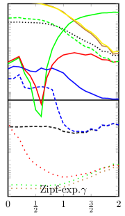
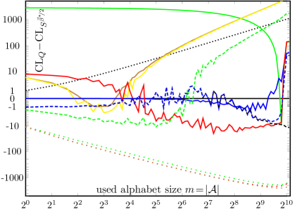
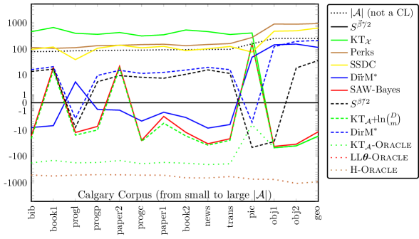
Figure 1: Plotted are code length differences to $S^{{\smash{\vec{\beta}^{*}\mskip-3.0mu}}\mskip-3.0mu/2}$ of various estimators. The two top graphs are for fixed sequence length $n=1024$ and total alphabet size $D=10\mskip 3.0mu000$ for varying Zipf exponents $\gamma$ and used alphabet sizes $m=|{\cal A}|$. The bottom graph is for the 14 files from the Calgary corpus with $21504\leq n\leq 768\mskip 3.0mu771$ and byte alphabet ($D=256$). The online/offline/oracle estimators have solid/dashed/dotted lines. A curve above/below zero means worse/better than $S^{{\smash{\vec{\beta}^{*}\mskip-3.0mu}}\mskip-3.0mu/2}$. The black dotted curve is not a code length but shows the used alphabet size $m\equiv|{\cal A}|$.

I determined the code length of various estimators for various sequence lengths $n$, used alphabet sizes $m$, and base alphabet sizes $D$ on artificially generated data sequences and the Calgary corpus. I consider the new estimator $S$ and the Dirichlet-multinomial with approximately optimal constant $\beta^{*}\mskip-3.0mu\mskip-3.0mu/2$ and variable ${\smash{\vec{\beta}^{*}\mskip-3.0mu}}\mskip-3.0mu/2$ and with Perks prior, the KT estimator for the base and for the used alphabet, and Bayesian sub-alphabet weighting, introduced in Section 7. I also compare against the true distribution and the empirical entropy.

Data generation. I sampled $\theta_{1},...,\theta_{m}$ uniformly from the $m-1$-dimensional probability simplex and set $\theta_{m+1}=...=\theta_{D}=0$. I then sampled $x_{1:n}$ from $P^{\boldsymbol{\theta}}_{iid}$. Unless $n\gg m$ or $D\gg n$, this usually results in sequences that actually contain less than $m$ symbols, and e.g. $|{\cal A}|=n$ is virtually impossible to achieve in this way. I therefore generate sequences by first setting $x_{t}=t$ for $t=1...\min\{m,n\}$, then sample the remaining $x_{t}$ from $P^{\boldsymbol{\theta}}_{iid}$, and then scramble the result. The resulting code lengths were virtually indistinguishable from the “normal” i.i.d. sampling, when the latter was also feasible.

I also generated sequences with a version of D’Hondt’s method for allocating seats in party-list proportional representation, which ensures $|n_{i}-\theta_{i}\cdot n|<1$ and adapted it to also ensure $n_{i}>0$ if $\theta_{i}>0$ and $i\leq n$ by dividing by zero (rather than 1) first. As expected, the results were a bit less noisy, but otherwise very similar.

In another experiment I chose $\boldsymbol{\theta}$ to be Zipf-distributed, i.e. $\theta_{i}\propto i^{-\gamma}$ with varying Zipf exponent $\gamma>0$, which for $\gamma\approx 1$ mimics quite well the empirical distribution of words in English texts. The larger $\gamma$, the smaller the used alphabet ${\cal A}$.

My $S$-estimators. I determined the code length of my models ($S^{\beta^{*}\mskip-3.0mu\mskip-3.0mu\mskip-3.0mu/2}$and $S^{{\smash{\vec{\beta}^{*}\mskip-3.0mu}}\mskip-3.0mu/2}$) with constant and variable optimal $\beta^{*}$. I chose uniform normalized weights $w^{t}_{i}=1/(D-m_{t})$. I also played around with other $\beta$ and $\vec{\beta}$, but performance either severely deteriorated, or only marginally and locally improved. The code length is very sensitive to some changes, e.g. $\beta=m/\ln n$ and $\beta=m/\ln{2n\over m}$ perform badly for large $m$, since these $\beta$ have the wrong scaling for $m\to n$, but less sensitive to other changes, e.g. $\beta=(m+c)/\ln{n+c^{\prime}\over m+c}$ for small $c,c^{\prime}$ are generally ok. For the experiments I used $\beta^{c=2}=\beta^{*}\mskip-3.0mu\mskip-3.0mu/2$ and $\beta^{c=2}_{t}=\beta^{*}_{t}/2$.

Other estimators. I also determined the code length of the other estimators discussed in Section 7. I considered:
(i) the Dirichlet-multinomial with $\boldsymbol{\alpha}=\boldsymbol{1}/D$ (Perks) and optimized constant $\boldsymbol{\alpha}^{*}$ ($\text{DirM}^{*}$) and optimal variable $\vec{\boldsymbol{\alpha}}^{*}$ (D$\vec{\smash{\rm i}}$rM^∗) with uniform weights (25);
(ii) the KT-estimator with base alphabet ${\cal X}$ ($\text{KT}_{\cal X}$),
(iii) the KT-estimator for used alphabet ${\cal A}$ ($\text{KT}_{\cal A}$-Oracle), a feasible off-line version by pre-coding ${\cal A}$ ($\text{KT}_{\cal A}\mskip-3.0mu+\mskip-3.0mu\ln{D\choose m}$), and the online version using escape probability ${{}^{1}\mskip-3.0mu/\mskip-3.0mu_{t+1}}$ (SSDC) discussed in Section 7;
(iv) the Bayesian sub-alphabet weighting (SAW-Bayes) discussed in Appendix G;
(v) the empirical entropy $nH({\boldsymbol{n}\over n})=\sum_{i}n_{i}\ln{n\over n_{i}}$ (H-Oracle);
(vi) the log-likelihood of the sampling distribution $\ln 1/P^{\boldsymbol{\theta}}_{iid}$ (LL$\boldsymbol{\theta}$-Oracle) for artificial data.

Results. Figure 1 plots the results for the various estimators. The vertical axis is the code length (or redundancy) difference of the estimator under consideration and our prime model $S^{{\smash{\vec{\beta}^{*}\mskip-3.0mu}}\mskip-3.0mu/2}$. So negative/positive values indicate better/worse performance than $S^{{\smash{\vec{\beta}^{*}\mskip-3.0mu}}\mskip-3.0mu/2}$. The two top graphs are for artificially generated data with fixed sequence length $n=1024$ and total alphabet size $D=10\mskip 3.0mu000$. In the right graph I varied $m=1,2,4,...2^{10}$ and in the left graph I varied the Zipf exponent $\gamma\in[0;2]$. The bottom graph shows results for the 14 files from the Calgary corpus with byte alphabet ($D=256$). All results are plotted and discussed relative to $S^{{\smash{\vec{\beta}^{*}\mskip-3.0mu}}\mskip-3.0mu/2}$. Rather than averaging over multiple runs and plotting error bars for the artificial data, I generated (necessarily) one new sequence for each $\gamma$ and $m$ for sufficiently many $\gamma$ and $m$. The noise level of the curves captures the sample variation very well.

Discussion. The results generally confirm the theory with few/small surprises.

The online estimators are plotted with solid lines. D$\vec{\smash{\rm i}}$rM^∗ mostly coincides within $\pm 10$ nits with $S^{{\smash{\vec{\beta}^{*}\mskip-3.0mu}}\mskip-3.0mu/2}$ for most $m$. Only when $m$ approached $n$ is $S^{{\smash{\vec{\beta}^{*}\mskip-3.0mu}}\mskip-3.0mu/2}$ superior to D$\vec{\smash{\rm i}}$rM^∗ due to renormalized weights leading to shorter $\text{CL}_{w}({\cal A})$. Among the proper estimators, SAW-Bayes works best by a small margin, except for very small ($m\lesssim\ln n$) and very large ($m\approx n$) used alphabet and Zipf distributed data, but note that it is $D$ (here $10\mskip 3.0mu000$ or 256) times slower than all the other algorithms. SSDC is virtually indistinguishable from Perks on the artificial data and only slightly better on the real data. Both perform poorly except for very small $m\lesssim\ln n$. Note that Perks performs as well as $\text{DirM}^{*}$ (only) around $m\approx 2\ln{n\over m}$, i.e. when their priors coincide. $\text{KT}_{\cal X}$ as well as $\text{DirM}^{\boldsymbol{\alpha}}$ with any other fixed choice of $\boldsymbol{\alpha}$ perform very badly, especially for small $m$. $\text{KT}_{\cal X}$ performs well only for $m\approx D$ and for $m\approx 0.9n$ when $\beta^{*}\mskip-3.0mu\mskip-3.0mu/2$ is accidentally close to $\alpha_{+}=D/2$.

The offline estimators (densely dashed lines), $\text{DirM}^{*}$, $S^{\beta^{*}\mskip-3.0mu\mskip-3.0mu\mskip-3.0mu/2}$ with constant optimal parameters $\boldsymbol{\alpha}^{*}$ and $\beta^{*}$ mostly coincide within $\pm 10$ nits with their variable $\vec{\boldsymbol{\alpha}}^{*}$ and ${\smash{\vec{\beta}^{*}\mskip-3.0mu}}$ online versions, except for very large $m$ they are slightly better. This shows that making them online is essentially for free, which is consistent with the close bounds for small $m$ in both cases. This has been observed for other offline-online algorithm pairs as well [HP05]. There is very little gain in knowing $\boldsymbol{\alpha}^{*}$ or $\beta^{*}$ in advance. As expected off-line $\text{KT}_{\cal A}\mskip-3.0mu+\mskip-3.0mu\ln{D\choose m}$ significantly improves upon $\text{KT}_{\cal X}$ for small $m$ and even beats $S^{{\smash{\vec{\beta}^{*}\mskip-3.0mu}}\mskip-3.0mu/2}$ by a couple of bits for sufficiently small $m$, but breaks down for medium and large $m$, and anyway is off-line.

These observations are rather consistent across uniform, Zipf, and real data. Only for Zipf data, SAW-Bayes and $\text{KT}_{\cal A}\mskip-3.0mu+\mskip-3.0mu\ln{D\choose m}$ seem to be worse, and the relative performance of many estimators on b&w fax pic is reversed.

The oracle estimators (dotted lines) possess significant extra knowledge: $\text{KT}_{\cal A}$-Oracle the used alphabet ${\cal A}$, and LL$\boldsymbol{\theta}$-Oracle and H-Oracle even the counts $\boldsymbol{n}$. The plots show the magnitude of this extra knowledge.

Summary. Results are similar for other $(n,D,m)$ and $(n,D,\gamma)$ combinations but code length differences can be more or less pronounced but are seldom reversed. In short, $\text{KT}_{\cal X}$ performs very poorly unless $m\approx D$, and Perks and SSDC perform poorly unless $m\lesssim\ln n$; $\text{KT}_{\cal A}\mskip-3.0mu+\mskip-3.0mu\ln{D\choose m}$, $\text{DirM}^{*}$, $S^{\beta^{*}\mskip-3.0mu\mskip-3.0mu\mskip-3.0mu/2}$ are not online; the oracles LL$\boldsymbol{\theta}$-Oracle, H-Oracle, $\text{KT}_{\cal A}$-Oracle are not realizable; and SAW-Bayes is extremely slow; which leaves D$\vec{\smash{\rm i}}$rM^∗ and $S^{{\smash{\vec{\beta}^{*}\mskip-3.0mu}}\mskip-3.0mu/2}$ as winners. They perform very similar unless $m$ gets very close to $\min\{n,D\}$ in which case $S^{{\smash{\vec{\beta}^{*}\mskip-3.0mu}}\mskip-3.0mu/2}$ wins.

Appendix J List of Notation

Symbol	Explanation
${\cal X}$	total (large) base alphabet of size $D$
$D=|{\cal X}|$	size of (large) base alphabet ${\cal X}$
$n$	sequence length
$x_{1:n}$	total sequence
$n_{i}$	number of times $i$ appears in $x_{1:n}$
${\cal A}\subseteq{\cal X}$	symbols actually appearing in sequence $x_{1:n}$
$m=|{\cal A}|$	size of alphabet used in $x_{1:n}$
$i,j,k$	indices ranging over symbols in ${\cal X}$, ${\cal A}$, ${\cal X}\setminus{\cal A}$ respectively
$\bar{\nu}:={n\over m},\nu:={m\over n}$	average multiplicity of symbols and its inverse
$t$	current time ranging from $0$ to $n-1$
$x_{1:t}$	sequence seen so far
${\cal A}_{t}$	$=\{x_{1},...,x_{t}\}$ = symbols seen so far
$m_{t}=|{\cal A}_{t}|$	number of different symbols observed so far (in $x_{1:t}$)
$x_{t+1}$	next symbol to be predicted
$n^{t}_{i}$	number of times $i$ appears in $x_{1:t}$
${\cal N}\mskip-3.0mu\text{\it ew}$	set of $t$ for which $x_{t+1}$ is new, i.e. $x_{t+1}\not\in{\cal A}_{t}$
${\cal O}\text{\it ld}$	set of $t$ for which $x_{t+1}$ is old, i.e. $x_{t+1}\in{\cal A}_{t}$
$P,Q$	probability over sequences
$P^{\rm param}_{\rm name}$	parameterized and named probability
$R^{\rm param}_{\rm name}$	$=-\ln P^{\rm param}_{\rm name}-n\cdot H(\boldsymbol{n}/n)$ = redundancy of $P^{\rm param}_{\rm name}$
$\overline{R},\underline{R}$	upper/lower bound on redundancy
CL	code length in nits
$\theta_{i}$	probability that $x_{t}=i$
$\@tabbing@_i,\@tabbing@_+$	Dirichlet parameters and their sum
$\beta=\beta_{n},\beta_{t}$	general (constant,variable) parameter $\beta$
$\beta^{*}\neq\beta^{*}_{n},\beta^{*}_{t}$	optimal (constant,variable) parameter $\beta$
$w^{t}_{i}$	weight of new symbol $i$ at time $t$
$\ln$	Natural logaritm. Results are in ‘nits’
$\boldsymbol{v}$	vector over alphabet ${\cal X}$
$\vec{v}$	vector over time $t=0...n-1$
$\Gamma,\Psi$	Gamma and diGamma function
$c$	constant $>0$ and $<\infty$

References

• [Bay63] T. Bayes. An essay towards solving a problem in the doctrine of chances. Philosophical Transactions of the Royal Society, 53:370–418, 1763. [Reprinted in Biometrika, 45, 296–315, 1958].
• [Ber79] J. M. Bernardo. Reference posterior distributions for Bayesian inference (with discussion). Journal of the Royal Statistical Society, B41:113–147, 1979.
• [BEY06] R. Begleiter and R. El-Yaniv. Superior guarantees for sequential prediction and lossless compression via alphabet decomposition. Journal of Machine Learning Research, 7:379–411, 2006.
• [BH10] W. Buntine and M. Hutter. A Bayesian view of the Poisson-Dirichlet process. Technical Report arXiv:1007.0296, NICTA and ANU, Australia, 2010.
• [Bis06] C. M. Bishop. Pattern Recognition and Machine Learning. Springer, 2006.
• [CT06] T. M. Cover and J. A. Thomas. Elements of Information Theory. Wiley-Intersience, 2nd edition, 2006.
• [CW84] J. G. Cleary and I. H. Witten. Data compression using adaptive coding and partial string matching. IEEE Transactions on Communications, COM-32(4):396–402, 1984.
• [Fin74] B. de Finetti. Theory of Probability : A Critical Introductory Treatment. Wiley, 1974. Vol.1&2, transl. by A. Machi and A. Smith.
• [Grü07] P. D. Grünwald. The Minimum Description Length Principle. The MIT Press, Cambridge, 2007.
• [Hal48] J. B. S. Haldane. The precision of observed values of small frequencies. Biometrika, 35:297–300, 1948.
• [HP05] M. Hutter and J. Poland. Adaptive online prediction by following the perturbed leader. Journal of Machine Learning Research, 6:639–660, 2005.
• [Hut03] M. Hutter. Optimality of universal Bayesian prediction for general loss and alphabet. Journal of Machine Learning Research, 4:971–1000, 2003.
• [Jef46] H. Jeffreys. An invariant form for the prior probability in estimation problems. In Proc. Royal Society London, volume Series A 186, pages 453–461, 1946.
• [Jef61] H. Jeffreys. Theory of Probability. Clarendon Press, Oxford, 3rd edition, 1961.
• [Kri98] R. E. Krichevskiy. Laplace’s law of succession and universal encoding. IEEE Transactions on Information Theory, 44(1):296–303, 1998.
• [KT81] R. Krichevsky and V. Trofimov. The performance of universal encoding. IEEE Transactions on Information Theory, 27(2):199–207, 1981.
• [Lap12] P. Laplace. Théorie analytique des probabilités. Courcier, Paris, 1812. [English translation by F. W. Truscott and F. L. Emory: A Philosophical Essay on Probabilities. Dover, 1952].
• [Mah12] M. Mahoney. Data Compression Explained. Dell, Inc, http://mattmahoney.net/dc/dce.html, 2012.
• [MS99] C. D. Manning and H. Schütze. Foundations of Statistical Natural Language Processing. MIT Press, 1999.
• [OHSS12] A. O’Neill, M. Hutter, W. Shao, and P. Sunehag. Adaptive context tree weighting. In Proc. Data Compression Conference (DCC’12), pages 317–326, Snowbird, Utah, USA, 2012. IEEE Computer Society.
• [Per47] W. Perks. Some observations on inverse probability including a new indifference rule. Journal of the Institute of Actuaries, 73:285–334, 1947.
• [Ris76] J. J. Rissanen. Generalized Kraft inequality and arithmetic coding. IBM Journal of Research and Development, 20(3):198–203, 1976.
• [Ris84] J. J. Rissanen. Universal coding, information, prediction, and estimation. IEEE Transactions on Information Theory, I(4):629–636, 1984.
• [Sha48] C. E. Shannon. A mathematical theory of communication. Bell System Technical Journal, 27:379–423, 623–656, 1948.
• [TSW93] T. J. Tjalkens, Y. M. Shtarkov, and F. M. J. Willems. Sequential weighting algorithms for multi-alphabet sources. Proc. 6th Joint Swedish-Russian Intl. Workshop on Information Theory, pages 22–27, 1993.
• [VH12] J. Veness and M. Hutter. Sparse sequential Dirichlet coding. Technical Report arXiv:1206.3618, UoA and ANU, 2012.
• [VNHB12] J. Veness, K. S. Ng, M. Hutter, and M. Bowling. Context tree switching. In Proc. Data Compression Conference (DCC’12), pages 327–336, Snowbird, Utah, USA, 2012. IEEE Computer Society.
• [Wal05] C. S. Wallace. Statistical and Inductive Inference by Minimum Message Length. Springer, Berlin, 2005.
• [WNC87] I. H. Witten, , R. M. Neal, and J. G. Cleary. Arithmetic coding for data compression. Communications of the ACM, 30(6):520–540, 1987.