Fighting against uncertainty:
An essential issue in bioinformatics

Abstract

Many bioinformatics problems, such as sequence alignment, gene prediction, phylogenetic tree estimation and RNA secondary structure prediction, are often affected by the “uncertainty” of a solution; that is, the probability of the solution is extremely small. This situation arises for estimation problems on high-dimensional discrete spaces in which the number of possible discrete solutions is immense. In the analysis of biological data or the development of prediction algorithms, this uncertainty should be handled carefully and appropriately. In this review, I will explain several methods to combat this uncertainty, presenting a number of examples in bioinformatics. The methods include (i) avoiding point estimation, (ii) maximum expected accuracy (MEA) estimations, and (iii) several strategies to design a pipeline involving several prediction methods. I believe that the basic concepts and ideas described in this review will be generally useful for estimation problems in various areas of bioinformatics.

1 Introduction

1.1 Uncertainty of solutions

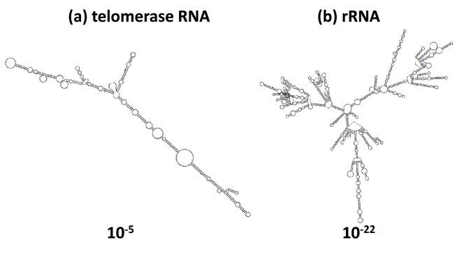
In estimation problems that appear in bioinformatics, such as sequence alignment [1], gene prediction [2], RNA secondary structure prediction [3, 4], RNA-RNA interaction prediction [5], and phylogenetic tree estimation [6], it is typical that the probability of any solution is extremely small even if that solution has the highest probability. For example, the probabilities of the minimum free energy (MFE) structures of a telomerase RNA and a ribosomal RNA are $8\times 10^{-6}$ and $4\times 10^{-23}$, respectively (Figure 1). Here the probabilities were computed by using the Boltzmann distribution (also called the Gibbs distribution) from statistical mechanics [9]:

$$p(\theta|x)=\frac{1}{Z(x)}\exp\left(\frac{-E(\theta,x)}{RT}\right)$$ (1)

where $\theta$ is a specific secondary structure (e.g., the MFE structure) of an RNA sequence $x$, $E(\theta,x)$ is the free energy of secondary structure $\theta$, $T$ is the temperature, $R$ is the ideal gas constant (8.31 J/mol K) and $Z(x)$ is the normalizing constant (partition function) that ensures $\sum_{\theta}p(\theta|x)=1$. The situation is much worse in the problem of RNA deleterious mutation prediction [10, 11, 12], in which a specific RNA secondary structure is sought from among all possible secondary structures with up to $k$ mutations and the partition function thus becomes much larger (cf. see Figure 4 in Barash and Churkin [10]).

The fact that the probability of a solution can be extremely small is known as the uncertainty of solutions, which leads to a critical issue in developing prediction algorithms or analyzing biological data in the field of bioinformatics [13, 14, 15, 16, 17]. In one Science paper [15], for instance, the authors argued that the uncertainty of multiple sequence alignment greatly influences phylogenetic topology estimations: phylogenetic topologies estimated from multiple alignments predicted by 5 widely used aligners are different from one another. There is no doubt that this raises serious issues for reaching biological conclusions.

Figure 1: The probabilities of forming the minimum free energy (MFE) structure, computed by using the Boltzmann distribution (see Eq 1), for (a) telomerase RNA and (b) ribosomal RNA. Note that both probabilities are the highest ones among all possible secondary structures for each RNA, because the structures have the minimum free energy of all possible structures.

1.2 Where does the uncertainty come from?

The uncertainty described in the previous section arises for estimation problems on high-dimensional discrete spaces, in which the number of possible solutions is immense. For instance, the following results for the asymptotic number of solutions in particular problems are known:

• The number of possible secondary structures, $S(n)$, of an RNA sequence with length $n$ is estimated to be

  $$S(n)\sim\sqrt{\frac{15+7\sqrt{5}}{8\pi}}n^{-1.5}\left(\frac{3+\sqrt{5}}{2}\right)^{n}$$

  where $f(n)\sim g(n)$ means that $\lim_{n\to\infty}f(n)/g(n)=1$. See Theorem 13.2 in [18] for the proof.

• Let $f(n,m)$ be the number of alignments of one sequence of $n$ letters with another of $m$ letters. Then $f(n,n)$ is estimated to be

  $$f(n,n)\sim(1+\sqrt{2})^{2n+1}n^{-1/2}.$$

  See Theorem 9.1 in [18] for the proof.

• The number of topologies of a phylogenetic tree (un-rooted binary tree) with $n(>3)$ leaves (formally called “operational taxonomy units”) is $\prod_{j=3}^{n}(2j-5)=1\cdot 3\cdot 5\cdot\cdots\cdot(2n-5)$. See Proposition 14.1 in [18] for the proof.

In the equations above, the number of solutions increases exponentially with $n$ so, for example, the number of alignments of two sequences with length 1000 is $f(1000,1000)\sim 10^{767.4\ldots}$, which is immense because it has been estimated that the number of particles in the universe is about $10^{80}$. Because the sum of the probabilities of all solutions must be equal to 1, the probability of any particular solution tends to become extremely small because of the large number of potential solutions. In addition, there often exist many very-similar solutions: for a given RNA secondary structure $s$, secondary structures produced by unpairing a base-pair (in $s$) are similar to the original secondary structure.

1.3 Purpose of this review

In this review, I aim to introduce several methods to handle this uncertainty appropriately in the field of bioinformatics, presenting a number of actual studies. Most examples are adopted from either RNA informatics or sequence alignments. The methods include (i) avoiding point estimation (e.g., prediction of suboptimal solutions), (ii) maximum expected accuracy (MEA) estimations, and (iii) several strategies to design a pipeline involving several prediction methods.

Throughout this article, the following notation and definitions are used.

• $Y$ denotes a predictive (solution) space, including all the possible solutions that are discrete. For example, $Y$ is the set of possible RNA secondary structures of an RNA sequence $x$.

• $p(\theta|D)$ denotes a posterior probability distribution on a predictive space $Y$, given data $D$. For example, $p(\theta|x)$ is a probability distribution of secondary structures of an RNA sequence $D=\{x\}$ given by Eq. (1). In this study, I will just assume the existence of this probability distribution on the predictive space in most cases.

• Predicting one solution from the predictive space $Y$ is called a point estimation. The probability of the solution found by point estimation is sometimes extremely low as described in the previous section.

This paper is organized as follows. In Section 2, I describe methods to avoid point estimation by sampling several sub-optimal solutions or visualizing the distribution of solutions. In Section 3, I introduce methods to predict one solution, taking the uncertainty into account, because there are several situations in which only one solution is required. In Section 4, I give some strategies for developing complex pipelines or algorithms in which several prediction methods are involved. In Section 5 these approaches are discussed and the direction of future research in areas related to this study is considered.

2 Avoiding point estimations

2.1 Prediction of suboptimal solutions

One possible method to handle the uncertainty described in Section 1 is to predict not only the one optimal solution but also several sub-optimal solutions. Zuker [19], in a study of RNA secondary structure prediction, was the first to introduce a method to predict suboptimal solutions, implemented in Mfold [20] (See Supplementary Section A for the details).

2.1.1 Stochastic sampling with dynamic programming

Stochastic sampling (SS) in combination with a dynamic programming (DP) technique enables the efficient sampling of solutions from a distribution $p(\theta|D)$ of solutions. For both RNA secondary structure predictions and pairwise alignments, stochastic sampling is realized by stochastically conducting a traceback procedure in a DP algorithm [1, 21]. For example, RNAsubopt [22] predicts the complete set of suboptimal secondary structures within a given energy range (say, 1 kcal/mol) from the minimum free energy.

2.1.2 MCMC and Gibbs sampling

For a probability distribution whose probabilistic structure is more complicated, a Markov-chain Monte-Carlo (MCMC) algorithm [23], such as Gibbs sampling, is a widely applicable method to sample from the posterior distribution, although in most applications MCMC is used to obtain the optimized solution.

Meyer et al. [24] applied an MCMC method to optimize the joint probability distribution

$$P(S,A,T|D)=\frac{1}{Z}P(D|S,A,T)P(S,A,T)$$ (2)

where $D$ stands for the data (i.e., unaligned RNA sequences), $Z=P(D)$ is a normalizing constant (partition function), $S$ is a consensus (or common) RNA secondary structure that might contain pseudoknots, $A$ is a multiple sequence alignment, and $T$ is an evolutionary tree relating the sequences. It would be difficult not only to optimize this posterior probability using dynamic programming techniques but also to apply stochastic sampling with a dynamic programming described in the previous section, because the probability structures are complex joint distributions of three states.

Metzler and Nebel [25] and Bon et al. [26] proposed a probabilistic model for RNA secondary structures with pseudoknots and presented an MCMC Method for sampling RNA structures according to their posterior distribution for a given sequence. In contrast to conventional RNA secondary structure prediction (which does not consider pseudoknots), RNA secondary structure prediction with pseudoknots entails a larger computational cost (see [27]) and the application of stochastic sampling is not realistic. Doose and Metzler [28] presented a method (PhyloQfold) that takes advantage of the evolutionary history of a group of aligned RNA sequences for sampling consensus secondary structures, including pseudoknots, according to their approximate posterior probability. Wei et al. [29] presented a new global structural alignment algorithm, RNAG, to predict consensus secondary structures for unaligned sequences, utilizing a blocked Gibbs sampling algorithm.

For phylogenetic tree estimations, MrBayes [30] is a program for Bayesian phylogenetic analysis, which uses MCMC techniques to sample from the posterior probability distribution of phylogenetic trees for a given multiple sequence alignment. More recently, the program BigFoot [31] employed an MCMC method for finding joint distributions of phylogenetic trees and multiple sequence alignments (MSA).

As shown by the above examples, MCMC and Gibbs sampling seem useful methods to sample suboptimal solutions when the structure of target probability distribution is complex.

2.1.3 Non-stochastic approaches

Typically, the approach described in the previous sections returns a huge number of secondary structures in which there are many structures that are similar to each other (cf. Figure 2). To overcome this, a method to predict representative suboptimal secondary structures, such as locally optimal secondary structures or alignments, has been proposed [19, 32, 33] (cf. Supplementary Section A). Moreover, for RNA secondary structure predictions, RNAshapes [34] implements an algorithm to predict secondary structures for every abstract shape, which is realized by using an algebraic dynamic programming (ADP) technique [35]. This reduces the number of predictions (Figure 3). Note that a probabilistic version of RNAshapes has also been proposed, which computes the accumulated probabilities of all structures that share a shape [36].

Figure 2: Suboptimal secondary structures of a tRNA sequence predicted by RNAsubopt [22], enumerating all possible suboptimal RNA secondary structures within a given energy range from the minimum free energy (MFE).

Figure 3: RNAshapes (http://bibiserv.techfak.uni-bielefeld.de/rnashapes/) [34] results for secondary structures of a tRNA sequence. The rightmost structures of each secondary structure with ‘[’ and ‘]’ are abstract shapes, which represent coarse-grain secondary structures. RNAshapes predicts only one optimal secondary structure for each abstract shape, reducing the number of predictions.

2.1.4 Prediction of representative solutions after clustering

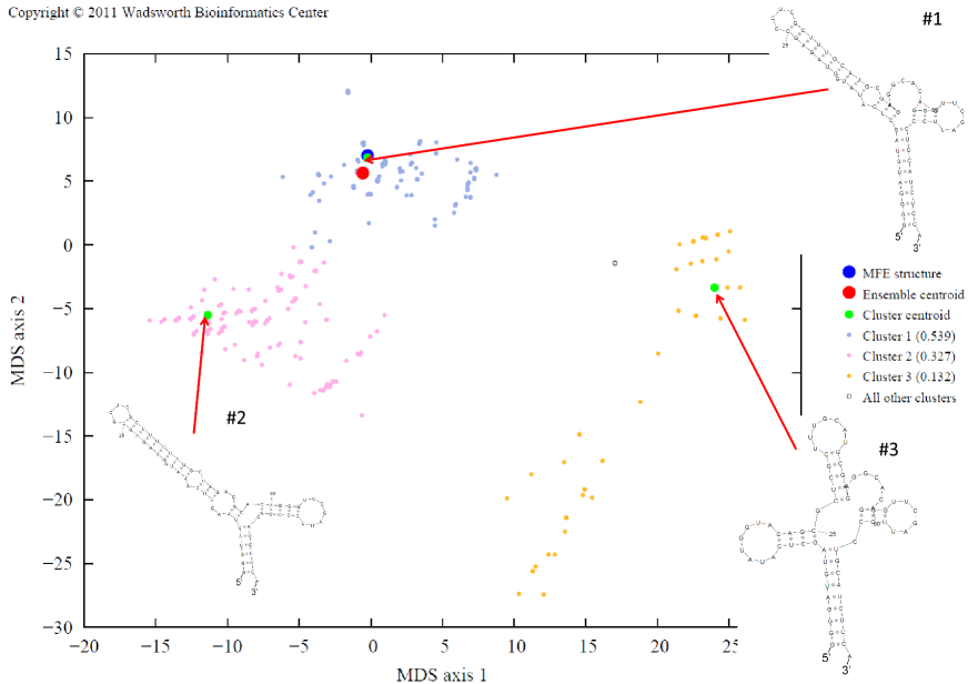
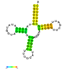
In this approach, first stochastic sampling (Section 2.1.1) is performed, then the suboptimal solutions are clustered, and finally a solution for each cluster is predicted. In this way, it is expected that a diverse variety of solutions (i.e., solutions are not similar to each other) will be obtained. For RNA secondary structure predictions, this approach is implemented in Sfold [37] and CentroidFold [38], Sfold provides a Web-interface for this approach (http://sfold.wadsworth.org/cgi-bin/index.pl). See Figure 4 for an example of the output of the Sfold Web Server for a typical tRNA sequence.

Figure 4: Clustering result from the Sfold Web Server (http://sfold.wadsworth.org/) [37]. A tRNA sequence was used to draw this figure. The space of secondary structures is embedded into two dimensional space using Multidimensional distance scaling [39] (the center plot) on the base-pair distance of RNA secondary structures. Four secondary structures are shown, corresponding to the centroid structures for the 1st, 2nd and 3rd clusters, respectively.

2.2 Visualizing distributions of solutions

Visualization of the distribution of solutions would include much richer information than a single solution. Yet, visualizing solutions is not trivial because the solution space is generally high-dimensional (cf. Section 1.2).

2.2.1 Visualizing distributions of solutions with sampling

In many cases, a solution lies in a high-dimensional discrete space and the number of possible solutions is immense; it is therefore difficult to visualize solutions directly. To address this, multidimensional distance scaling (MDS) [39] or principal component analysis (PCA) is utilized in combination with the sampling of solutions by stochastic sampling or MCMC.

For RNA secondary structure predictions, Sfold produces this kind of visualization of a distribution of RNA secondary structures in terms of base-pair distance (Figure 4).

For phylogenetic tree estimations, Amenta and Klingner [40] and Hillis et al. [41] proposed a method to visualize phylogenetic trees by utilizing MDS based on a distance between two phylogenetic trees, called the Robinson-Foulds (RF) distance [42] (the sum of the internal edges in disagreement between the two trees). More recently, Huang and Li [43] have developed some software MASTtreedist that employs MDS with the maximum agreement subtree (MAST) distance, which is the number of leaves in common for the maximum subtree between the two trees [44]. This leads to better clustering results than using the RF distance.

2.2.2 Visualizing distributions with one or two reference solutions

Instead of visualizing the distribution of solutions directly (Section2.2.1), it has been proposed to visualize the distribution with one or two reference solutions. Let us first consider a reference case, in which one reference solution $s_{0}$ and a distance, $d(\cdot,\cdot)$, between two solutions are given. For each integer value $k$, $p(k)$ is equal to the sum of probabilities for solutions whose distance from $s_{0}$ is equal to $k$:

$$p(k)=\sum_{s^{\prime}\in\{s|d(s_{0},s)=k\}}p(s^{\prime}|D)$$

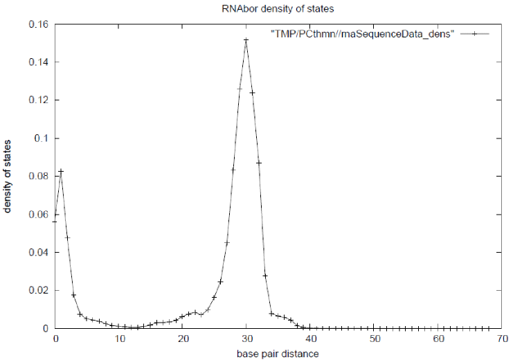
where $p(\cdot|D)$ is a probability distribution over solutions. Then, the distribution $p(k)$ ($k=1,2,3,\cdots$) can be easily visualized. One advantage of this visualization is that, for several problems such as alignments and RNA secondary structure predictions, the distribution can be computed exactly by employing dynamic programming techniques (Newberg and Lawrence [45]). The programs RNAbor [46, 47] and RNAborMEA [48] implement this approach. Figure 5 shows an example of RNAbor results for a 101 nucleotide SAM riboswitch. It should be noted that points with a large base-pair distance from the reference structure may include a lot of structures which might be very different from each other.

This approach can be extended to two (or more) solutions. If two reference solutions $s_{0}$ and $s_{1}$ are given, the distribution $p(k,l)$ ($k,l=1,2,\cdots$) is defined by

$$p(k,l)=\sum_{s^{\prime}\in\{s|d(s_{0},s)=k\wedge d(s_{1},s)=k\}}p(s^{\prime}|D).$$

In this case, the distribution becomes more specific and includes richer information than that with one reference case. The entire distribution $p(k,l)$ with two reference solutions can be efficiently computed by using dynamic programming for RNA secondary structures and alignments [49].

Recently, a more efficient method for visualization of both one and two reference cases has been proposed. This method uses a discrete Fourier transform (DFT) and parallel computing (Mori et al., manuscript in preparation).

Figure 5: The result of RNAbor for a 101 nucleotide SAM riboswitch sequence from the Rfam database [50], with EMBL accession code AP004597.1/118941-119041: UACUUAUCAAGAGAGGUGGAGGGACUGGCCCGCUGAAACCUCAGCAACAGAACGCAUCUGUCUGUGCUAAAUCCUGCAAGCAAUAGCUUGAAAGAUAAGUU. The secondary structure corresponding to the origin is the reference structure in the Rfam database. The horizontal axis indicates base-pair distance [37], and the vertical axis indicates probability density of RNA secondary structures whose base-pair distance is equal to the value on the horizontal axis.

2.3 Visualizing marginal probabilities

Marginal probabilities are the sums of probabilities of solutions that satisfy a specific condition, and are formally represented by

$$p_{\mathcal{C}}=\sum_{\theta\in\mathcal{C}}p(\theta|D)$$ (3)

where $\mathcal{C}$ is a subset of the predictive space $Y$ satisfying a condition of interest. Marginal probabilities with respect to an appropriate condition are often much larger (typically, near to 1) than the probability of a solution itself (which is, typically, less than $10^{-5}$; see Figure 1), and visualization of marginalized probabilities includes rich information, as shown in the following examples.

Example 1 (Base-pairing probabilities (BPPs))

A base-pairing probability (BPP), $p_{ij}$, of an RNA sequence $x$ is the marginal probability that $x_{i}$ and $x_{j}$ (the $i$-th and $j$-th nucleotides of $x$) form a base-pair:

$$p_{ij}=\sum_{\theta\in\mathcal{C}(i,j)}p(\theta|x)$$ (4)

where $\mathcal{C}(i,j)$ is a set of secondary structures whose $i$-th position forms a base-pair with the $j$-th position, and $p(\theta|x)$ is a probability distribution of secondary structures of $x$, for example, given by the McCaskill model [9] (cf. Eq. (1)).

The set of all base-pairing probabilities for all pairs of nucleotides in a given RNA sequence is called a “base-pairing probability matrix” (BPPM), and is represented as a triangular matrix $P=\{p_{ij}\}_{1\leq i<j\leq|x|}$ where $p_{ij}\in[0,1]$ is defined in Eq. (4). The BPPM of typical models for RNA secondary structures can be computed in a polynomial order time by employing a dynamic programming algorithm (e.g., see [9]).

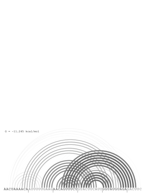
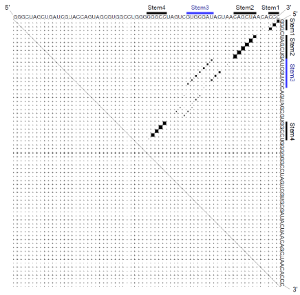
In Figure 6, the base-pairing probability matrix for an RNA aptamer is shown. Notice that, although the base-pairing probability matrix does not specify a secondary structure, it includes richer information about structures than can be obtained from a single RNA secondary structure. See Section 5.1.1 for the details.

Recently, other visualizations of base-pairing probabilities have been proposed (RNABow [51]; http://rna.williams.edu/rnabows/single.html). See Supplementary Figure S2 for an example of RNABow output.

Figure 6: A base-pairing probability matrix for an RNA aptamer [52]. See Figure 13 for the detailed implication of it. by biochemical experiments.

Example 2 (Aligned-pairing probabilities (APPs))

An aligned-pairing probability (APP), $p_{ik}$, of two sequences $x$ and $x^{\prime}$ gives the probability that $x_{i}$ and $x^{\prime}_{k}$ align:

$$p_{ik}=\sum_{\theta\in\mathcal{C}(i,k)}p(\theta|x,x^{\prime})$$ (5)

where $\mathcal{C}(i,k)$ is the set of pairwise alignments whose $i$-th base (nucleotide or amino acid) in $x$ aligns with the $k$-th base in $x^{\prime}$, and $p(\theta|x,x^{\prime})$ is a probability distribution for pairwise alignments between $x$ and $x^{\prime}$, such as the Miyazawa model [53] or pair hidden Markov models (pHMMs) [1].

The entire set of probabilities for every possible pair of base alignments between two sequences $x$ and $x^{\prime}$ is called an “aligned-pairing probability matrix” (APPM), It is represented by a matrix $P=\{p_{ik}\}_{1\leq i\leq|x|,1\leq|x^{\prime}|\leq k}$ where $p_{ik}\in[0,1]$ is defined in Eq. (5). The APPM of typical models for pairwise alignments can be computed in polynomial order time by employing a dynamic programming algorithm (See, e.g., Durbin et al. [1]. Like a BPPM for an RNA sequence, an APPM can be easily visualized.

Example 3 (Leaf splitting probabilities)

A leaf splitting probability, $p_{X,Y}$, for a leaf set $S$ gives the marginal probability that there exists a partition $(X,Y)$ of $S$ (i.e., $X\cup Y=S$ and $X\cap Y=\emptyset$) formed by cutting an internal edge in a phylogenetic tree:

$$p_{X,Y}=\sum_{\theta\in\mathcal{C}(X,Y)}p(\theta|S)$$ (6)

where $C(X,Y)$ is the set of phylogenetic tree topologies that can be split into $X$ and $Y$ by cutting one edge in $T$, and $p(\theta|S)$ is a probability distribution of phylogenetic tree topologies, such as the one given in [30].

Unlike base-paring probabilities or aligned-pairing probabilities, it is difficult to visualize the complete set of splitting probabilities because it cannot be represented as a “matrix”. The following is a non-trivial visualization of phylogenetic trees, with leaf splitting probabilities.

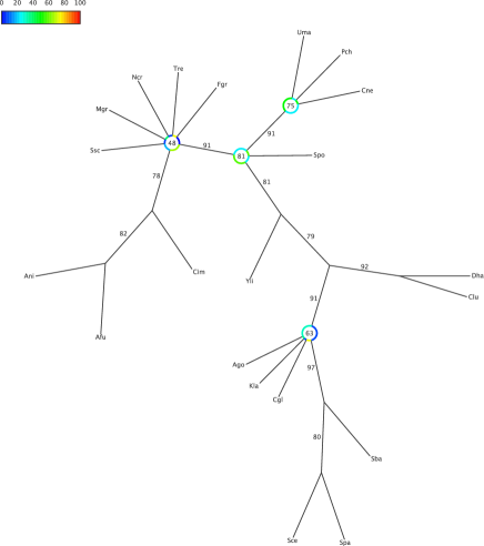
Example 4 (Centroid Wheel Tree (CWT) [54])

For phylogenetic tree estimations, a Centroid Wheel Tree (CWT) [54] provides a novel visualization of a phylogenetic tree topology with marginal probabilities (leaf splitting probabilities; Example 3). See Figure 7 for an example. See [54] for the detailed definition and algorithms for computing a CWT. A CWT can be computed through a Web site (http://cwt.cb.k.u-tokyo.ac.jp/).

Figure 7: An example of a Centroid Wheel Tree (CWT) computed using the Web site: http://cwt.cb.k.u-tokyo.ac.jp/. In this representation, leaf splitting probabilities are shown next to each edge.

3 What should we do when one prediction is required?

Although the approaches described in the previous section are good ways to handle uncertainty, it is often necessary to predict only one solution.

3.1 Maximum likelihood estimator and its drawback

A straight-forward approach to make a prediction for a given probability distribution, $p(y|D)$, on the predictive space $Y$ is to find the solution $\hat{y}$ with the maximum probability:

$$\hat{y}=\mathop{\mathrm{argmax}}_{y\in Y}p(y|D).$$ (7)

This approach is known as maximum likelihood (ML) estimation. Many existing tools or algorithms employ ML estimators; however, recent studies have indicated that ML estimators are not always superior estimators e.g. [55, 56]. The following is a typical example in which the ML estimator is inappropriate.

Example 5 (Carvalho and Lawrence [55])

The predictive space is the $n$-dimensional binary space $Y=\{0,1\}^{n}$, in which similar vectors in $Y$ represent similar predictions. We introduce a probability distribution on $Y=\{0,1\}^{n}$ as follows:

$$p(\theta|D)=\left\{\begin{array}[]{ll}p_{1}:=\frac{1}{n+3}&\mbox{if }\theta\in\mathcal{S}:=\left\{(x_{1},\ldots,x_{n})|x_{k}\in\{0,1\},\sum_{k=1}^{n}x_{k}\leq 1\right\}\\ p_{2}:=\frac{2}{n+3}&\mbox{if }\theta=\theta^{1}:=(1,1,\ldots,1)\\ 0&\mbox{otherwise}\end{array}\right.$$

(Clearly, $\sum_{\theta\in Y}p(\theta|D)=1$.) Then, the maximum likelihood estimator gives the solution $\theta^{1}=(1,1,\ldots,1)$. However, it can be seen that

$$\sum_{\theta:H(\theta^{0},\theta)\leq 1}p(\theta|D)=\frac{n+1}{n+3}$$

where $\theta^{0}$ is the zero vector in $\{0,1\}^{n}$ (i.e., all elements in the vector are equal to 0) and $H(\cdot,\cdot)$ is the Hamming distance. This means that, when $n=997$, the sum of the probabilities solutions around (similar to) $\theta^{0}$, for which the Hamming distance from $\theta^{0}$ is less than or equal to 1, is 0.998, while the probability of the ML estimation (i.e., $\theta^{1}$) is only 0.002 (Figure 8), indicating that $\theta^{0}$ is a much better estimation than the ML estimation $\theta^{1}$. Note that the ML estimation $\theta^{1}$ is a long way from the solution $\theta^{0}$ because $H(\theta^{0},\theta^{1})=n$.

Figure 8: An example of Carvalho and Lawrence [55], indicating that the ML estimation may not be very good. In this example, the predictive space is the $n$-dimensional binary space, $Y=\{0,1\}^{n}$, and we assume that similar binary vectors give similar predictions. Probabilities of each solution are shown in the figure (see the main text for the details) and edges are shown between solutions whose Hamming distance is 1 The ML estimation is $\theta^{1}$ but the sum of probabilities around $\theta^{0}$ is much larger than the probability of $\theta^{1}$. See Example 5 in the main text for the details.

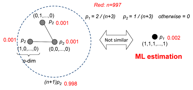
It is worth noting that several bioinformatics problems (including RNA secondary structure prediction, RNA-RNA interaction prediction, sequence alignment, and phylogenetic tree estimation) can be formulated as a point estimation problem in (a subset of) binary spaces $Y=\{0,1\}^{n}$ with large $n$ [56]. Hence, a similar situation to the one in the above (artificial) example could occur in real problems in bioinformatics. (For example, in Figure 4, the clover-leaf structure of tRNA does not lie in the 1st rank cluster.)

3.2 Maximum expected gain/accuracy (MEG/MEA) estimators

Because ML estimators are not always good estimators, as shown in Example 5, we will introduce alternatives to ML estimators in this section, on the basis of given accuracy/evaluation measures for the prediction problem.

3.2.1 Definition

Given a probability distribution $p(\theta|D)$ on a predictive space $Y$, the maximum expected gain (MEG) estimator is defined by

$$\hat{y}=\mathop{\mathrm{arg\ max}}_{y\in Y}\sum_{\theta\in Y}G(\theta,y)p(\theta|D)$$ (8)

where $G(\theta,y)$ is called the gain function, which returns the similarity between two solutions in $Y$. When the gain function is designed according to an accuracy or evaluation measure for the target problem, in which $y$ and $\theta$ are considered as a prediction and reference, respectively, the estimator is often called a maximum expected accuracy (MEA) estimator [57, 58, 59]. MEA estimators predict the solution by maximizing the expected accuracy when the solutions are distributed according to $p(\theta|D)$. These estimates are, therefore, appropriate for the given accuracy measure.

3.2.2 ML estimators from the viewpoint of MEA

Let us consider the ML estimator from the viewpoint of MEA. The ML estimator of Eq. (7) can be represented as

$$\hat{y} =\mathop{\mathrm{arg\ max}}_{y\in Y}p(y|D)$$

$$=\mathop{\mathrm{arg\ max}}_{y\in Y}\sum_{\theta\in Y}\delta(\theta,y)p(\theta|D)$$

where $\delta(\theta,y)$ is the Kronecker delta function that returns 1 only if $\theta=y$. This means the ML estimator is a kind of MEG/MEA estimator in which the gain (accuracy) function is the delta function. However, the delta function is rarely employed as an accuracy measure for most problems. In RNA secondary structure predictions, for instance, using the delta function as an accuracy measure would mean that a predicted secondary structure must be exactly same as the reference structure; this seems too strict. Instead, the evaluation is usually based on a comparison of base-pairs in predicted and reference secondary structures (Supplementary Section B).

Note that the delta function $\delta(\theta,y)$ is much stricter than the accuracy measures in Supplementary Section B. The MFE structure is equivalent to the ML estimator with the probability distribution of Eq. (1) and therefore the MFE structure is not optimal to the accuracy measures above. How do we design an MEA estimator for which it is appropriate to use those accuracy measures?

3.2.3 Example: RNA secondary structure prediction (I)

In RNA secondary structure predictions, more true predictions (TP/TN) and fewer false predictions (FP/FN) of base-pairs should occur in a predicted secondary structure (cf. Section B). Based on the principle of the MEA estimator, the following MEG estimators (called generalized centroid estimators) have been introduced [58]:

$$\hat{y}=\mathop{\mathrm{arg\ max}}_{y\in\mathcal{S}(x)}\sum_{\theta\in\mathcal{S}(x)}G(\theta,y)p(\theta|x)$$

where

$${G}(\theta,y)=\alpha_{1}\cdot TP+\alpha_{2}\cdot TN-\alpha_{3}\cdot FP-\alpha_{4}\cdot FN$$

with the $\alpha_{k}$ representing arbitrary positive constants, and $p(\theta|x)$ is a probability distribution on a set $\mathcal{S}(x)$ of possible secondary structures of RNA sequence $x$; TP, TN, FP and FN are defined in Supplementary Section B. Hamada et al. [58] showed that the number of parameters can be reduced to only one, because the MEA estimator with this gain function is equivalent to the MEG estimator with the gain function

$$G^{(c)}_{\gamma}(\theta,y) =\gamma\cdot TP+TN,$$ (9)

where $\gamma>0$. When $\gamma=1$, the estimator is equivalent to the centroid estimator [55], so the estimator is called the generalized centroid estimator or $\gamma$-centroid estimator. By using the parameter $\gamma$, users can adjust the balance between sensitivity and PPV (cf. Eqs. (S1) and (S2)).

CONTRAfold [57] employs a different MEA estimator, but Hamada et al. [58] theoretically showed that the gain function used in CONTRAfold includes a term that is biased with respect to the accuracy measure of RNA secondary structure prediction. Computational experiments reported in [58] support this theoretical result because they obtained consistent results for three different probabilistic models for RNA secondary structures. This example indicates the importance of designing the gain function appropriately.

3.2.4 Example: RNA secondary structure prediction (II)

In the previous section, a linear combination of TP, TN, FP and FN is utilized as a gain function. Here, we try to optimize the accuracy given by the measure MCC (Eq. (S3) in Supplementary Section B) directly in the MEA estimators. Thus, the MEA estimator

$$\hat{y}=\mathop{\mathrm{arg\ max}}_{y\in\mathcal{S}(x)}\sum_{\theta\in\mathcal{S}(x)}\mbox{MCC}(\theta,y)p(\theta|x).$$ (10)

is introduced. Unfortunately, it is difficult to compute this estimator efficiently, because neither the expectation of MCC nor the arg max operation in Eq. (10) can be computed efficiently. In [60] the authors addressed this problem by proposing approximate estimators (called maximum pseudo-expected accuracy estimators) as follows:

$$\hat{y}=\mathop{\mathrm{argmax}}_{y\in\mathcal{S}(x)}\widehat{\mbox{MCC}}^{0}(y),$$ (11)

where

$$\widehat{\mbox{MCC}}^{0}(y)=\frac{\widehat{\mbox{TP}}\cdot\widehat{\mbox{TN}}-\widehat{\mbox{FP}}\cdot\widehat{\mbox{FN}}}{\sqrt{(\widehat{\mbox{TP}}+\widehat{\mbox{FP}})(\widehat{\mbox{TP}}+\widehat{\mbox{FN}})(\widehat{\mbox{TN}}+\widehat{\mbox{FP}})(\widehat{\mbox{TN}}+\widehat{\mbox{FN}})}}.$$ (12)

and $\widehat{\mbox{TP}}$, $\widehat{\mbox{TN}}$, $\widehat{\mbox{FP}}$ and $\widehat{\mbox{FN}}$ are, respectively, the expected values of TP, TN, FP and FN (under a given probability distribution $p(\theta|x)$). In contrast to the expected value of MCC, $\widehat{\mbox{MCC}}^{0}(y)$ can be computed efficiently from the base-pairing probability matrix. Stochastic sampling is employed to approximate the “argmax” operation in Eq. (11).

It should be emphasized that the above estimators can be adapted to utilize more general accuracy measures. See Supplementary Section C for details.

3.2.5 Example: Sequence alignments

The MEA estimators introduced in the previous sections (for RNA secondary structure predictions) can be directly applied to pairwise sequence alignments, where TP, TN, FP and FN are computed with respect to bases (nucleotides or amino acids) that are aligned (and un-aligned) between two sequences, and therefore the $\gamma$-centroid estimator is expected to produce more correctly aligned-bases in the predicted alignment. Actually, computational experiments in Frith et al. [61] indicated that, compared to the conventional alignment method (i.e., maximizing an alignment score that corresponds to the ML estimation of pairwise alignment), the $\gamma$-centroid alignments substantially reduce the number falsely aligned bases (i.e., FP) in return for the sacrifice of a slight reduction in the number of correctly aligned bases (i.e., TP).

3.2.6 Example: Gene predictions

In gene prediction [62, 2], the accurate prediction of a boundary (e.g., an exon-intron boundary) in the predicted gene is important. Sensitivity and specificity have been used for evaluation at the gene and exon levels [63, 2]. In order to design a predictor that is suited to these accuracy measures, the number of correctly predicted boundaries and un-boundaries can be utilized in the gain function, and the corresponding MEA estimator is called a maximum expected boundary accuracy estimator. Like MEA estimators in RNA secondary structure prediction, the prediction can be efficiently conducted by utilizing a dynamic programming approach. See Gross et al. [63] for the details. In their computational experiments, the MEA estimator based on boundary accuracy measures was superior to existing gene prediction methods.

3.2.7 Other examples

In addition to the above examples, many algorithms in bioinformatics can be classified, from the viewpoint of MEA/MEG, with respect to gain function and predictive space. See [59] for a review of MEA estimators.

3.3 Point estimation with additional information

Although well-designed MEG/MEA estimators would provide a better single solution that is more appropriate to a given evaluation measure than ML estimators, the probability of the prediction is still low. In fact, it is lower than the probability of the ML estimation. In real applications, it can be useful to provide a single solution along with additional information as we now show.

3.3.1 Point estimation with marginal probabilities

Marginal probabilities (cf. Section 2.3) can be often used as additional information for a point estimation as demonstrated by the following examples.

Example 6 (RNA secondary structure with base-pairing probabilities (BPPs))

Base-pairing probabilities (Example 1) can be used as additional information for a point estimation of RNA secondary structure as shown in Figure 9. This kind of prediction is available by using the CentroidFold Web server [38] and the RNAfold Web server [64].

Example 7 (Pairwise alignment with aligned-pairing probabilities (APPs))

Aligned-pairing probabilities (cf. Example 2) can be used as additional information for the point estimation of pairwise alignments (Figure 10). The LAST web server (http://last.cbrc.jp/) returns a pairwise alignment with aligned probabilities. Also, FSA (Fast Statistical Alignment) [65] computes marginal probabilities including gap probabilities.

Kim et al. [66] have extended aligned-pairing probabilities to the case of multiple alignments: probabilistic sampling-based alignment reliability (PSAR) calculates the reliability of each column in a given multiple alignment.

Figure 9: Secondary structure of a tRNA sequence with base-pairing probabilities produced by the CentroidFold Web Server (http://www.ncrna.org/centroidfold) [38]. Base-pairs with warmer colors have higher base-pairing probabilities.

Figure 10: A pairwise alignment with aligned-pairing probabilities produced by the LAST Web Server (http://last.cbrc.jp/) [61]. Aligned-pairs with colder colors have higher aligned pairing probabilities.

3.3.2 Point estimation with credibility limits

The credibility limit [67] of $\alpha$ ($0\leq\alpha\leq 1$) provides a global measure of the reliability of a point estimation, which is computed in the following way.

1. A probability distribution $p(\theta|D)$ for a predictive space $Y$ is given (e.g., a probability distribution $p(\theta|x)$ for secondary structures of RNA sequence $x$ is given).

2. A distance between two solutions is defined. (For example, the base-pair distance can be used for RNA secondary structure predictions.)

3. Fix an arbitrary solution $y\in Y$ that you are interested in. (For example, fix the MFE structure of the RNA sequence $x$.)

4. Compute the minimum distance $d$ for which $100\times\alpha$ % of the accumulated probabilities of all solutions are included in the set of solutions whose distance from $y$ is less than $d$. This distance is called the credibility limit of $\alpha$.

The authors [67] have constructed an algorithm to compute credibility limits, based on stochastic sampling of RNA secondary structures or alignments (Section 2.1). Note, however, that credibility limits for RNA secondary structures and alignments can be computed by using dynamic programming without using sampling techniques [45], because the complete distribution from a fixed solution can be computed by using dynamic programming (see Section 2.2.2).

4 Handling uncertainty to develop complex pipelines

4.1 General strategies

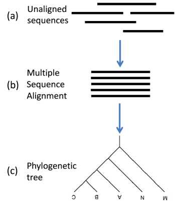
When developing complex algorithms or pipelines in which two or more prediction methods are involved, the uncertainty described in this review should be handled carefully, especially for the intermediate prediction method(s) in the pipeline. For example, let us consider the following pipeline, which is based on two prediction methods (with the example of phylogenetic tree estimation from unaligned sequences in parentheses; see Figure 11):

1. Obtain data $D$ (e.g., $D$ is a set of unaligned sequences $S$).

2. Predict an intermediate solution $\theta^{\prime}\in Y^{\prime}$ from $D$ (e.g., predict a multiple sequence alignment (MSA) $A$ of $S$).

3. Predict the final solution $\theta\in Y$, based on $\theta^{\prime}$ (e.g., predict a phylogenetic tree $T$ based on the multiple alignment $A$)

Given the uncertainty of the intermediate estimation problem (in step 2 above), predicting a single solution $\theta^{\prime}$ should be avoided because point estimation is unreliable. Actually, as discussed in Section 1, the prediction of phylogenetic trees is greatly affected by the uncertainty of multiple alignments [15]. To handle the uncertainty, it is ideal to consider a joint distribution $p(\theta,\theta^{\prime}|D)$ on $Y\times Y^{\prime}$. For instance, $p(\theta,\theta^{\prime}|D)$ could be a joint distribution for a multiple sequence alignment (MSA) and a phylogenetic tree. Then the distribution is marginalized onto $Y$:

$$p(\theta|D)=\sum_{\theta^{\prime}\in Y^{\prime}}p(\theta,\theta^{\prime}|D)\;.$$ (13)

This marginal distribution includes the uncertainty of the intermediate solution $y^{\prime}$. From this marginal distribution, we can predict either one final solution, by using, for example, ML/MEA/MEG estimators (Section 3), or several solutions (see Section 2). However, considering joint distributions (such as Eq. (13)) often leads to huge computational cost, and an approximation could be useful to obtain efficient estimators as shown in the following examples.

Figure 11: A standard method to estimate a phylogenetic tree (topology) from a set of unaligned sequences, in which (b) a multiple sequence alignment (MSA) of sequences is predicted by using a multiple-aligner such as ClustalW or MAFFT [68], and then (c) a phylogenetic tree is predicted from the MSA. Point estimation of an MSA (i.e., step (b)) influences uncertainty and should be avoided if possible.

4.2 Example: Prediction of RNA secondary structure by employing homologous sequence information

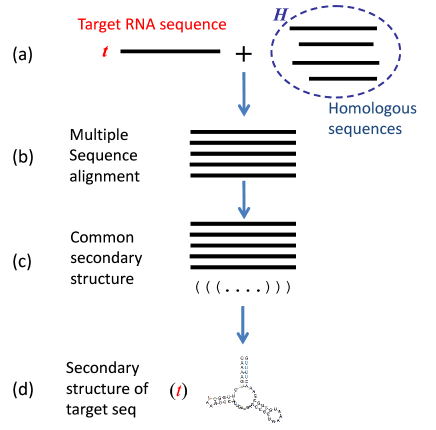
In this section, we consider the problem of predicting an RNA secondary structure by combining homologous sequence information, where the input is the target RNA sequence $t$ and a set of its homologous sequences $H$ (see Figure 12). In this problem, we assume that the target sequence $t$ and each sequence in $H$ share a consensus structure, so the information from the homologous sequences would improve the accuracy of the RNA secondary structure prediction of the target sequence.

One approach to this problem is the following (Figure 12).

1. A multiple sequence alignment for input RNA sequences (both target and homologous sequences) is computed by utilizing a multiple aligner for RNA sequences (such as CentroidAlign [70], Locarna [71] and MAFFT [68]).

2. A common/consensus secondary structure for the multiple alignment is computed by using, e.g., CentroidAlifold [72] and RNAalifold [73].

3. The secondary structure of the target RNA sequence is computed from the predicted common secondary structure by mapping the common structure to the target RNA sequence.

Note that intermediate point estimations are employed twice (in steps 1 and 2) in the above procedure. The results will be affected by the uncertainty of these point estimations, which should therefore be avoided (Section 4.1).

There is a probabilistic model for structural alignments of RNA sequences (known as the Sankoff model [74]), in which both consensus secondary structure and conventional alignments are considered simultaneously. As an alternative to point estimation, it is better to obtain a distribution of RNA secondary structures of the target sequence $t$ by marginalizing (and averaging) the distribution of structural alignments, and then predict a secondary structure for the target by using MEG/MEA estimators or the ML estimator with respect to the marginal probability distribution. However, this approach entails huge computational cost for prediction ($O(L^{6})$ where $L$ is the length of RNA sequences). Hamada et al. [75] approximate this approach by factorizing the distribution of structural alignments into a distribution of secondary structures and a distribution of usual alignments. Furthermore, they showed that the approach in Figure 12 (in which the uncertainty of secondary structures and alignments is not considered) was consistently worse than their method in which the uncertainty of alignments and secondary structures is considered. See [75] for the details.

A similar type of technique was utilized for sequence alignments of RNA sequences [70]. Moreover, a more general form of estimator was introduced in [56].

Figure 12: RNA secondary structure prediction using homologous sequence information. A typical method used to solve this problem is shown, in which two (intermediate) point estimations are made. (a) The input is a target RNA sequence $t$ (whose secondary structure is to be predicted) and a set of homologous sequences $H$. The output is an RNA secondary structure for the target sequence. In the problem, we assume that the target sequence $t$ and each sequence in $H$ share a consensus structure. In the conventional method, (b) a multiple sequence alignment of the target and homologous sequences is predicted; then (c) a common (consensus) secondary structure of the MSA is predicted; finally, (d) the secondary structure of the target sequence is predicted by using the common secondary structure. A more sophisticated approach avoiding point estimations is described in the main text (Section 4.2).

4.3 Example: Variant detection with NGS technologies

In the following pipeline, I try to detect variants of genomes, using next generation sequencing (NGS) technologies.

1. Determine bases (by “base-calling” [76]) from intensity data produced by sequencers (e.g. Illumina, 454, SOLiD and PacBio RS), and obtain a set of reads (i.e., fragmented short sequences).

2. Map (align) the reads to reference genomes by utilizing, e.g., BWA [77], bowtie [78] or LAST [79].

3. Predict single nucleotide polymorphisms (SNPs) and insertions and deletions (INDELs) from the mapped reads obtained in Step 2, using tools such as SAMtools [80] or VarScan [81].

In this pipeline, several point estimations are employed: Step 1 includes the uncertainty of called bases. By retaining the information about the uncertainty of base-calling, most current sequencers produce reads with quality scores in the FASTQ format [82]. Step 2 includes uncertainty with respect to the locations of mapped reads and the detailed alignment between reads and reference genomes. To the best of my knowledge, there is no method that handles these uncertainties completely, although the approach of probabilistic alignments with quality scores [83] partially handles both uncertainties.

5 Discussion

5.1 Usefulness of marginal probabilities

5.1.1 Analyses using marginal probabilities

Due to the uncertainty of single solutions that has been described in this article, considering an ensemble of solutions is useful in the analysis of biological data in bioinformatics. In particular, marginal probabilities (cf. Section 2.3) are often employed in the analyses, because they take into account information about the entire ensemble of solutions.

• In Adachi et al. [52], the analysis of the base-paring probability matrix of an RNA aptamer (bound to a cytokine) suggested that a stem involved in the aptamer was unstable and there was a possibility that it could form several different structures. This was confirmed by biochemical experiments (see Figure 13). It should be emphasized that we could not have obtained this conclusion if only a single predicted structure (e.g., MFE structure) had been considered.

  

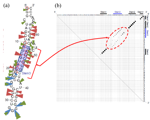
  Figure 13: RNase probing analysis of AptAF42dope1. (a) Fluorescent images of the cleavage products of 50-FAM labeled aptamer with RNase T1, S1 nuclease and RNase V1. (b) Secondary structure of an RNA aptamer predicted by CentroidFold [38], and a base-pairing probability matrix of the aptamer [52]. The base-pairing probabilities in the red circle correspond to an unstable stem. This figure is taken from Figure 4 and Figure 6 in Adachi et al. [52].

• In Halvorsen et al. [84], the authors analyzed the conformation change of RNA secondary structures, cased by a single nucleotide polymorphism (SNP), by utilizing the base-pairing probabilities. They reported seven disease states and phenotypes in which two or more associated SNPs were found to alter the structural ensemble of the RNA (see Table 1 in [84] for the details).

• Iwakiri et al. [85] systematically analyzed base-paring probabilities for paired and unpaired nucleotides of RNA secondary structures involved in known protein-RNA complexes taken from the Protein Data Bank (PDB) [86]. Their analyses lead to novel findings that could not be found if only the snapshots of RNA secondary structures in the PDB are considered.

5.1.2 Algorithms using marginal probabilities: posterior decoding

It should be also remarked that marginal probabilities are employed to construct algorithms, and such an approach is called posterior decoding. Posterior decoding algorithms are widely utilized in bioinformatics: see [53, 87, 88, 83, 13, 89, 90, 91, 92, 93], for example . Actually, most MEG/MEA estimators (Section 3.2) lead to posterior decoding algorithms, because the final algorithm is based on only marginal probabilities. For example, the final algorithm in the $\gamma$-centroid estimators for RNA secondary structure predictions (cf. Section 3.2.3) is based on the base-pairing probability matrix (BPPM) of the RNA sequence (see [58] for the detailed algorithm).

5.2 Uncertainty in hypothesis testing

In several problems in bioinformatics such as homology search [94], a hypothesis testing approach is frequently employed, in which the log odds score of two probabilities relative to a null model is computed instead of the maximum score of the solution. For instance, in homology search, the following (Viterbi) score is utilized:

$$V=\log\frac{\max_{z}p(x,z|H)}{p(x|R)}$$ (14)

where $x$ is a target sequence (we would like to judge whether this sequence is homologous to a query sequence or not), $R$ is a random model (e.g., a one-sate HMM), and $z$ is an alignment between the target and query sequences. The score might be affected by uncertainty because it uses only the maximum score of the optimal alignment. To address this issue, Eddy [95] proposed the use of forward scores,

$$F=\log\frac{\sum_{z}p(x,z|H)}{p(x|R)},$$ (15)

in homology searches of biological sequences. In the forward score, the sum of the probabilities of all solutions (alignments) are utilized, which mitigates the influence of the uncertainty [95].

5.3 Uncertainty introduced by internal parameters in models

In the above, I have focused on the uncertainty of solutions where the probabilistic model (i.e., the probability distribution on the predictive (solution) space) is fixed. On the other hand, a kind of uncertainty also appears with respect to changes of internal parameters in the probabilistic model (e.g., a predicted sequence alignment might be substantially changed by slight changes of the substitution matrix or gap costs in alignments). Several interesting studies have been conducted to address this issue.

In [17, 96, 97], parametric approaches are utilized to enumerate the optimal solutions for all possible changes of internal parameters, which enables the analysis of the parametric behavior of maximum a posteriori (MAP) inference computations. For example, a parametric alignment procedure [98, 97] can efficiently find all the optimal alignments for all possible parameters in a pair Hidden Markov Model (PHMM), which might be one remedy for the uncertainty of solutions introduced by parameter changes. It should be emphasized that the parametric methods can be explained from a unified viewpoint by using a general mathematical theory called tropical geometry [99].

5.4 How to provide probability distributions for solutions

In this review, I have assumed that there exists a probability distribution on a predictive space in the estimation problem (Section 1.3). However, the existence of the probability distribution is not trivial and research on the probability distribution (probabilistic model) for each problem is also important, and much research has been conducted in this area. For example, probabilistic models have been developed for RNA secondary structures [9, 100, 57, 101, 102], alignments [53, 1, 103], gene prediction [63, 104], phylogenetic trees [30] and RNA common secondary structures [73, 72].

5.5 Future directions

By using the approaches described in this review, issues arising from the uncertainty of solutions can be addressed, in part, in several areas of bioinformatics, including RNA secondary structure predictions and sequence alignments. However, it is obvious that uncertainty will raise further serious issues in other fields of bioinformatics. So, in the future, further general methods for fighting against uncertainty, which are applicable to various problems, should be developed: for example, more efficient methods for visualizing or sampling solutions in high-dimensional spaces, methods that mitigate the uncertainly of point estimations, and so forth.

6 Conclusion

In this review, I focused on the uncertainty of solutions (i.e., the fact that the probability of any solution is quite low), which often give rise to serious issues when developing algorithms and analyzing biological data, and introduced several approaches to handle this problem appropriately. I have presented many actual examples in this review and, although most of the examples are related to sequence analyses, such as RNA secondary structure predictions, sequence alignments and phylogenetic tree estimations, I believe that the basic concepts and ideas described in this review will be useful for other problems in many areas of bioinformatics.

Key Points

• Many bioinformatics problems, such as sequence alignment, gene prediction, phylogenetic tree estimation and RNA secondary structure prediction, are often affected by the “uncertainty” of a solution; that is, the probability of the solution is extremely small (e.g., less than $10^{-10}$).

• In the analysis of biological data or the development of prediction algorithms, this uncertainty should be handled carefully and appropriately.

• This review provides several approaches to combat this uncertainty, presenting examples in bioinformatics.

• In particular, point estimations should be handled carefully when designing a pipeline.

• The basic concepts and ideas described in this review will be useful in various areas of bioinformatics.

Biographical note

M.H. is an associate professor at Department of Computational Biology, the University of Tokyo. His background is pure mathematics and his research interests include any mathematical aspects of bioinformatics.

Supplementary Information

The IDs of references correspond to those of the main manuscript in the following.

Appendix A How to compute suboptimal solutions in Mfold

In this appendix, I briefly introduce an algorithm that predicts suboptimal RNA secondary structures, which is described in Zuker [19].

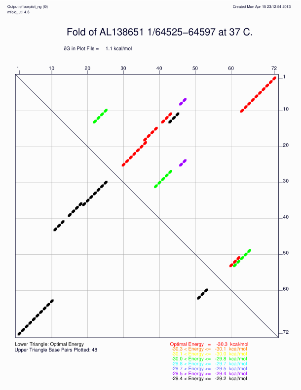
Let $\Delta G$ be the minimum free energy (MFE) of secondary structures of a given RNA sequence, and let $\Delta G(i,j)$ be the minimum free energy of secondary structures that contain the $(i,j)$ base-pair. Then, the energy dot plot (Figure S1) is defined as a set of base-pairs as follows:

$$\mathcal{P}=\{(i,j)|\Delta G(i,j)\leq\Delta G+\varepsilon\}$$

where $\varepsilon$ is equal to $\Delta G\times\frac{p}{100}$. Then, Mfold computes a set of suboptimal secondary structures (denoted by $\mathcal{S}$) as follows:

1. $\mathcal{S}$ is set to $\emptyset$.

2. $L$ is a list of base-pairs in $\mathcal{P}$, which is sorted in order of increasing $\Delta G(i,j)$.

3. The base-pair $(i,j)$ at the top of list $L$ is selected.

4. Predict the secondary structure $s$, with minimum free energy, that contains the base-pair $(i,j)$.

5. If $s$ contains at least $W$ base pairs that were not found in previous foldings (in $\mathcal{S}$) then make the replacement $\mathcal{S}\leftarrow\mathcal{S}\cup\{s\}$ and remove the base-pairs of $s$ from the list $L$.

6. Go to Step 2 and repeat the procedure until the maximum number of suboptimal secondary structures (specified by a user) is reached or no base-pair is found in $L$.

Figure S1: (Upper right) An energy dot plot for a tRNA sequence (AL138651.1/64525–64597), produced by Mfold Web Server (http://mfold.rna.albany.edu/?q=mfold) [20]. Base-pairs with warmer colors have lower free energy, compared to the ones with colder colors. (Lower left) The secondary structure of the MFE structure.

Appendix B Evaluation measures in RNA secondary structure predictions

The evaluation of a predicted RNA secondary structure is usually based on base-pairs. First, we define

$$TP=\sum_{i<j}I(y_{ij}=1)I(\theta_{ij}=1),\ TN=\sum_{i<j}I(y_{ij}=0)I(\theta_{ij}=0)$$

$$FP=\sum_{i<j}I(y_{ij}=1)I(\theta_{ij}=0),\ FN=\sum_{i<j}I(y_{ij}=0)I(\theta_{ij}=1)$$

for a reference secondary structure $\theta$ and a predicted structure $y$; $I(\cdot)$ is the indicator function, which takes a value of 1 or 0 depending on whether the condition constituting its argument is true or false. These four parameters count the numbers of true positives (TP), true negatives (TN), false positives (FP) and false negatives (FN). From these we can construct three accuracy measures that can be used for evaluation: the sensitivity (SEN), positive predictive value (PPV) and the Matthew Correlation Coefficient (MCC).

$$\mbox{SEN}=\frac{\mbox{TP}}{\mbox{TP}+\mbox{FN}}$$ (S1)

$$\mbox{PPV}=\frac{\mbox{TP}}{\mbox{TP}+\mbox{FP}}$$ (S2)

$$\mbox{MCC}={\small\frac{\mbox{TP}\cdot\mbox{TN}-\mbox{FP}\cdot\mbox{FN}}{\sqrt{(\mbox{TP}+\mbox{FP})(\mbox{TP}+\mbox{FN})(\mbox{TN}+\mbox{FP})(\mbox{TN}+\mbox{FN})}}}.$$ (S3)

There is a tradeoff between SEN and PPV, while MCC is an accuracy measure which balances those two measures.

Appendix C Generalized estimators of Section 3.2.4

The approximate estimator described in Section 3.2.4 can be adapted to utilize more general accuracy measures as follows.

$$\hat{y}=\mathop{\mathrm{arg\ max}}_{y\in\mathcal{S}(x)}\sum_{\theta\in\mathcal{S}(x)}Acc(\theta,y)p(\theta|x)$$ (S4)

where $Acc$ is a function of TP, TN, FP and FN (including MCC and F-score):

$$Acc=f(\mbox{TP},\mbox{TN},\mbox{FP},\mbox{FN}).$$

For this general accuracy measure, let us define the pseudo-expected accuracy by

$$\widehat{Acc}^{0}(y)=f(\widehat{\mbox{TP}},\widehat{\mbox{TN}},\widehat{\mbox{FP}},\widehat{\mbox{FN}}).$$ (S5)

Finally, the estimator

$$\hat{y}=\mathop{\mathrm{argmax}}_{y\in\mathcal{S}(x)}\widehat{Acc}^{0}(y).$$ (S6)

is obtained, and the computation is conducted in combination with stochastic sampling (Section 2.1.1).

Appendix D Supplementary Figure

Figure S2: Visualization of RNA base-pairing probabilities by RNABow [51].

References

- [1] Durbin R, Eddy S, Krogh A, et al. Biological Sequence Analysis: Probabilistic Models of Proteins and Nucleic Acids. Cambridge University Press, 1998.
- [2] Yandell M, Ence D. A beginner’s guide to eukaryotic genome annotation. Nat. Rev. Genet., 13(5):329–342, May 2012.
- [3] Seetin MG, Mathews DH. RNA structure prediction: an overview of methods. Methods Mol. Biol., 905:99–122, 2012.
- [4] Aigner K, Dreßen F, Steger G. Methods for predicting rna secondary structure. In Leontis N, Westhof E, editors, RNA 3D Structure Analysis and Prediction, volume 27 of Nucleic Acids and Molecular Biology, pages 19–41. Springer Berlin Heidelberg, 2012.
- [5] Kato Y, Sato K, Hamada M, et al. RactIP: fast and accurate prediction of RNA-RNA interaction using integer programming. Bioinformatics, 26(18):i460–466, Sep 2010.
- [6] Yang Z. Computational Molecular Evolution. Oxford University Press, Oxford, 2006.
- [7] Proctor JR, Meyer IM. COFOLD: an RNA secondary structure prediction method that takes co-transcriptional folding into account. Nucleic Acids Res., 41(9):e102, May 2013.
- [8] Hofacker IL, Priwitzer B, Stadler PF. Prediction of locally stable RNA secondary structures for genome-wide surveys. Bioinformatics, 20(2):186–190, Jan 2004.
- [9] McCaskill JS. The equilibrium partition function and base pair binding probabilities for RNA secondary structure. Biopolymers, 29(6-7):1105–1119, 1990.
- [10] Barash D, Churkin A. Mutational analysis in RNAs: comparing programs for RNA deleterious mutation prediction. Brief. Bioinformatics, 12(2):104–114, Mar 2011.
- [11] Churkin A, Barash D. RNAmute: RNA secondary structure mutation analysis tool. BMC Bioinformatics, 7:221, 2006.
- [12] Waldispuhl J, Devadas S, Berger B, et al. Efficient algorithms for probing the RNA mutation landscape. PLoS Comput. Biol., 4(8):e1000124, 2008.
- [13] Lunter G, Rocco A, Mimouni N, et al. Uncertainty in homology inferences: assessing and improving genomic sequence alignment. Genome Res., 18(2):298–309, Feb 2008.
- [14] Manzourolajdad A, Wang Y, Shaw TI, et al. Information-theoretic uncertainty of SCFG-modeled folding space of the non-coding RNA. J. Theor. Biol., 318C:140–163, Nov 2012.
- [15] Wong KM, Suchard MA, Huelsenbeck JP. Alignment uncertainty and genomic analysis. Science, 319(5862):473–476, Jan 2008.
- [16] Fletcher W, Yang Z. The effect of insertions, deletions, and alignment errors on the branch-site test of positive selection. Mol. Biol. Evol., 27(10):2257–2267, Oct 2010.
- [17] Malaspinas AS, Eriksson N, Huggins P. Parametric analysis of alignment and phylogenetic uncertainty. Bull. Math. Biol., 73(4):795–810, Apr 2011.
- [18] Waterman MS. Introduction to Computational Biology: Maps, Sequences and Genomes. Chapman & Hall, London, 1995.
- [19] Zuker M. On finding all suboptimal foldings of an RNA molecule. Science, 244(4900):48–52, Apr 1989.
- [20] Zuker M. Mfold web server for nucleic acid folding and hybridization prediction. Nucleic Acids Res., 31(13):3406–3415, Jul 2003.
- [21] Ding Y, Lawrence CE. A bayesian statistical algorithm for RNA secondary structure prediction. Comput. Chem., 23(3-4):387–400, Jun 1999.
- [22] Wuchty S, Fontana W, Hofacker IL, et al. Complete suboptimal folding of RNA and the stability of secondary structures. Biopolymers, 49(2):145–165, Feb 1999.
- [23] Geyer CJ. Practical Markov Chain Monte Carlo. Statistical Science, 7(4):473–483, 1992.
- [24] Meyer IM, Miklos I. SimulFold: simultaneously inferring RNA structures including pseudoknots, alignments, and trees using a Bayesian MCMC framework. PLoS Comput. Biol., 3(8):e149, Aug 2007.
- [25] Metzler D, Nebel ME. Predicting RNA secondary structures with pseudoknots by MCMC sampling. J Math Biol, 56(1-2):161–181, Jan 2008.
- [26] Bon M, Micheletti C, Orland H. McGenus: a Monte Carlo algorithm to predict RNA secondary structures with pseudoknots. Nucleic Acids Res., 41(3):1895–1900, Feb 2013.
- [27] Saule C, Regnier M, Steyaert JM, et al. Counting RNA pseudoknotted structures. J. Comput. Biol., 18(10):1339–1351, Oct 2011.
- [28] Doose G, Metzler D. Bayesian sampling of evolutionarily conserved RNA secondary structures with pseudoknots. Bioinformatics, 28(17):2242–2248, Sep 2012.
- [29] Wei D, Alpert LV, Lawrence CE. RNAG: a new Gibbs sampler for predicting RNA secondary structure for unaligned sequences. Bioinformatics, 27(18):2486–2493, Sep 2011.
- [30] Huelsenbeck JP, Ronquist F. MRBAYES: Bayesian inference of phylogenetic trees. Bioinformatics, 17(8):754–755, Aug 2001.
- [31] Satija R, Novak A, Miklos I, et al. BigFoot: Bayesian alignment and phylogenetic footprinting with MCMC. BMC Evol. Biol., 9:217, 2009.
- [32] Clote P. An efficient algorithm to compute the landscape of locally optimal RNA secondary structures with respect to the Nussinov-Jacobson energy model. J. Comput. Biol., 12(1):83–101, 2005.
- [33] Saffarian A, Giraud M, Monte de A, et al. RNA locally optimal secondary structures. J. Comput. Biol., 19(10):1120–1133, Oct 2012.
- [34] Steffen P, Voss B, Rehmsmeier M, et al. RNAshapes: an integrated RNA analysis package based on abstract shapes. Bioinformatics, 22(4):500–503, Feb 2006.
- [35] Giegerich R, Meyer C. Algebraic dynamic programming. In Algebraic Methodology And Software Technology, 9th International Conference, AMAST 2002, pages 349–364. Springer LNCS, 2002.
- [36] Voss B, Giegerich R, Rehmsmeier M. Complete probabilistic analysis of RNA shapes. BMC Biol., 4:5, 2006.
- [37] Ding Y, Chan CY, Lawrence CE. RNA secondary structure prediction by centroids in a Boltzmann weighted ensemble. RNA, 11(8):1157–1166, Aug 2005.
- [38] Sato K, Hamada M, Asai K, et al. CENTROIDFOLD: a web server for RNA secondary structure prediction. Nucleic Acids Res., 37(Web Server issue):W277–280, Jul 2009.
- [39] Kruskal JB, Wish M. Multidimensional Scaling. Sage Publications, 275 South Beverly Drive, Beverly Hills, CA 90212, 1978.
- [40] Amenta N, Klingner J. Case study: visualizing sets of evolutionary trees. In Information Visualization, 2002. INFOVIS 2002. IEEE Symposium on, pages 71–74, 2002.
- [41] Hillis DM, Heath TA, St John K. Analysis and visualization of tree space. Syst. Biol., 54(3):471–482, Jun 2005.
- [42] Robinson D, Foulds L. Comparison of phylogenetic trees. Mathematical Biosciences, 53(1–2):131–147, 1981.
- [43] Huang H, Li Y. MASTtreedist: visualization of tree space based on maximum agreement subtree. J. Comput. Biol., 20(1):42–49, Jan 2013.
- [44] David Bryant. Building Trees, Hunting for Trees, and Comparing Trees - Theory and Methods in Phylogenetic Analysis, 1997. Ph.D. dissertation, University of Canterbury, Christchurch, New Zealand.
- [45] Newberg LA, Lawrence CE. Exact calculation of distributions on integers, with application to sequence alignment. J. Comput. Biol., 16(1):1–18, Jan 2009.
- [46] Freyhult E, Moulton V, Clote P. RNAbor: a web server for RNA structural neighbors. Nucleic Acids Res., 35(Web Server issue):W305–309, Jul 2007.
- [47] Freyhult E, Moulton V, Clote P. Boltzmann probability of RNA structural neighbors and riboswitch detection. Bioinformatics, 23(16):2054–2062, Aug 2007.
- [48] Clote P, Lou F, Lorenz WA. Maximum expected accuracy structural neighbors of an RNA secondary structure. BMC Bioinformatics, 13 Suppl 5:S6, 2012.
- [49] Lorenz R, Flamm C, Hofacker IL. 2d projections of rna folding landscapes. In Grosse I, Neumann S, Posch S, et al., editors, GCB, volume 157 of LNI, pages 11–20. GI, 2009.
- [50] Burge SW, Daub J, Eberhardt R, et al. Rfam 11.0: 10 years of RNA families. Nucleic Acids Res., 41(Database issue):D226–232, Jan 2013.
- [51] Aalberts DP, Jannen WK. Visualizing RNA base-pairing probabilities with RNAbow diagrams. RNA, Feb 2013.
- [52] Adachi H, Ishiguro A, Hamada M, et al. Antagonistic RNA aptamer specific to a heterodimeric form of human interleukin-17A/F. Biochimie, 93(7):1081–1088, Jul 2011.
- [53] Miyazawa S. A reliable sequence alignment method based on probabilities of residue correspondences. Protein Eng., 8(10):999–1009, Oct 1995.
- [54] Iwasaki W, Takagi T. An intuitive, informative, and most balanced representation of phylogenetic topologies. Syst. Biol., 59(5):584–593, Oct 2010.
- [55] Carvalho LE, Lawrence CE. Centroid estimation in discrete high-dimensional spaces with applications in biology. Proc. Natl. Acad. Sci. U.S.A., 105(9):3209–3214, Mar 2008.
- [56] Hamada M, Kiryu H, Iwasaki W, et al. Generalized centroid estimators in bioinformatics. PLoS ONE, 6(2):e16450, 2011.
- [57] Do CB, Woods DA, Batzoglou S. CONTRAfold: RNA secondary structure prediction without physics-based models. Bioinformatics, 22(14):e90–98, Jul 2006.
- [58] Hamada M, Kiryu H, Sato K, et al. Prediction of RNA secondary structure using generalized centroid estimators. Bioinformatics, 25(4):465–473, Feb 2009.
- [59] Hamada M, Asai K. A classification of bioinformatics algorithms from the viewpoint of maximizing expected accuracy (MEA). J. Comput. Biol., 19(5):532–549, May 2012.
- [60] Hamada M, Sato K, Asai K. Prediction of RNA secondary structure by maximizing pseudo-expected accuracy. BMC Bioinformatics, 11:586, 2010.
- [61] Frith MC, Hamada M, Horton P. Parameters for accurate genome alignment. BMC Bioinformatics, 11:80, 2010.
- [62] Zhang MQ. Computational prediction of eukaryotic protein-coding genes. Nat. Rev. Genet., 3(9):698–709, Sep 2002.
- [63] Gross SS, Do CB, Sirota M, et al. CONTRAST: a discriminative, phylogeny-free approach to multiple informant de novo gene prediction. Genome Biol., 8(12):R269, 2007.
- [64] Lorenz R, Bernhart SH, Honer Zu Siederdissen C, et al. ViennaRNA Package 2.0. Algorithms Mol Biol, 6:26, 2011.
- [65] Bradley RK, Roberts A, Smoot M, et al. Fast statistical alignment. PLoS Comput. Biol., 5(5):e1000392, May 2009.
- [66] Kim J, Ma J. PSAR: measuring multiple sequence alignment reliability by probabilistic sampling. Nucleic Acids Res., 39(15):6359–6368, Aug 2011.
- [67] Webb-Robertson BJ, McCue LA, Lawrence CE. Measuring global credibility with application to local sequence alignment. PLoS Comput. Biol., 4(5):e1000077, May 2008.
- [68] Katoh K, Standley DM. MAFFT Multiple Sequence Alignment Software Version 7: Improvements in Performance and Usability. Mol. Biol. Evol., Feb 2013.
- [69] Eddy SR, Durbin R. RNA sequence analysis using covariance models. Nucleic Acids Res., 22(11):2079–2088, Jun 1994.
- [70] Hamada M, Sato K, Kiryu H, et al. CentroidAlign: fast and accurate aligner for structured RNAs by maximizing expected sum-of-pairs score. Bioinformatics, 25(24):3236–3243, Dec 2009.
- [71] Will S, Reiche K, Hofacker IL, et al. Inferring noncoding RNA families and classes by means of genome-scale structure-based clustering. PLoS Comput. Biol., 3(4):e65, Apr 2007.
- [72] Hamada M, Sato K, Asai K. Improving the accuracy of predicting secondary structure for aligned RNA sequences. Nucleic Acids Res., 39(2):393–402, Jan 2011.
- [73] Bernhart SH, Hofacker IL, Will S, et al. RNAalifold: improved consensus structure prediction for RNA alignments. BMC Bioinformatics, 9:474, 2008.
- [74] Sankoff D. Simultaneous solution of the RNA folding alignment and protosequence problems. SIAM J. Appl. Math, pages 810–825, 1985.
- [75] Hamada M, Sato K, Kiryu H, et al. Predictions of RNA secondary structure by combining homologous sequence information. Bioinformatics, 25(12):i330–338, Jun 2009.
- [76] Ledergerber C, Dessimoz C. Base-calling for next-generation sequencing platforms. Brief. Bioinformatics, 12(5):489–497, Sep 2011.
- [77] Li H, Durbin R. Fast and accurate short read alignment with Burrows-Wheeler transform. Bioinformatics, 25(14):1754–1760, Jul 2009.
- [78] Langmead B, Salzberg SL. Fast gapped-read alignment with Bowtie 2. Nat. Methods, 9(4):357–359, Apr 2012.
- [79] Shrestha AM, Frith MC. An approximate Bayesian approach for mapping paired-end DNA reads to a reference genome. Bioinformatics, 29(8):965–972, Apr 2013.
- [80] Li H, Handsaker B, Wysoker A, et al. The Sequence Alignment/Map format and SAMtools. Bioinformatics, 25(16):2078–2079, Aug 2009.
- [81] Koboldt DC, Zhang Q, Larson DE, et al. VarScan 2: somatic mutation and copy number alteration discovery in cancer by exome sequencing. Genome Res., 22(3):568–576, Mar 2012.
- [82] Cock PJ, Fields CJ, Goto N, et al. The Sanger FASTQ file format for sequences with quality scores, and the Solexa/Illumina FASTQ variants. Nucleic Acids Res., 38(6):1767–1771, Apr 2010.
- [83] Hamada M, Wijaya E, Frith MC, et al. Probabilistic alignments with quality scores: an application to short-read mapping toward accurate SNP/indel detection. Bioinformatics, 27(22):3085–3092, Nov 2011.
- [84] Halvorsen M, Martin JS, Broadaway S, et al. Disease-associated mutations that alter the RNA structural ensemble. PLoS Genet., 6(8):e1001074, Aug 2010.
- [85] Iwakiri J, Kameda T, Asai K, et al. Analysis of base-pairing probabilities of RNA molecules involved in protein-RNA interactions, 2013. (submitted).
- [86] Berman HM, Westbrook J, Feng Z, et al. The Protein Data Bank. Nucleic Acids Res., 28(1):235–242, Jan 2000.
- [87] Holmes I, Durbin R. Dynamic programming alignment accuracy. J. Comput. Biol., 5(3):493–504, 1998.
- [88] Knudsen B, Hein J. RNA secondary structure prediction using stochastic context-free grammars and evolutionary history. Bioinformatics, 15(6):446–454, Jun 1999.
- [89] Fariselli P, Martelli PL, Casadio R. A new decoding algorithm for hidden Markov models improves the prediction of the topology of all-beta membrane proteins. BMC Bioinformatics, 6 Suppl 4:S12, Dec 2005.
- [90] Phuong TM, Do CB, Edgar RC, et al. Multiple alignment of protein sequences with repeats and rearrangements. Nucleic Acids Res., 34(20):5932–5942, 2006.
- [91] Liu Y, Schmidt B, Maskell DL. MSAProbs: multiple sequence alignment based on pair hidden Markov models and partition function posterior probabilities. Bioinformatics, 26(16):1958–1964, Aug 2010.
- [92] Wilm A, Higgins DG, Notredame C. R-Coffee: a method for multiple alignment of non-coding RNA. Nucleic Acids Res., 36(9):e52, May 2008.
- [93] Lunter G, Miklos I, Drummond A, et al. Bayesian coestimation of phylogeny and sequence alignment. BMC Bioinformatics, 6:83, 2005.
- [94] Eddy SR. A new generation of homology search tools based on probabilistic inference. Genome Inform, 23(1):205–211, Oct 2009.
- [95] Eddy SR. A probabilistic model of local sequence alignment that simplifies statistical significance estimation. PLoS Comput. Biol., 4(5):e1000069, May 2008.
- [96] Pachter L, Sturmfels B. Parametric inference for biological sequence analysis. Proc. Natl. Acad. Sci. U.S.A., 101(46):16138–16143, Nov 2004.
- [97] Dewey CN, Huggins PM, Woods K, et al. Parametric alignment of Drosophila genomes. PLoS Comput. Biol., 2(6):e73, Jun 2006.
- [98] Waterman MS, Eggert M, Lander E. Parametric sequence comparisons. Proceedings of the National Academy of Sciences of the United States of America, 89(13):6090–6093, July 1992.
- [99] Pachter L, Sturmfels B. Tropical geometry of statistical models. Proc. Natl. Acad. Sci. U.S.A., 101(46):16132–16137, Nov 2004.
- [100] Andronescu M, Condon A, Hoos HH, et al. Computational approaches for RNA energy parameter estimation. RNA, 16(12):2304–2318, Dec 2010.
- [101] Sato K, Hamada M, Mituyama T, et al. A non-parametric bayesian approach for predicting rna secondary structures. J. Bioinformatics and Computational Biology, 8(4):727–742, 2010.
- [102] Rivas E, Lang R, Eddy SR. A range of complex probabilistic models for RNA secondary structure prediction that includes the nearest-neighbor model and more. RNA, 18(2):193–212, Feb 2012.
- [103] Do C, Gross S, Batzoglou S. CONTRAlign: Discriminative training for protein sequence alignment. 2006.
- [104] Pedersen JS, Hein J. Gene finding with a hidden Markov model of genome structure and evolution. Bioinformatics, 19(2):219–227, Jan 2003.