Excitation spectrum of interacting Bosons
in the mean-field infinite-volume limit

Abstract.

We consider homogeneous Bose gas in a large cubic box with periodic boundary conditions, at zero temperature. We analyze its excitation spectrum in a certain kind of a mean field infinite volume limit. We prove that under appropriate conditions the excitation spectrum has the form predicted by the Bogoliubov approximation. Our result can be viewed as an extension of the result of Seiringer [18] to large volumes.

1. Introduction and main results

Many physical properties of complicated interacting systems can be derived from simple Hamiltonians invoving independent (bosonic or fermionic) quasiparticles (see [5] for a detailed discussion of this concept) with appropriately chosen dispersion relation (the dependence of the quasiparticle energy on the momentum). One of such systems is the weakly interacting Bose gas at zero temperature. On the heuristic level, the quasiparticle description of the Bose gas can be derived from the Bogoliubov approximation ([2], see also [4]). The main goal of this paper is a rigorous justification of this approximation for a homogeneous system of $N$ interacting bosons in a certain kind of a mean field large volume limit.

Let us state the assumptions on the 2-body potential that we will use throughout the paper. Consider a real function $\mathbb{R}^{d}\ni\mathbf{x}\mapsto v(\mathbf{x})$, with its Fourier transform defined by

$$\hat{v}(\mathbf{p}):=\int_{\mathbb{R}^{d}}v(\mathbf{x})\operatorname{e}^{-{\operatorname{i}}\mathbf{p}\mathbf{x}}{\operatorname{d}}\mathbf{x}.$$

We assume that $v(\mathbf{x})=v(-\mathbf{x})$, and that $v\in L^{1}(\mathbb{R}^{d})$ and $\hat{v}\in L^{1}(\mathbb{R}^{d})$. We also suppose that the potential is positive and positive definite, i.e.

$$v(\mathbf{x})\geq 0,\ \ \mathbf{x}\in\mathbb{R}^{d},\ \ \ \ \hat{v}(\mathbf{p})\geq 0,\,\,\,\mathbf{p}\in\mathbb{R}^{d}.$$

We will consider Bose gas in large but finite volume. To do this, following the standard approach, we replace the infinite space ${\mathbb{R}}^{d}$ by the torus $\Lambda=]-L/2,L/2]^{d}$, that is, the $d$-dimensional cubic box of side length $L$. We will always assume that $L\geq 1$.

The original potential $v$ is replaced by its periodized version

$$v^{L}(\mathbf{x}):=\frac{1}{L^{d}}\sum_{\mathbf{p}\in(2\pi/L)\mathbb{Z}^{d}}\operatorname{e}^{{\operatorname{i}}\mathbf{p}\mathbf{x}}\hat{v}(\mathbf{p}).$$

Here, $\mathbf{p}\in(2\pi/L)\mathbb{Z}^{d}$ is the discrete momentum variable. Note that $v^{L}$ is periodic with respect to the domain $\Lambda$ and that $v^{L}(\mathbf{x})\rightarrow v(\mathbf{x})$ as $L\to\infty$. Consider the Hamiltonian

$$-\sum_{i=1}^{N}\Delta^{L}_{i}+\lambda\sum_{1\leq i<j\leq N}v^{L}(\mathbf{x}_{i}-\mathbf{x}_{j})$$ (1.1)

acting on the space $L^{2}_{{\operatorname{s}}}(\Lambda^{N})$ (the symmetric subspace of $L^{2}(\Lambda^{N})$) The Laplacian is assumed to have periodic boundary conditions.

Let $\rho=N/L^{d}$ be the density of the gas. The Bogoliubov approximation [2] predicts that the ground state energy is

$$\frac{1}{2}\lambda\rho\hat{v}({\mathbf{0}})(N-1)-\frac{1}{2}\sum_{\mathbf{p}\in\frac{2\pi}{L}\mathbb{Z}^{d}\setminus\{0\}}\left(|\mathbf{p}|^{2}+\rho\lambda\hat{v}(\mathbf{p})-|\mathbf{p}|\sqrt{|\mathbf{p}|^{2}+2\rho\lambda\hat{v}(\mathbf{p})}\right)$$

and that the low lying excited states can be derived from the following elementary excitation spectrum:

$$|\mathbf{p}|\sqrt{|\mathbf{p}|^{2}+2\rho\lambda\hat{v}(\mathbf{p})}.$$ (1.2)

Note that within the Bogoliubov approximation both the ground state energy and the excitation spectrum depend on $\rho$ and $\lambda$ only through the product $\rho\lambda$. The dependence on $L$ is very weak:

1. The elementary excitation spectrum (1.2) depends on $L$ only through the spacing of the momentum lattice $\frac{2\pi}{L}{\mathbb{Z}}^{d}$.

2. The expression for the ground state energy divided by the volume $L^{d}$ converges for $L\to\infty$ to a finite expression

   $$\frac{1}{2}\rho^{2}\lambda\hat{v}({\mathbf{0}})-\frac{1}{2(2\pi)^{d}}\int\left(|\mathbf{p}|^{2}+\rho\lambda\hat{v}(\mathbf{p})-|\mathbf{p}|\sqrt{|\mathbf{p}|^{2}+2\rho\lambda\hat{v}(\mathbf{p})}\right){\operatorname{d}}\mathbf{p}.$$ (1.3)

We believe that it is important to understand the Bogoliubov approximation for large $L$. Important physical properties, such as the phonon group velocity and the description of the Beliaev damping in terms of analyticity properties of Green’s functions, have an elegant description when we can view the momentum as a continuous variable, which is equivalent to taking the limit $L\to\infty$.

Note that in our problem there are three a priori uncorrelated parameters: $\lambda$, $N$ and $L$. By the mean field limit one usually understands $N\to\infty$ with $\lambda\simeq\frac{1}{N}$ and $L=\rm{const.}$ However, when both $N$ and $L$ are large it is natural to consider a somewhat different scaling. In our paper the mean field limit will correspond to $N\to\infty$ with $\lambda\simeq\frac{1}{\rho}=\frac{L^{d}}{N}$.

Motivated by the above argument we will consider a system described by the Hamiltonian

$$H_{N}^{L}=-\sum_{i=1}^{N}\Delta^{L}_{i}+\frac{L^{d}}{N}\sum_{1\leq i<j\leq N}v^{L}(\mathbf{x}_{i}-\mathbf{x}_{j}).$$ (1.4)

It is translation invariant – it commutes with the total momentum operator

$$P_{N}^{L}:=-\sum_{i=1}^{N}{\operatorname{i}}\partial_{\mathbf{x}_{i}}^{L}.$$ (1.5)

We will denote by $E_{N}^{L}$ the ground state energy of (1.4). If $\mathbf{p}\in\frac{2\pi}{L}{\mathbb{Z}}^{d}\backslash\{{\mathbf{0}}\}$ let $K_{N}^{L,1}(\mathbf{p}),K_{N}^{L,2}(\mathbf{p}),\dots$ be the eigenvalues of $H_{N}^{L}-E_{N}^{L}$ of total momentum $\mathbf{p}$ in the order of increasing values, counting the multiplicity. The lowest eigenvalue of $H_{N}^{L}-E_{N}^{L}$ of total momentum $\mathbf{p}={\mathbf{0}}$ is $0$ by general arguments [4]. Let $K_{N}^{L,1}({\mathbf{0}}),K_{N}^{L,2}({\mathbf{0}}),\dots$ be the next eigenvalues of $H_{N}^{L}-E_{N}^{L}$ of total momentum ${\mathbf{0}}$, also in the order of increasing values, counting the multiplicity.

We also introduce the Bogoliubov energy

$$E_{\operatorname{Bog}}^{L}:=-\frac{1}{2}\sum_{\mathbf{p}\in\frac{2\pi}{L}\mathbb{Z}^{d}\setminus\{0\}}\left(|\mathbf{p}|^{2}+\hat{v}(\mathbf{p})-|\mathbf{p}|\sqrt{|\mathbf{p}|^{2}+2\hat{v}(\mathbf{p})}\right)$$

and the Bogoliubov elementary excitation spectrum

$$e_{\mathbf{p}}=|\mathbf{p}|\sqrt{|\mathbf{p}|^{2}+2\hat{v}(\mathbf{p})}.$$ (1.6)

For any $\mathbf{p}\in\frac{2\pi}{L}{\mathbb{Z}}^{d}$ we consider the corresponding excitation energies with momentum $\mathbf{p}$:

$$\Big{\{}\sum_{i=1}^{j}e_{{\bf k}_{i}}\ :\ {\bf k}_{1},\dots,{\bf k}_{j}\in\frac{2\pi}{L}{\mathbb{Z}}^{d}\backslash\{{\mathbf{0}}\},\ {\bf k}_{1}+\cdots+{\bf k}_{j}=\mathbf{p},\ \ j=1,2,\dots\Big{\}}.$$

Let $K_{\operatorname{Bog}}^{L,1}(\mathbf{p}),K_{\operatorname{Bog}}^{L,2}(\mathbf{p}),\dots$ be these excitation energies in the order of increasing values, counting the multiplicity. We will use the term excitation spectrum in the Bogoliubov approximation to denote the set of pairs $\big{(}K_{\operatorname{Bog}}^{L,j}(\mathbf{p}),\mathbf{p}\big{)}\in{\mathbb{R}}\times{\mathbb{R}}^{d}$. Later on we will see that it coincides with the joint spectrum of commuting operators $H_{\operatorname{Bog}}^{L}-E^{L}_{\operatorname{Bog}}$ and $P^{L}$ with $(0,{\mathbf{0}})$ removed. (See (6.3) for the definition of $H_{\operatorname{Bog}}^{L}$.)

Below we present pictures of the excitation spectrum of 1-dimensional Bose gas in the Bogoliubov approximation for two potentials, $v_{1}$ and $v_{2}$. Both potentials are appropriately scaled Gaussians. (Note that Gaussians satisfy the assumptions of our main theorem). On both pictures the (black) dot at the origin corresponds to the quasiparticle vacuum, (red) dots correspond to 1-quasiparticle excitations, (blue) triangles correspond to 2-quasiparticles excitations, while (green) squares correspond to $n$-quasiparticles excitations with $n\geq 3$. We also give the graphs of the Fourier transforms of both potentials.

Note that all figures are drawn in the same scale, apart from Fig. 4. where the potential had to be scaled down because of space limitations. In our units of length $\frac{2\pi}{L}=\frac{15}{100}$.

Notice that for some total momentum $\mathbf{p}$ many-quasiparticle excitation energies are lower than the elementary excitation spectrum. In particular, for the potential $v_{1}$ it happens already for low momenta. Physically this means that the corresponding 1-quasiparticle excitation is not stable: it may decay to $m$-quasiparticle states, $m\geq 2$, with a lower energy. This phenomenon has been observed experimentally [10] and is called the Beliaev damping [1]. If one can assume that the momentum variable is continuous, the Beliaev damping corresponds to a pole of the Green’s function on a non-physical sheet of the energy complex plane. The imaginary part of the position of this pole, computed by Beliaev, is responsible for the rate of decay of quasiparticles.

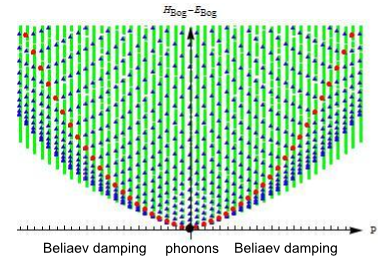
Figure 1. Excitation spectrum of 1-dimensional homogeneous Bose gas with potential $v_{1}$ in the Bogoliubov approximation.

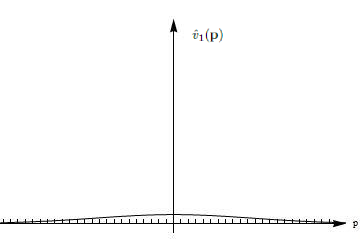
Figure 2. $\hat{v}_{1}(\mathbf{p})=\frac{\operatorname{e}^{-\mathbf{p}^{2}/5}}{10}$.

The excitation spectrum for potential $v_{2}$ has a very different shape – it has local maxima and local minima away from the zero momentum. On the picture we show traditional names of quasiparticles – phonons in the low momentum region, where the dispersion relation is approximately linear, maxons near the local maximum and rotons near the local minimum of the elementary excitation spectrum (see [9] for details).

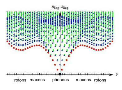
Figure 3. Excitation spectrum of 1-dimensional homogeneous Bose gas with potential $v_{2}$ in the Bogoliubov approximation.

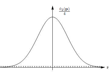
Figure 4. $\hat{v}_{2}(\mathbf{p})=\frac{15\operatorname{e}^{-\mathbf{p}^{2}/2}}{2}$.

From now on, we will drop the superscript $L$. Let us state our main result. It is slightly different for the upper and lower bound:

Theorem 1.1.

1. Let $c>0$. Then there exists $C$ such that

   1. if

      $$L^{2d+2}\leq cN,$$ (1.7)

      then

      $$E_{N}\geq\frac{1}{2}\hat{v}({\mathbf{0}})(N-1)+E_{\operatorname{Bog}}-CN^{-1/2}L^{2d+3};$$ (1.8)

   2. if in addition

      $$K_{N}^{j}(\mathbf{p})\leq cNL^{-d-2},$$ (1.9)

      then

      $$E_{N}+K_{N}^{j}(\mathbf{p}) \geq \frac{1}{2}\hat{v}({\mathbf{0}})(N-1)+E_{\operatorname{Bog}}+K_{\operatorname{Bog}}^{j}(\mathbf{p})$$ (1.10)

      $$-CN^{-1/2}L^{d/2+3}\big{(}K_{N}^{j}(\mathbf{p})+L^{d}\big{)}^{3/2}.$$

2. Let $c>0$. Then there exists $c_{1}>0$ and $C$ such that

   1. if

      $$L^{2d+1} \leq cN$$ (1.11)

      $$\hbox{ and }\hskip 17.22217ptL^{d+1} \leq c_{1}N,$$ (1.12)

      then

      $$E_{N}\leq\frac{1}{2}\hat{v}({\mathbf{0}})(N-1)+E_{\operatorname{Bog}}+CN^{-1/2}L^{2d+3/2};$$ (1.13)

   2. if in addition

      $$K_{\operatorname{Bog}}^{j}(\mathbf{p}) \leq cNL^{-d-2}$$ (1.14)

      $$\hbox{ and }\hskip 17.22217ptK_{\operatorname{Bog}}^{j}(\mathbf{p}) \leq c_{1}NL^{-2},$$ (1.15)

      then

      $$E_{N}+K_{N}^{j}(\mathbf{p}) \leq \frac{1}{2}\hat{v}({\mathbf{0}})(N-1)+E_{\operatorname{Bog}}+K_{\operatorname{Bog}}^{j}(\mathbf{p})$$ (1.16)

      $$+CN^{-1/2}L^{d/2+3}(K_{\operatorname{Bog}}^{j}(\mathbf{p})+L^{d-1})^{3/2}.$$

Let us stress that the constants $C$ and $c_{1}$ that appear in the theorem depend only the potential $v$, the dimension $d$, and the constant $c$, but do not depend on $N$, $j$ and $L$. Note also that both in (1), resp. (2) we can deduce (a) from (b) by setting $K_{N}^{j}(\mathbf{p})=0$, resp. $K_{\operatorname{Bog}}^{j}(\mathbf{p})=0$.

Theorem 1.1 expresses the idea that the Bogoliubov approximation becomes exact for large $N$ and $L$ provided that the volume does not grow too fast. This may appear not very transparent, since the error terms in the theorem depend on two parameters $L$ and $N$ as well as on the excitation energy. Therefore, we give some consequences of our theorem, where the error term depends only on $N$. They generalize the corresponding remarks of [18].

Corollary 1.2.

Let $b>1$, $-1-\frac{1}{2d+1}<\alpha\leq 1$ and $L^{4d+6}\leq bN^{1-\alpha}$. Then there exists $M$ such that if $N>M$, then

1. $E_{N}=\frac{1}{2}\hat{v}({\mathbf{0}})(N-1)+E_{\operatorname{Bog}}+O(N^{-\alpha/2})$;

2. if $\min\left(K_{N}^{j}(\mathbf{p}),K_{\operatorname{Bog}}^{j}(\mathbf{p})\right)\leq(bN^{1-\alpha}L^{-d-6})^{1/3}$, then

   $$K_{N}^{j}(\mathbf{p})=K_{\operatorname{Bog}}^{j}(\mathbf{p})+O(N^{-\alpha/2});$$

3. if $0<\alpha\leq 1$ and $\min\left(K_{N}^{j}(\mathbf{p}),K_{\operatorname{Bog}}^{j}(\mathbf{p})\right)\leq bN^{1-\alpha}L^{-d-6}$, then

   $$K_{N}^{j}(\mathbf{p})=K_{\operatorname{Bog}}^{j}(\mathbf{p})+\left(1+K_{\operatorname{Bog}}^{j}(\mathbf{p})\right)O(N^{-\alpha/2}).$$

The proof that Thm 1.1 implies Cor. 1.2 is given in Appendix.

Remark 1.3.

1. The case $\alpha=1$, $L=1$ of Corollary 1.2 corresponds directly to the result of [18].

2. In part (3) of Corollary 1.2 one can also include the case $\alpha=0$ provided that $L$ is sufficiently large.

Thus, for large $N$ within a growing range of the volume, the low lying energy-momentum spectrum of the homogeneous Bose gas is well described by the Bogoliubov approximation. In the infinite volume limit momentum becomes a continuous variable, which is important when we want to consider the so-called critical velocity and phase velocity introduced by Landau. They play a crucial role in his theory of superfluidity ([11], [12], see also [4],[20]).

Mathematically, the Bogoliubov approximation has been studied mostly in the context of the ground state energy ([15], [16], [6], [7], [19] [21], see also [14]). This makes the work of Seiringer ([18]), Grech-Seiringer ([8]) and more recently by Lewin, Nam, Serfaty and Solovej ([13]) even more notable, since they are devoted to a rigorous study of the excitation spectrum of a Bose gas.

In [18] Seiringer proves that for a system of $N$ bosons on a flat unit torus $\mathbb{T}^{d}$ which interact with a two-body interaction $v(\mathbf{x})/(N-1)$, the excitation spectrum up to an energy $\kappa$ is formed by elementary excitations of momentum $\mathbf{p}$ with a corresponding energy of the form (1.2) up to an error term of the order $O(\kappa^{3/2}N^{-1/2})$. Also in [8] and [13] the authors are concerned with finite systems in the large particle number limit.

Our result can be considered as an extension of Seiringer’s result to systems of arbitrary volume. The ultimate goal would be to prove similar results in the thermodynamic limit with a fixed coupling constant. Since this is at the moment out of reach, we try to pass to some other limits, which involve convergence of the volume to infinity.

The rest of this paper is devoted to a proof of Theorem 1.1. It uses partly the methods presented in [18]. Note, however, that naive mimicking leads to a much weaker result, which involves assuming that $N\geq C\operatorname{e}^{cL^{d/2}}$ to ensure that the error terms tend to zero when taking the infinite volume limit. This can be easily seen by looking for example at equation (24) of [18]. In this equation one of the constants is given by the expression $\operatorname{e}^{C_{2}}$ where $C_{2}$ is given by

$$\sqrt{\frac{64N}{N-1}\sum_{\mathbf{p}\neq{\mathbf{0}}}\beta^{2}_{\mathbf{p}}}.$$

In the infinite volume limit the sum could be replaced by an integral which one can compensate by the factor $L^{d/2}.$ This leads to a factor $\operatorname{e}^{cL^{d/2}}$ in the estimates.

Our proof uses certain identities that allow us to simplify the algebraic computations involved in the proof. We use the method of second quantization, working in the Fock space containing all $N$-particle spaces at once. We embed this space in the so-called extended space, which contains nonphysical states with a negative number of zero modes. This method leads to relatively simple algebraic calculations, which is helpful when we want to control the volume dependence. Note also that our method yields the same results as in [18] if one takes $L=1$.

Strangely, we have never seen the method of the extended space in the literature. Some authors (starting with Bogoliubov in 1947, see [3]) introduce the operator $a_{0}^{\dagger}({\mathchoice{\rm 1\mskip-4.0mul}{\rm 1\mskip-4.0mul}{\rm 1\mskip-4.5mul}{\rm 1\mskip-5.0mul}}+N_{0})^{-1/2}$, which coincides with our operator $U^{\dagger}$ on the physical space. Both operators increase the number of zeroth modes by one. The operator $U^{\dagger}$, however, acts on the extended space and is unitary, whereas $a_{0}^{\dagger}({\mathchoice{\rm 1\mskip-4.0mul}{\rm 1\mskip-4.0mul}{\rm 1\mskip-4.5mul}{\rm 1\mskip-5.0mul}}+N_{0})^{-1/2}$ acts on the physical space and is only isometric.

One can also see some similarity of our method with that of [13] where, however, states with a negative number of modes do not appear.

2. Miscellanea

Let us describe some notation and basic facts from operator theory used in our paper.

If $A$, $B$ are operators, then the following inequality will be often used:

$$-A^{\dagger}A-B^{\dagger}B\leq A^{\dagger}B+B^{\dagger}A\leq A^{\dagger}A+B^{\dagger}B.$$ (2.1)

We will write $A+{\rm hc}$ for $A+A^{\dagger}$.

If $A$ is a self-adjoint operator and $\Omega$ a Borel subset of the spectrum of $A$, then ${\mathchoice{\rm 1\mskip-4.0mul}{\rm 1\mskip-4.0mul}{\rm 1\mskip-4.5mul}{\rm 1\mskip-5.0mul}}_{\Omega}(A)$ will denote the spectral projection of $A$ onto $\Omega$.

Let $A$ be a bounded from below self-adjoint operator on Hilbert space ${\mathcal{H}}$. For simplicity, let us assume that it has only discrete spectrum. We define

$$\overrightarrow{\operatorname{sp}}(A):=(E_{1},E_{2},\dots),$$

where $E_{1},E_{2},\dots$ are the eigenvalues of $A$ in the order of increasing values, counting the multiplicity. If $\dim{\mathcal{H}}=n$, then we set $E_{n+1}=E_{n+2}=\dots=\infty$.

We will use repeatedly two consequences of the min-max principle [17]:

$$A\leq B\ \hbox{ implies }\overrightarrow{\operatorname{sp}}(A)\leq\overrightarrow{\operatorname{sp}}(B),$$

and the so-called Rayleigh-Ritz principle: If ${\mathcal{K}}$ is a closed subspace of ${\mathcal{H}}$, let $P_{\mathcal{K}}$ be the projection onto ${\mathcal{K}}$. Then we have

$$\overrightarrow{\operatorname{sp}}(A)\leq\overrightarrow{\operatorname{sp}}\Big{(}P_{\mathcal{K}}AP_{\mathcal{K}}\Big{|}_{\mathcal{K}}\Big{)}.$$ (2.2)

3. Second quantization

As discussed in the introduction, the main object of our paper, the Hamiltonian $H_{N}$ is defined on the $N$-particle bosonic space

$${\mathcal{H}}_{N}:=L^{2}_{{\operatorname{s}}}(\Lambda^{N}).$$

We will work most of the time in the momentum representation, in which the 1-particle space $L^{2}(\Lambda)$ is represented as $l^{2}\bigl{(}\frac{2\pi}{L}{\mathbb{Z}}^{d}\bigr{)}$, thus

$${\mathcal{H}}_{N}\simeq\otimes_{{\operatorname{s}}}^{N}l^{2}\bigl{(}\frac{2\pi}{L}{\mathbb{Z}}^{d}\bigr{)}.$$

It is convenient to consider simultanously the direct sum of the $N$-particle spaces, the bosonic Fock space

$$\mathcal{H}:=\mathop{\oplus}\limits_{N=0}^{\infty}{\mathcal{H}}_{N}=\Gamma_{\operatorname{s}}\Big{(}l^{2}\bigl{(}\frac{2\pi}{L}{\mathbb{Z}}^{d}\bigr{)}\Bigr{)}.$$ (3.1)

The direct sum of the Hamiltonians $H_{N}$ will be denoted $H$. Using the notation of the second quantization it can be written as

$$H:=\mathop{\oplus}\limits_{N=0}^{\infty}H_{N}=\sum_{\mathbf{p}}\mathbf{p}^{2}a_{\mathbf{p}}^{\dagger}a_{\mathbf{p}}+\frac{1}{2N}\sum_{\mathbf{p},{\bf{q}},{\bf k}}\hat{v}({\bf k})a_{\mathbf{p}+{\bf k}}^{\dagger}a_{{\bf{q}}-{\bf k}}^{\dagger}a_{\bf{q}}a_{\mathbf{p}}.$$

If $A$ is an operator on the one-particle space, then by its second quantization we will mean the operator that on the $N$-particle space equals

$$\sum_{i=1}^{N}A_{i}.$$

If we use an orthonormal basis, say, $|\mathbf{p}\rangle$, $\mathbf{p}\in\frac{2\pi}{L}{\mathbb{Z}}^{d}$, then this operator written in the 2nd quantized notation equals

$$\frac{1}{2}\sum_{\mathbf{p}_{1},\mathbf{p}_{2}}\langle\mathbf{p}_{1}|A|\mathbf{p}_{2}\rangle a_{\mathbf{p}_{1}}^{\dagger}a_{\mathbf{p}_{2}}.$$

Let us introduce some special notation for various operators and their 2nd quantization.

Let $P$ be the projection onto the constant function in $L^{2}(]L/2,L/2]^{d})$, and $Q=1-P$. The operator that counts the number of particles in, resp. outside the zero momentum mode will be denoted by $N_{0}$, resp. $N^{>}$, i.e.

$$N_{0}=\sum_{i=1}^{N}P_{i},\ \ \ N^{>}=\sum_{i=1}^{N}Q_{i}.$$ (3.2)

In the 2nd quantization notation,

$$N_{0}=a_{\mathbf{0}}^{\dagger}a_{\mathbf{0}},\ \ \ N^{>}=\sum_{\mathbf{p}\neq{\mathbf{0}}}a_{\mathbf{p}}^{\dagger}a_{\mathbf{p}}.$$

For $N$-particle bosonic wave functions $\Psi,\Phi$ we have

$$\langle\Psi|N^{>}|\Phi\rangle = N\langle\Psi|Q_{1}|\Phi\rangle,$$ (3.3)

$$\langle\Psi|N^{>}(N^{>}-1)|\Phi\rangle = N(N-1)\langle\Psi|Q_{1}Q_{2}|\Phi\rangle.$$ (3.4)

The symbol $T$ will denote the kinetic energy of the system: $T=-\sum\limits_{i=1}^{N}\Delta_{i}$. For further reference, note that

$$\langle\Psi|N^{>}|\Psi\rangle\leq\frac{L^{2}}{(2\pi)^{2}}\langle\Psi|T|\Psi\rangle.$$ (3.5)

We will also need the notion of the second quantization of certain 2-body operators. More precisely, let $w$ be an operator on the symmetrized 2-particle space. Then by its second quantization we will mean the operator that restricted to the $N$-particle space equals

$$\sum_{1\leq i<j\leq N}w_{ij}.$$

If $w$ is an operator on the unsymmetrized 2-particle space, then we can also speak about its second quantization, but now its restriction to the $N$-particle space equals

$$\frac{1}{2}\sum_{1\leq i\neq j\leq N}w_{ij}.$$

In the momentum basis this operator written in the 2nd quantized language equals

$$\frac{1}{2}\sum_{\mathbf{p}_{1},\mathbf{p}_{2},\mathbf{p}_{3},\mathbf{p}_{4}}\langle\mathbf{p}_{1},\mathbf{p}_{2}|w|\mathbf{p}_{3},\mathbf{p}_{4}\rangle a_{\mathbf{p}_{1}}^{\dagger}a_{\mathbf{p}_{2}}^{\dagger}a_{\mathbf{p}_{3}}a_{\mathbf{p}_{4}}.$$

4. Bounds on interaction

The potential $v$ can be interpreted as an operator of multiplication by $v(\mathbf{x}_{1}-\mathbf{x}_{2})$ on $L_{\operatorname{s}}^{2}(\Lambda^{2})$. Following [18], we would like to estimate this 2-body operator by simpler, 1-body operators. As a preliminary step we record the following bound:

Lemma 4.1.

Let $\epsilon>0$. Then

$$v \geq P\otimes PvP\otimes P+P\otimes PvQ\otimes Q+Q\otimes QvP\otimes P$$

$$+(1-\epsilon)(P\otimes Q+Q\otimes P)v(P\otimes Q+Q\otimes P)$$

$$+(1-\epsilon^{-1})Q\otimes QvQ\otimes Q,$$

$$v \leq P\otimes PvP\otimes P+P\otimes PvQ\otimes Q+Q\otimes QvP\otimes P$$

$$+(1+\epsilon)(P\otimes Q+Q\otimes P)v(P\otimes Q+Q\otimes P)$$

$$+(1+\epsilon^{-1})Q\otimes QvQ\otimes Q.$$

Proof.

Using the translation invariance of $v$ we obtain

$$v = (P\otimes P+Q\otimes Q)v(P\otimes P+Q\otimes Q)$$

$$+(P\otimes Q+Q\otimes P)v(P\otimes Q+Q\otimes P)$$

$$+(P\otimes Q+Q\otimes P)vQ\otimes Q+Q\otimes Qv(P\otimes Q+Q\otimes P).$$

Then we apply the Schwarz inequality to the last two terms. ∎

Let us now identify the second quantization of various terms on the r.h.s of the estimates of Lemma 4.1:

$$P\otimes PvP\otimes P \frac{1}{2L^{d}}\hat{v}({\mathbf{0}})a_{\mathbf{0}}^{\dagger}a_{\mathbf{0}}^{\dagger}a_{\mathbf{0}}a_{\mathbf{0}}=\frac{1}{2L^{d}}\hat{v}({\mathbf{0}})N_{0}(N_{0}-1),$$

$$P\otimes PvQ\otimes Q \frac{1}{2L^{d}}\sum_{\mathbf{p}\neq{\mathbf{0}}}\hat{v}(\mathbf{p})a_{0}^{\dagger}a_{0}^{\dagger}a_{\mathbf{p}}a_{-\mathbf{p}},$$

$$Q\otimes QvP\otimes P \frac{1}{2L^{d}}\sum_{\mathbf{p}\neq{\mathbf{0}}}\hat{v}(\mathbf{p})a_{\mathbf{p}}^{\dagger}a_{-\mathbf{p}}^{\dagger}a_{0}a_{0},$$

$$P\otimes QvQ\otimes P,\ Q\otimes PvP\otimes Q \frac{1}{2L^{d}}\sum_{\mathbf{p}\neq{\mathbf{0}}}\hat{v}({\mathbf{0}})a_{\mathbf{p}}^{\dagger}a_{\mathbf{p}}N_{0},$$

$$P\otimes QvP\otimes Q,\ Q\otimes PvQ\otimes P \frac{1}{2L^{d}}\sum_{\mathbf{p}\neq{\mathbf{0}}}\hat{v}(\mathbf{p})a_{\mathbf{p}}^{\dagger}a_{\mathbf{p}}N_{0}.$$

The second quantization of $Q\otimes QvQ\otimes Q$ can be bounded from above by

$$v({\mathbf{0}})\sum_{1\leq i<j\leq N}Q_{i}Q_{j}=v({\mathbf{0}})\frac{1}{2}N^{>}(N^{>}{-}1).$$

Introduce the family of estimating Hamiltonians

$$H_{N,\epsilon} := \frac{1}{2}\hat{v}({\mathbf{0}})(N-1)+\sum_{\mathbf{p}\neq{\mathbf{0}}}\big{(}|\mathbf{p}|^{2}+\hat{v}(\mathbf{p})\big{)}a_{\mathbf{p}}^{\dagger}a_{\mathbf{p}}$$

$$+\frac{1}{2N}\sum_{\mathbf{p}\neq{\mathbf{0}}}\hat{v}(\mathbf{p})\Big{(}a_{\mathbf{0}}^{\dagger}a_{\mathbf{0}}^{\dagger}a_{\mathbf{p}}a_{-\mathbf{p}}+a_{\mathbf{p}}^{\dagger}a_{-\mathbf{p}}^{\dagger}a_{\mathbf{0}}a_{\mathbf{0}}\Big{)}$$

$$-\frac{1}{N}\sum_{\mathbf{p}\neq{\mathbf{0}}}\big{(}\hat{v}(\mathbf{p})+\frac{\hat{v}({\mathbf{0}})}{2}\big{)}a_{\mathbf{p}}^{\dagger}a_{\mathbf{p}}N^{>}+\frac{\hat{v}({\mathbf{0}})}{2N}N^{>}$$

$$+\frac{\epsilon}{N}\sum_{\mathbf{p}\neq{\mathbf{0}}}\big{(}\hat{v}(\mathbf{p})+\hat{v}({\mathbf{0}})\big{)}a_{\mathbf{p}}^{\dagger}a_{\mathbf{p}}N_{0}$$

$$+(1+\epsilon^{-1})\frac{1}{2N}v({\mathbf{0}})L^{d}N^{>}(N^{>}-1)$$

The operators $H_{N,\epsilon}$ preserve the $N$-particle sectors. By the above calculations we obtain the following estimates on the Hamiltonian:

$$H_{N} \geq H_{N,-\epsilon},\ \ 0<\epsilon\leq 1;$$ (4.1)

$$H_{N} \leq H_{N,\epsilon},\ \ 0<\epsilon.$$ (4.2)

5. Extended space

So far we used the physical Hilbert space (3.1). By the exponential property of Fock spaces we have the identification

$$\mathcal{H}\simeq\Gamma_{\operatorname{s}}({\mathbb{C}})\otimes\Gamma_{\operatorname{s}}\Big{(}l^{2}\bigl{(}\frac{2\pi}{L}{\mathbb{Z}}^{d}\backslash\{{\mathbf{0}}\}\bigr{)}\Bigr{)}.$$ (5.1)

Let us embed the space of zero modes $\Gamma_{\operatorname{s}}({\mathbb{C}})=l^{2}(\{0,1,\dots\})$ in a larger space $l^{2}({\mathbb{Z}})$. Thus we obtain the extended Hilbert space

$$\mathcal{H}^{\text{ext}}:=l^{2}({\mathbb{Z}})\otimes\Gamma_{\operatorname{s}}\Big{(}l^{2}\bigl{(}\frac{2\pi}{L}{\mathbb{Z}}^{d}\backslash\{{\mathbf{0}}\}\bigr{)}\Bigr{)}.$$ (5.2)

The physical space (5.1) is spanned by vectors of the form $|n_{0}\rangle\otimes\Psi^{>}$, where $|n_{0}\rangle$ represents $n_{0}$ zero modes ($n_{0}\geq 0$) and $\Psi^{>}$ represents a vector outside the zero mode.

The space (5.2) is also spanned by vectors of this form, where now the relation $n_{0}\geq 0$ is not imposed. The orthogonal complement of ${\mathcal{H}}$ in ${\mathcal{H}}^{\operatorname{ext}}$ will be denoted by ${\mathcal{H}}^{\rm nph}$ (for “non-physical”).

On ${\mathcal{H}}^{\operatorname{ext}}$ we have a self-adjoint operator $N_{0}^{\operatorname{ext}}$ such that $N_{0}^{\operatorname{ext}}|n_{0}\rangle\otimes\Psi^{>}=n_{0}|n_{0}\rangle\otimes\Psi^{>}$. Its spectrum equals ${\mathbb{Z}}$. Clearly

$$N_{0}^{\operatorname{ext}}\Big{|}_{\mathcal{H}}=N_{0},\ \ \ {\mathcal{H}}={\operatorname{Ran}}{\mathchoice{\rm 1\mskip-4.0mul}{\rm 1\mskip-4.0mul}{\rm 1\mskip-4.5mul}{\rm 1\mskip-5.0mul}}_{[0,\infty[}(N_{0}^{\operatorname{ext}}),\ \ {\mathcal{H}}^{\rm nph}={\operatorname{Ran}}{\mathchoice{\rm 1\mskip-4.0mul}{\rm 1\mskip-4.0mul}{\rm 1\mskip-4.5mul}{\rm 1\mskip-5.0mul}}_{]-\infty,0[}(N_{0}^{\operatorname{ext}}).$$

If $N\in{\mathbb{Z}}$, we will write ${\mathcal{H}}_{N}^{\operatorname{ext}}$ for the subspace of ${\mathcal{H}}^{\operatorname{ext}}$ corresponding to $N^{>}+N_{0}^{\operatorname{ext}}=N$.

We have also a unitary operator

$$U|n_{0}\rangle\otimes\Psi^{>}=|n_{0}-1\rangle\otimes\Psi^{>}.$$

Notice that both $$U U^{\dagger} a_{\mathbf{p}} a^{\dagger}_{\mathbf{p}} \mathbf{p}\neq{\mathbf{0}} \mathbf{p}\neq{\mathbf{0}} \mathcal{H}^{\text{ext}}$$ and commute with both and with . We now define for the following operator on :

$${b}_{\mathbf{p}}:=a_{\mathbf{p}}U^{\dagger}.$$

Operators $b_{\mathbf{p}}$ and $b_{\bf{q}}^{\dagger}$ satisfy the same CCR as $a_{\mathbf{p}}$ and $a_{\bf{q}}^{\dagger}$.

The extended space is useful in the study of $N$-body Hamiltonians. To illustrate this, on ${\mathcal{H}}_{N}^{\operatorname{ext}}$ let us introduce the extended Hamiltonian

$$H_{N}^{\operatorname{ext}} = \sum_{\mathbf{p}\neq{\mathbf{0}}}\Big{(}\mathbf{p}^{2}+\frac{N_{0}^{\operatorname{ext}}}{N}(\hat{v}(\mathbf{p})+\hat{v}({\mathbf{0}})\Big{)}b_{\mathbf{p}}^{\dagger}b_{\mathbf{p}}$$

$$+\frac{1}{2}\sum_{\mathbf{p}\neq{\mathbf{0}}}\Big{(}\hat{v}(\mathbf{p})\frac{\sqrt{N_{0}^{\operatorname{ext}}(N_{0}^{\operatorname{ext}}-1)}}{N}b_{\mathbf{p}}b_{-\mathbf{p}}+{\rm hc}\Big{)}$$

$$+\frac{1}{N}\sum_{{\bf k},\mathbf{p}\neq{\mathbf{0}}}\hat{v}({\bf k})b_{\bf k}^{\dagger}b_{\mathbf{p}-{\bf k}}^{\dagger}b_{\mathbf{p}}\sqrt{\max(N_{0}^{\operatorname{ext}},0)}+{\rm hc}\Big{)}$$

$$+\frac{1}{2N}\sum_{\mathbf{p},{\bf{q}},{\bf k}\neq{\mathbf{0}}}\hat{v}({\bf k})b_{\mathbf{p}+{\bf k}}^{\dagger}b_{{\bf{q}}-{\bf k}}^{\dagger}b_{\bf{q}}b_{\mathbf{p}}.$$

It is easy to see that $H_{N}^{\operatorname{ext}}$ preserves the $N$-particle physical space ${\mathcal{H}}_{N}$ and on ${\mathcal{H}}_{N}$ it coincides with $H_{N}$.

In our paper we will use the extended estimating Hamiltonian, which is the following operator on ${\mathcal{H}}_{N}^{\operatorname{ext}}$:

$$H_{N,\epsilon}^{\operatorname{ext}} := \frac{1}{2}\hat{v}({\mathbf{0}})(N-1)+\sum_{\mathbf{p}\neq{\mathbf{0}}}\big{(}|\mathbf{p}|^{2}+\hat{v}(\mathbf{p})\big{)}b_{\mathbf{p}}^{\dagger}b_{\mathbf{p}}$$

$$+\frac{1}{2}\sum_{\mathbf{p}\neq{\mathbf{0}}}\hat{v}(\mathbf{p})\Big{(}\frac{\sqrt{(N_{0}^{\operatorname{ext}}-1)N_{0}^{\operatorname{ext}}}}{N}b_{\mathbf{p}}b_{-\mathbf{p}}+{\rm hc}\Big{)}$$

$$-\frac{1}{N}\sum_{\mathbf{p}\neq{\mathbf{0}}}\big{(}\hat{v}(\mathbf{p})+\frac{\hat{v}({\mathbf{0}})}{2}\big{)}b_{\mathbf{p}}^{\dagger}b_{\mathbf{p}}N^{>}+\frac{\hat{v}({\mathbf{0}})}{2N}N^{>}$$

$$+\frac{\epsilon}{N}\sum_{\mathbf{p}\neq{\mathbf{0}}}\big{(}\hat{v}(\mathbf{p})+\hat{v}({\mathbf{0}})\big{)}b_{\mathbf{p}}^{\dagger}b_{\mathbf{p}}N_{0}^{\operatorname{ext}}$$

$$+(1+\epsilon^{-1})\frac{1}{2N}v({\mathbf{0}})L^{d}N^{>}(N^{>}-1).$$

Note that $H_{N,\epsilon}^{\operatorname{ext}}$ preserves ${\mathcal{H}}_{N}$ and restricted to ${\mathcal{H}}_{N}$ coincides with $H_{N,\epsilon}$.

6. Bogoliubov Hamiltonian

Consider the operator

$$\sum_{\mathbf{p}\neq{\mathbf{0}}}\big{(}|\mathbf{p}|^{2}+\hat{v}(\mathbf{p})\big{)}b_{\mathbf{p}}^{\dagger}b_{\mathbf{p}}+\frac{1}{2}\sum_{\mathbf{p}\neq{\mathbf{0}}}\hat{v}(\mathbf{p})\Big{(}b_{\mathbf{p}}b_{-\mathbf{p}}+b_{\mathbf{p}}^{\dagger}b_{-\mathbf{p}}^{\dagger}\Big{)}.$$

acting on ${\mathcal{H}}^{\operatorname{ext}}$. It commutes with $N_{0}+N^{>}$ and $U$. In particular, it preserves ${\mathcal{H}}_{N}^{\operatorname{ext}}$. Its restriction to ${\mathcal{H}}_{N}^{\operatorname{ext}}$ will be denoted $H_{{\operatorname{Bog}},N}$.

We can write

$$H_{N,\epsilon}^{\operatorname{ext}} = \frac{1}{2}\hat{v}({\mathbf{0}})(N-1)+H_{{\operatorname{Bog}},N}+R_{N,\epsilon},$$ (6.1)

$$R_{N,\epsilon} := \frac{1}{2}\sum_{\mathbf{p}\neq{\mathbf{0}}}\hat{v}(\mathbf{p})\Big{(}\Big{(}\frac{\sqrt{(N_{0}^{\operatorname{ext}}-1)N_{0}^{\operatorname{ext}}}}{N}-1\Big{)}b_{\mathbf{p}}b_{-\mathbf{p}}+{\rm hc}\Big{)}$$ (6.2)

$$-\frac{1}{N}\sum_{\mathbf{p}\neq{\mathbf{0}}}\big{(}\hat{v}(\mathbf{p})+\frac{\hat{v}({\mathbf{0}})}{2}\big{)}b_{\mathbf{p}}^{\dagger}{\operatorname{b}}_{\mathbf{p}}N^{>}+\frac{\hat{v}({\mathbf{0}})}{2N}N^{>}$$

$$+\frac{\epsilon}{N}\sum_{\mathbf{p}\neq{\mathbf{0}}}\big{(}\hat{v}(\mathbf{p})+\hat{v}({\mathbf{0}})\big{)}b_{\mathbf{p}}^{\dagger}b_{\mathbf{p}}N_{0}^{\operatorname{ext}}$$

$$+(1+\epsilon^{-1})\frac{1}{2N}v({\mathbf{0}})L^{d}N^{>}(N^{>}-1).$$

Clearly, all $H_{{\operatorname{Bog}},N}$ are unitarily equivalent to one another: $UH_{{\operatorname{Bog}},N}U^{\dagger}=H_{{\operatorname{Bog}},N-1}$. It is easy to see that they are all unitarily equivalent to what we can call the standard Bogoliubov Hamiltonian:

$$H_{\operatorname{Bog}} = \sum_{\mathbf{p}\neq{\mathbf{0}}}\big{(}|\mathbf{p}|^{2}+\hat{v}(\mathbf{p})\big{)}a_{\mathbf{p}}^{\dagger}a_{\mathbf{p}}+\frac{1}{2}\sum_{\mathbf{p}\neq{\mathbf{0}}}\hat{v}(\mathbf{p})\Big{(}a_{\mathbf{p}}a_{-\mathbf{p}}+a_{\mathbf{p}}^{\dagger}a_{-\mathbf{p}}^{\dagger}\Big{)}.$$ (6.3)

$H_{\operatorname{Bog}}$ acts on $\Gamma_{\operatorname{s}}\Big{(}l^{2}\bigl{(}\frac{2\pi}{L}{\mathbb{Z}}^{d}\backslash\{{\mathbf{0}}\}\bigr{)}\Bigr{)}$.

We would now like to find a unitary transformation diagonalizing $H_{\operatorname{Bog}}$. To this end set

$$A_{\mathbf{p}}:=|\mathbf{p}|^{2}+\hat{v}(\mathbf{p}),\,\,\,\,\,\,B_{\mathbf{p}}:=\hat{v}(\mathbf{p}).$$

Introduce also $\alpha_{\mathbf{p}}$, $\beta_{\mathbf{p}}$, $c_{\mathbf{p}}$ and $s_{\mathbf{p}}$ by

$$\alpha_{\mathbf{p}} = \frac{1}{B_{\mathbf{p}}}\Big{(}A_{\mathbf{p}}-\sqrt{A_{\mathbf{p}}^{2}-B_{\mathbf{p}}^{2}}\Big{)}\ =\ \tanh(2\beta_{\mathbf{p}}),$$

$$c_{\mathbf{p}} = \frac{1}{\sqrt{1-\alpha_{\mathbf{p}}^{2}}}\ =\ \cosh(2\beta_{\mathbf{p}}),$$

$$s_{\mathbf{p}} = \frac{\alpha_{\mathbf{p}}}{\sqrt{1-\alpha_{\mathbf{p}}^{2}}}\ =\ \sinh(2\beta_{\mathbf{p}}).$$

Now let $S=\operatorname{e}^{-X}$, where

$$X=\sum_{\mathbf{p}\neq{\mathbf{0}}}\beta_{\mathbf{p}}\left(a_{\mathbf{p}}^{\dagger}a_{-\mathbf{p}}^{\dagger}-a_{\mathbf{p}}a_{-\mathbf{p}}\right).$$ (6.4)

Then using the Lie formula

$$\operatorname{e}^{-X}a_{{\bf{q}}}\operatorname{e}^{X}=\sum_{j=0}^{\infty}\frac{(-1)^{j}}{j!}\underset{\hbox{ $j$ times\hskip 12.91663pt}}{[X,...[X,a_{{\bf{q}}}]\dots]}$$

$$=1+2\beta_{{\bf{q}}}a^{\dagger}_{-{\bf{q}}}+\frac{1}{2}4\beta^{2}_{{\bf{q}}}a_{{\bf{q}}}+\ldots$$

we get

$$Sa_{{\bf{q}}}S^{\dagger}=c_{\bf{q}}a_{{\bf{q}}}+s_{\bf{q}}a^{\dagger}_{-{\bf{q}}}.$$ (6.5)

Therefore,

$$H_{{\operatorname{Bog}}} = \sum_{\mathbf{p}\neq 0}\frac{1}{2}\left(A_{\mathbf{p}}(a_{\mathbf{p}}^{\dagger}a_{\mathbf{p}}+a_{-\mathbf{p}}^{\dagger}a_{-\mathbf{p}})+B_{\mathbf{p}}(a_{\mathbf{p}}^{\dagger}a_{-\mathbf{p}}^{\dagger}+a_{\mathbf{p}}a_{-\mathbf{p}})\right)$$ (6.7)

$$= -\frac{1}{2}\sum_{\mathbf{p}\neq 0}\left(A_{\mathbf{p}}-\sqrt{A_{\mathbf{p}}^{2}-B_{\mathbf{p}}^{2}}\right)$$

$$+\sum_{\mathbf{p}\neq 0}\sqrt{A_{\mathbf{p}}^{2}-B_{\mathbf{p}}^{2}}\big{(}c_{\mathbf{p}}a_{\mathbf{p}}^{\dagger}+s_{\mathbf{p}}a_{-\mathbf{p}}\big{)}\big{(}c_{\mathbf{p}}a_{\mathbf{p}}+s_{\mathbf{p}}a_{-\mathbf{p}}^{\dagger}\big{)}$$

$$= E_{\operatorname{Bog}}+S\big{(}\sum_{\mathbf{p}\neq 0}e_{\mathbf{p}}a_{\mathbf{p}}^{\dagger}a_{\mathbf{p}}\big{)}S^{\dagger},$$ (6.8)

where $e_{\mathbf{p}}$ and $E_{{\operatorname{Bog}}}$ are defined in the introduction. Thus the spectrum of $H_{\operatorname{Bog}}-E_{\operatorname{Bog}}$ equals

$$\Big{\{}\sum_{i=1}^{j}e_{{\bf k}_{i}}\ :\ {\bf k}_{1},\dots,{\bf k}_{j}\in\frac{2\pi}{L}{\mathbb{Z}}^{d}\backslash\{{\mathbf{0}}\},\ \ j=0,1,2,\dots\Big{\}}.$$

For further reference note the identities:

$$\alpha_{\mathbf{p}} = \frac{\hat{v}(\mathbf{p})}{|\mathbf{p}|^{2}+\hat{v}(\mathbf{p})+|\mathbf{p}|\sqrt{2\hat{v}(\mathbf{p})+|\mathbf{p}|^{2}}},$$

$$(c_{\mathbf{p}}-s_{\mathbf{p}})^{2}=\frac{1-\alpha_{\mathbf{p}}}{1+\alpha_{\mathbf{p}}} = \frac{|\mathbf{p}|}{\sqrt{|\mathbf{p}|^{2}+2\hat{v}(\mathbf{p})}},$$ (6.9)

$$s_{\mathbf{p}}(c_{\mathbf{p}}-s_{\mathbf{p}})=\frac{\alpha_{\mathbf{p}}}{1+\alpha_{\mathbf{p}}} = \frac{\hat{v}(\mathbf{p})}{|\mathbf{p}|^{2}+2\hat{v}(\mathbf{p})+|\mathbf{p}|\sqrt{|\mathbf{p}|^{2}+2\hat{v}(\mathbf{p})}},$$ (6.10)

$$2s_{\mathbf{p}}c_{\mathbf{p}}(c_{\mathbf{p}}-s_{\mathbf{p}})^{2}=\frac{\alpha_{\mathbf{p}}}{(1+\alpha_{\mathbf{p}})^{2}} = \frac{\hat{v}(\mathbf{p})}{|\mathbf{p}|^{2}+2\hat{v}(\mathbf{p})}.$$

We note also an alternative formula for the Bogoliubov energy:

$$E_{\operatorname{Bog}}=-\frac{1}{2}\sum_{\mathbf{p}\in\frac{2\pi}{L}\mathbb{Z}^{d}\setminus\{0\}}\frac{\hat{v}(\mathbf{p})^{2}}{|\mathbf{p}|^{2}+\hat{v}(\mathbf{p})+|\mathbf{p}|\sqrt{|\mathbf{p}|^{2}+2\hat{v}(\mathbf{p})|\mathbf{p}|}}.$$

7. Lower bound

In this section we prove the lower bound part of Thm 1.1. Using the notation introduced in the previous sections it follows from the following statement:

Theorem 7.1.

Let $c>0$. Then there exists $C$ such that for any $\kappa\geq 0$ with

$$L^{d+2}(L^{d}+\kappa)\leq cN$$ (7.1)

we have

$$\overrightarrow{\operatorname{sp}}\big{(}{\mathchoice{\rm 1\mskip-4.0mul}{\rm 1\mskip-4.0mul}{\rm 1\mskip-4.5mul}{\rm 1\mskip-5.0mul}}_{[0,\kappa]}(H_{N}-E_{N})H_{N}\big{)} \geq \frac{1}{2}\hat{v}({\mathbf{0}})(N-1)+\overrightarrow{\operatorname{sp}}\big{(}H_{\operatorname{Bog}}\big{)}$$

$$-CN^{-1/2}L^{d/2+3}(\kappa+L^{d})^{3/2}.$$

The proof of the lower bound starts with estimates analogous to Lemmas 1 and 2 of [18]. Note that in these estimates all operators involve the physical Hilbert space.

Lemma 7.2.

The ground state energy $E_{N}$ of $H_{N}$ satisfies the bounds

$$0\geq E_{N}-\frac{1}{2}\left(N-1\right)\hat{v}({\mathbf{0}})\geq\frac{1}{2}\big{(}\hat{v}({\mathbf{0}})-L^{d}v({\mathbf{0}})\big{)}.$$ (7.2)

Proof.

The upper bound to the ground state energy follows by using a constant trial wave function $\Psi=L^{-Nd/2}$, which gives

$$\frac{1}{2}(N-1)\hat{v}({\mathbf{0}})\geq E_{N}.$$ (7.3)

Using $\hat{v}(\mathbf{p})\geq 0$ for every $\mathbf{p}\in\frac{2\pi}{L}{\mathbb{Z}}^{d}$ we obtain $\sup\limits_{\mathbf{x}}v(\mathbf{x})=v({\mathbf{0}})$. Moreover,

$$\frac{1}{2L^{d}}\sum_{\mathbf{p}\in\frac{2\pi}{L}{\mathbb{Z}}^{d}\setminus\{{\mathbf{0}}\}}\hat{v}(\mathbf{p})\left|\sum_{i=1}^{N}\operatorname{e}^{{\operatorname{i}}\mathbf{p}\mathbf{x}_{j}}\right|^{2}\geq 0.$$

This is equivalent to

$$\sum_{1\leq i<j\leq N}v(\mathbf{x}_{i}-\mathbf{x}_{j})\geq\frac{N^{2}}{2L^{d}}\hat{v}({\mathbf{0}})-\frac{N}{2}v({\mathbf{0}}).$$ (7.4)

Hence,

$$H_{N}\geq T+\frac{L^{d}}{N}\left(\frac{N^{2}}{2L^{d}}\hat{v}({\mathbf{0}})-\frac{N}{2}v({\mathbf{0}})\right),$$ (7.5)

and so

$$E_{N}\geq\frac{L^{d}}{N}\left(\frac{N^{2}}{2L^{d}}\hat{v}({\mathbf{0}})-\frac{N}{2}v({\mathbf{0}})\right).$$

∎

Let $\kappa\geq 0$. For brevity we introduce the following notation for the spectral projection onto the spectral subspace of $H_{N}$ corresponding to the energy less than or equal to $E_{N}+\kappa$:

$${\mathchoice{\rm 1\mskip-4.0mul}{\rm 1\mskip-4.0mul}{\rm 1\mskip-4.5mul}{\rm 1\mskip-5.0mul}}_{\kappa}^{N}:={\mathchoice{\rm 1\mskip-4.0mul}{\rm 1\mskip-4.0mul}{\rm 1\mskip-4.5mul}{\rm 1\mskip-5.0mul}}_{[0,\kappa]}(H_{N}-E_{N}).$$

${\mathchoice{\rm 1\mskip-4.0mul}{\rm 1\mskip-4.0mul}{\rm 1\mskip-4.5mul}{\rm 1\mskip-5.0mul}}_{\kappa}^{N}$ can be understood as a projection acting on the extended space with range in the physical space.

Lemma 7.3.

There exists $C$ such that

$$N^{>}\leq CL^{2}(H_{N}-E_{N}+L^{d}).$$ (7.6)

Consequently,

$${\mathchoice{\rm 1\mskip-4.0mul}{\rm 1\mskip-4.0mul}{\rm 1\mskip-4.5mul}{\rm 1\mskip-5.0mul}}_{\kappa}^{N}N^{>}{\mathchoice{\rm 1\mskip-4.0mul}{\rm 1\mskip-4.0mul}{\rm 1\mskip-4.5mul}{\rm 1\mskip-5.0mul}}_{\kappa}^{N} \leq CL^{2}\left(L^{d}+\kappa\right).$$ (7.7)

Proof.

Using first (7.5) and (7.3) we obtain

$$T \leq H_{N}-E_{N}-\frac{1}{2}\hat{v}({\mathbf{0}})+\frac{1}{2}L^{d}v({\mathbf{0}})$$

$$\leq C(H_{N}-E_{N}+L^{d}).$$

By (3.5) this implies (7.6). ∎

Lemma 7.4.

We have

$${\mathchoice{\rm 1\mskip-4.0mul}{\rm 1\mskip-4.0mul}{\rm 1\mskip-4.5mul}{\rm 1\mskip-5.0mul}}_{\kappa}^{N}(N^{>})^{2}{\mathchoice{\rm 1\mskip-4.0mul}{\rm 1\mskip-4.0mul}{\rm 1\mskip-4.5mul}{\rm 1\mskip-5.0mul}}_{\kappa}^{N} \leq CL^{4}\left(L^{d}+\kappa\right)^{2}.$$ (7.8)

Proof.

Let ${\mathchoice{\rm 1\mskip-4.0mul}{\rm 1\mskip-4.0mul}{\rm 1\mskip-4.5mul}{\rm 1\mskip-5.0mul}}_{\kappa}^{N}\Psi=\Psi$. As in [18],

$$\langle\Psi|N^{>}T|\Psi\rangle = \langle\Psi|N^{>}(H_{N}-E_{N}-\frac{1}{2}\kappa)|\Psi\rangle$$ (7.11)

$$+N\Big{\langle}\Psi|Q_{1}\Big{(}E_{N}+\frac{1}{2}\kappa-\frac{L^{d}}{N}\sum_{2\leq i<j\leq N}v(\mathbf{x}_{i}-\mathbf{x}_{j})\Big{)}|\Psi\Big{\rangle}$$

$$-L^{d}\Big{\langle}\Psi|Q_{1}\sum_{2\leq j\leq N}v(\mathbf{x}_{1}-\mathbf{x}_{j})|\Psi\Big{\rangle}.$$

Using Schwarz’s inequality, the first term can be bounded as

$$|(\ref{eq1})| \leq \|N^{>}\Psi\|\,\Big{\|}H_{N}-E_{N}-\frac{1}{2}\kappa\Big{\|}$$

$$\leq \frac{\kappa}{2}\langle\Psi|(N^{>})^{2}\Psi\rangle^{1/2}.$$

Let us estimate the second term. Using (7.4) we get

$$E_{N}-\frac{L^{d}}{N}\sum_{2\leq i<j\leq N}v(\mathbf{x}_{i}-\mathbf{x}_{j}) \leq \frac{1}{2}(N-1)\hat{v}({\mathbf{0}})+\frac{L^{d}}{2N}(N-1)v({\mathbf{0}})-\frac{1}{2N}(N-1)^{2}\hat{v}({\mathbf{0}})$$

$$= \frac{1}{2}\frac{N-1}{N}\big{(}\hat{v}({\mathbf{0}})+L^{d}v({\mathbf{0}})\big{)}.$$

Hence,

$$(\ref{eq2}) \leq \Big{(}\frac{\kappa}{2}+\frac{1}{2}\frac{N-1}{N}\big{(}\hat{v}({\mathbf{0}})+L^{d}v({\mathbf{0}})\big{)}\Big{)}N\langle\Psi|Q_{1}|\Psi\rangle$$

$$\leq \Big{(}\frac{\kappa}{2}+\frac{1}{2}\big{(}\hat{v}({\mathbf{0}})+L^{d}v({\mathbf{0}})\big{)}\Big{)}\langle\Psi|N^{>}|\Psi\rangle$$

Finally, let us consider the third term:

$$\langle\Psi|Q_{1}v(\mathbf{x}_{1}-\mathbf{x}_{2})|\Psi\rangle = \langle\Psi|Q_{1}Q_{2}v(\mathbf{x}_{1}-\mathbf{x}_{2})|\Psi\rangle+\langle\Psi|Q_{1}P_{2}v(\mathbf{x}_{1}-\mathbf{x}_{2})Q_{2}|\Psi\rangle$$

$$+\langle\Psi|Q_{1}P_{2}v(\mathbf{x}_{1}-\mathbf{x}_{2})Q_{2}|\Psi\rangle,$$

$$|\langle\Psi|Q_{1}Q_{2}v(\mathbf{x}_{1}-\mathbf{x}_{2})|\Psi\rangle| \leq v({\mathbf{0}})\langle\Psi|Q_{1}Q_{2}|\Psi\rangle^{1/2},$$

$$|\langle\Psi|Q_{1}P_{2}v(\mathbf{x}_{1}-\mathbf{x}_{2})Q_{2}|\Psi\rangle| \leq v({\mathbf{0}})\langle\Psi|Q_{1}|\Psi\rangle,$$

$$\langle\Psi|Q_{1}P_{2}v(\mathbf{x}_{1}-\mathbf{x}_{2})P_{2}|\Psi\rangle| = \hat{v}({\mathbf{0}})\langle\Psi|Q_{1}P_{2}|\Psi\rangle\geq 0.$$

Therefore, using (3.3) and (3.4)

$$|(\ref{eq3})| \leq v({\mathbf{0}})L^{d}\Big{(}\sqrt{\frac{N-1}{N}}\langle\Psi|(N^{>}{-}1)N^{>}|\Psi\rangle^{1/2}+\frac{N-1}{N}\langle\Psi|N^{>}|\Psi\rangle\Big{)}$$

$$\leq v({\mathbf{0}})L^{d}\Big{(}\langle\Psi|(N^{>})^{2}\Psi\rangle^{1/2}+\langle\Psi|N^{>}|\Psi\rangle\Big{)}.$$

Now

$$\langle\psi|(N^{>})^{2}|\psi\rangle \leq \frac{L^{2}}{(2\pi)^{2}}\langle\psi|N^{>}T|\psi\rangle.$$ (7.12)

We can add the three estimates, use (7.12) and obtain

$$\langle\Psi|N^{>}T|\Psi\rangle \leq C(\kappa+L^{d})\Big{(}\langle\Psi|(N^{>})^{2}|\Psi\rangle^{1/2}+\langle\Psi|N^{>}|\Psi\rangle\Big{)}$$

$$\leq CL^{2}(\kappa+L^{d})^{2}$$

$$+CL(\kappa+L^{d})\langle\Psi|N^{>}T|\Psi\rangle^{1/2}.$$

Setting $X:=\langle\psi|N^{>}T|\psi\rangle^{1/2}$ we can rewrite this as $X^{2}<c+aX$ in the obvious notation. Solving this inequality we get that

$$X^{2}\leq\frac{a^{2}}{2}+c+\sqrt{a^{2}+4c}.$$

This implies

$${\mathchoice{\rm 1\mskip-4.0mul}{\rm 1\mskip-4.0mul}{\rm 1\mskip-4.5mul}{\rm 1\mskip-5.0mul}}_{\kappa}^{N}N^{>}T{\mathchoice{\rm 1\mskip-4.0mul}{\rm 1\mskip-4.0mul}{\rm 1\mskip-4.5mul}{\rm 1\mskip-5.0mul}}_{\kappa}^{N} \leq CL^{2}\left(L^{d}+\kappa\right)^{2}.$$ (7.13)

If in addition we use (7.12), we obtain (7.8). ∎

Lemma 7.5.

$$\sup_{0<\epsilon\leq 1}{\mathchoice{\rm 1\mskip-4.0mul}{\rm 1\mskip-4.0mul}{\rm 1\mskip-4.5mul}{\rm 1\mskip-5.0mul}}_{\kappa}^{N}R_{N,-\epsilon}{\mathchoice{\rm 1\mskip-4.0mul}{\rm 1\mskip-4.0mul}{\rm 1\mskip-4.5mul}{\rm 1\mskip-5.0mul}}_{\kappa}^{N}\geq-CN^{-1/2}L^{d/2+3}(L^{d}+\kappa)^{3/2}.$$ (7.14)

Proof.

$${\mathchoice{\rm 1\mskip-4.0mul}{\rm 1\mskip-4.0mul}{\rm 1\mskip-4.5mul}{\rm 1\mskip-5.0mul}}_{\kappa}^{N}R_{N,-\epsilon}{\mathchoice{\rm 1\mskip-4.0mul}{\rm 1\mskip-4.0mul}{\rm 1\mskip-4.5mul}{\rm 1\mskip-5.0mul}}_{\kappa}^{N} \geq {\mathchoice{\rm 1\mskip-4.0mul}{\rm 1\mskip-4.0mul}{\rm 1\mskip-4.5mul}{\rm 1\mskip-5.0mul}}_{\kappa}^{N}\frac{1}{2}\sum_{\mathbf{p}\neq{\mathbf{0}}}\hat{v}(\mathbf{p})\Big{(}\Big{(}\frac{\sqrt{(N_{0}-1)N_{0}}}{N}-1\Big{)}b_{\mathbf{p}}b_{-\mathbf{p}}+{\rm hc}\Big{)}{\mathchoice{\rm 1\mskip-4.0mul}{\rm 1\mskip-4.0mul}{\rm 1\mskip-4.5mul}{\rm 1\mskip-5.0mul}}_{\kappa}^{N}$$ (7.15)

$$-{\mathchoice{\rm 1\mskip-4.0mul}{\rm 1\mskip-4.0mul}{\rm 1\mskip-4.5mul}{\rm 1\mskip-5.0mul}}_{\kappa}^{N}\frac{1}{N}\sum_{\mathbf{p}\neq{\mathbf{0}}}\big{(}\hat{v}(\mathbf{p})+\frac{\hat{v}({\mathbf{0}})}{2}\big{)}b_{\mathbf{p}}^{\dagger}b_{\mathbf{p}}N^{>}{\mathchoice{\rm 1\mskip-4.0mul}{\rm 1\mskip-4.0mul}{\rm 1\mskip-4.5mul}{\rm 1\mskip-5.0mul}}_{\kappa}^{N}$$

$$-\epsilon{\mathchoice{\rm 1\mskip-4.0mul}{\rm 1\mskip-4.0mul}{\rm 1\mskip-4.5mul}{\rm 1\mskip-5.0mul}}_{\kappa}^{N}\frac{1}{N}\sum_{\mathbf{p}\neq{\mathbf{0}}}\big{(}\hat{v}(\mathbf{p})+\hat{v}({\mathbf{0}})\big{)}b_{\mathbf{p}}^{\dagger}b_{\mathbf{p}}N_{0}{\mathchoice{\rm 1\mskip-4.0mul}{\rm 1\mskip-4.0mul}{\rm 1\mskip-4.5mul}{\rm 1\mskip-5.0mul}}_{\kappa}^{N}$$

$$-\epsilon^{-1}{\mathchoice{\rm 1\mskip-4.0mul}{\rm 1\mskip-4.0mul}{\rm 1\mskip-4.5mul}{\rm 1\mskip-5.0mul}}_{\kappa}^{N}\frac{1}{2N}v({\mathbf{0}})L^{d}(N^{>})^{2}{\mathchoice{\rm 1\mskip-4.0mul}{\rm 1\mskip-4.0mul}{\rm 1\mskip-4.5mul}{\rm 1\mskip-5.0mul}}_{\kappa}^{N}.$$

Note that the range of ${\mathchoice{\rm 1\mskip-4.0mul}{\rm 1\mskip-4.0mul}{\rm 1\mskip-4.5mul}{\rm 1\mskip-5.0mul}}_{\kappa}^{N}$ is inside the physical space, so whenever possible we replaced $N_{0}^{\operatorname{ext}}$ by $N_{0}$. It is easy to estimate from below various terms on the right of (7.15) by expressions involving $N^{>}$. The first term requires more work than the others. We have

$$N-\sqrt{(N_{0}-1)N_{0}} = \frac{2NN^{>}-(N^{>})^{2}+N-N^{>}}{N+\sqrt{(N-N^{>}-1)(N-N^{>})}}$$

$$\leq 2N^{>}+1.$$

Then we use

$$\big{(}\sqrt{(N_{0}-1)N_{0}}-N\big{)}\sum_{\mathbf{p}\neq{\mathbf{0}}}\hat{v}(\mathbf{p})b_{\mathbf{p}}b_{-\mathbf{p}}+{\rm hc} \geq -\Big{(}\sum_{\mathbf{p}\neq{\mathbf{0}}}\hat{v}(\mathbf{p})b_{\mathbf{p}}b_{-\mathbf{p}}\Big{)}^{\dagger}\sum_{\mathbf{p}\neq{\mathbf{0}}}\hat{v}(\mathbf{p})b_{\mathbf{p}}b_{-\mathbf{p}}$$

$$-\big{(}\sqrt{(N_{0}-1)N_{0}}-N\big{)}^{2}$$

$$\geq -C(N^{>})^{2}-(2N^{>}+1)^{2}$$

$$\geq -C_{1}\big{(}(N^{>})^{2}+1\big{)}.$$

To bound the third term we use $N_{0}\leq N$. We obtain

$${\mathchoice{\rm 1\mskip-4.0mul}{\rm 1\mskip-4.0mul}{\rm 1\mskip-4.5mul}{\rm 1\mskip-5.0mul}}_{\kappa}^{N}R_{N,-\epsilon}{\mathchoice{\rm 1\mskip-4.0mul}{\rm 1\mskip-4.0mul}{\rm 1\mskip-4.5mul}{\rm 1\mskip-5.0mul}}_{\kappa}^{N} \geq -C{\mathchoice{\rm 1\mskip-4.0mul}{\rm 1\mskip-4.0mul}{\rm 1\mskip-4.5mul}{\rm 1\mskip-5.0mul}}_{\kappa}^{N}\frac{(N^{>})^{2}+1}{N}{\mathchoice{\rm 1\mskip-4.0mul}{\rm 1\mskip-4.0mul}{\rm 1\mskip-4.5mul}{\rm 1\mskip-5.0mul}}_{\kappa}^{N}$$

$$-C{\mathchoice{\rm 1\mskip-4.0mul}{\rm 1\mskip-4.0mul}{\rm 1\mskip-4.5mul}{\rm 1\mskip-5.0mul}}_{\kappa}^{N}\frac{(N^{>})^{2}}{N}{\mathchoice{\rm 1\mskip-4.0mul}{\rm 1\mskip-4.0mul}{\rm 1\mskip-4.5mul}{\rm 1\mskip-5.0mul}}_{\kappa}^{N}$$

$$-\epsilon C{\mathchoice{\rm 1\mskip-4.0mul}{\rm 1\mskip-4.0mul}{\rm 1\mskip-4.5mul}{\rm 1\mskip-5.0mul}}_{\kappa}^{N}N^{>}{\mathchoice{\rm 1\mskip-4.0mul}{\rm 1\mskip-4.0mul}{\rm 1\mskip-4.5mul}{\rm 1\mskip-5.0mul}}_{\kappa}^{N}$$

$$-\epsilon^{-1}C{\mathchoice{\rm 1\mskip-4.0mul}{\rm 1\mskip-4.0mul}{\rm 1\mskip-4.5mul}{\rm 1\mskip-5.0mul}}_{\kappa}^{N}L^{d}\frac{(N^{>})^{2}}{N}{\mathchoice{\rm 1\mskip-4.0mul}{\rm 1\mskip-4.0mul}{\rm 1\mskip-4.5mul}{\rm 1\mskip-5.0mul}}_{\kappa}^{N}.$$

Using that $0\leq\epsilon\leq 1$ and $L\geq 1$, we can partly absorb the first two terms in the fourth:

$$\geq -\frac{C}{N}{\mathchoice{\rm 1\mskip-4.0mul}{\rm 1\mskip-4.0mul}{\rm 1\mskip-4.5mul}{\rm 1\mskip-5.0mul}}_{\kappa}^{N}-\epsilon C{\mathchoice{\rm 1\mskip-4.0mul}{\rm 1\mskip-4.0mul}{\rm 1\mskip-4.5mul}{\rm 1\mskip-5.0mul}}_{\kappa}^{N}N^{>}{\mathchoice{\rm 1\mskip-4.0mul}{\rm 1\mskip-4.0mul}{\rm 1\mskip-4.5mul}{\rm 1\mskip-5.0mul}}_{\kappa}^{N}-\epsilon^{-1}C{\mathchoice{\rm 1\mskip-4.0mul}{\rm 1\mskip-4.0mul}{\rm 1\mskip-4.5mul}{\rm 1\mskip-5.0mul}}_{\kappa}^{N}L^{d}\frac{(N^{>})^{2}}{N}{\mathchoice{\rm 1\mskip-4.0mul}{\rm 1\mskip-4.0mul}{\rm 1\mskip-4.5mul}{\rm 1\mskip-5.0mul}}_{\kappa}^{N}.$$

By (7.6) and (7.8), this can be estimated by

$$\geq -CN^{-1}-\epsilon CL^{2}(L^{d}+\kappa)-\epsilon^{-1}CN^{-1}L^{d+4}(L^{d}+\kappa)^{2}.$$ (7.16)

Setting $\epsilon=c^{-1/2}L^{d/2+1}(L^{d}+\kappa)^{1/2}N^{-1/2}$ in (7.16), which by Condition (7.1) is less than $1$, we bound it by

$$\geq\ -CN^{-1}-CN^{-1/2}L^{d/2+3}(L^{d}+\kappa)^{3/2}.$$

Using $L\geq 1$, we can absorb the first term in the second. ∎

Proof of Thm 7.1.

Recall inequality (4.1), which implies for $0<\epsilon\leq 1$

$${\mathchoice{\rm 1\mskip-4.0mul}{\rm 1\mskip-4.0mul}{\rm 1\mskip-4.5mul}{\rm 1\mskip-5.0mul}}_{\kappa}^{N}H_{N}{\mathchoice{\rm 1\mskip-4.0mul}{\rm 1\mskip-4.0mul}{\rm 1\mskip-4.5mul}{\rm 1\mskip-5.0mul}}_{\kappa}^{N}\geq{\mathchoice{\rm 1\mskip-4.0mul}{\rm 1\mskip-4.0mul}{\rm 1\mskip-4.5mul}{\rm 1\mskip-5.0mul}}_{\kappa}^{N}\left(\frac{1}{2}\hat{v}({\mathbf{0}})(N-1)+H_{{\operatorname{Bog}},N}+R_{N,-\epsilon}\right){\mathchoice{\rm 1\mskip-4.0mul}{\rm 1\mskip-4.0mul}{\rm 1\mskip-4.5mul}{\rm 1\mskip-5.0mul}}_{\kappa}^{N}.$$ (7.17)

Thus it suffices to apply Lemma 7.14 and the min-max principle. ∎

Proof of Thm 1.1 (1).

First set $\kappa=0$. Then Condition (7.1) becomes Condition (1.7) and we obtain Thm 1.1 (1a).

Next set $\kappa=K_{N}^{j}(\mathbf{p})$. Then Condition (7.1) is equivalent to the conjunction of Conditions (1.7) and (1.9). We obtain Thm 1.1 (1b). ∎

8. Upper bound

In this section we prove the following theorem, which implies the upper bound of Thm 1.1:

Theorem 8.1.

Let $c>0$. Then there exist $c_{1}>0$ and $C$ such that if $\kappa\geq 0$ and

$$L^{d+2}(\kappa+L^{d-1}) \leq cN,$$ (8.1)

$$L^{2}(\kappa+L^{d-1}) \leq c_{1}N$$ (8.2)

then

$$\overrightarrow{\operatorname{sp}}\big{(}H_{N}\big{)} \leq \frac{1}{2}\hat{v}({\mathbf{0}})(N-1)+\overrightarrow{\operatorname{sp}}\Big{(}{\mathchoice{\rm 1\mskip-4.0mul}{\rm 1\mskip-4.0mul}{\rm 1\mskip-4.5mul}{\rm 1\mskip-5.0mul}}_{[0,\kappa]}(H_{\operatorname{Bog}}-E_{\operatorname{Bog}})H_{\operatorname{Bog}}\Big{)}$$

$$+CN^{-1/2}L^{d/2+3}(\kappa+L^{d-1})^{3/2}.$$

For brevity, we set

$${\mathchoice{\rm 1\mskip-4.0mul}{\rm 1\mskip-4.0mul}{\rm 1\mskip-4.5mul}{\rm 1\mskip-5.0mul}}_{\kappa}^{\operatorname{Bog}}:={\mathchoice{\rm 1\mskip-4.0mul}{\rm 1\mskip-4.0mul}{\rm 1\mskip-4.5mul}{\rm 1\mskip-5.0mul}}_{[0,\kappa]}(H_{{\operatorname{Bog}},N}-E_{\operatorname{Bog}}).$$

From now on, to simplify the notation we will also write $H_{\operatorname{Bog}}$ instead of $H_{{\operatorname{Bog}},N}$, even though this is an abuse of notation. ($H_{{\operatorname{Bog}},N}$ is unitarily equivalent, but strictly speaking distinct from (6.3)).

We also set

$$d_{\mathbf{p}}:=Sb_{\mathbf{p}}S^{\dagger}$$

where $S$ is defined as in (6.4) with operators $a$’s replaced by $b$’s. Clearly,

$$d_{\mathbf{p}} =\ c_{\mathbf{p}}b_{\mathbf{p}}+s_{\mathbf{p}}b_{-\mathbf{p}}^{\dagger},\ \ \ d_{\mathbf{p}}^{\dagger} =\ c_{\mathbf{p}}b_{\mathbf{p}}^{\dagger}+s_{\mathbf{p}}b_{-\mathbf{p}}.$$

Lemma 8.2.

There exist $C_{1},C_{2}$ such that

$$H_{\operatorname{Bog}}-E_{\operatorname{Bog}}\geq C_{1}L^{-2}N^{>}-C_{2}L^{d-1}.$$ (8.3)

Consequently,

$${\mathchoice{\rm 1\mskip-4.0mul}{\rm 1\mskip-4.0mul}{\rm 1\mskip-4.5mul}{\rm 1\mskip-5.0mul}}_{\kappa}^{\operatorname{Bog}}N^{>}{\mathchoice{\rm 1\mskip-4.0mul}{\rm 1\mskip-4.0mul}{\rm 1\mskip-4.5mul}{\rm 1\mskip-5.0mul}}_{\kappa}^{\operatorname{Bog}}\leq CL^{2}(L^{d-1}+\kappa).$$ (8.4)

Proof.

Using (6.8)we have that

$$H_{{\operatorname{Bog}}}-E_{\operatorname{Bog}} = \sum_{\mathbf{p}\neq 0}e_{\mathbf{p}}Sb_{\mathbf{p}}^{\dagger}b_{\mathbf{p}}S^{\dagger}$$

$$\geq \sum_{\mathbf{p}\neq 0}\frac{\pi\sqrt{8\hat{v}({\mathbf{0}})}}{L}Sb_{\mathbf{p}}^{\dagger}b_{\mathbf{p}}S^{\dagger}=\frac{\pi\sqrt{8\hat{v}({\mathbf{0}})}}{L}SN^{>}S^{\dagger}.$$

Now

$$SN^{>}S^{\dagger}\ =\ \sum_{\pm\mathbf{p}\neq{\mathbf{0}}}\big{(}d_{\mathbf{p}}^{\dagger}d_{\mathbf{p}}+d_{-\mathbf{p}}^{\dagger}d_{-\mathbf{p}}\big{)} = \sum_{\pm\mathbf{p}\neq{\mathbf{0}}}\Big{(}(c_{\mathbf{p}}^{2}+s_{\mathbf{p}}^{2})\big{(}b_{\mathbf{p}}^{\dagger}b_{\mathbf{p}}+b_{-\mathbf{p}}^{\dagger}b_{-\mathbf{p}}\big{)}$$

$$+2c_{\mathbf{p}}s_{\mathbf{p}}\big{(}b_{\mathbf{p}}^{\dagger}b_{-\mathbf{p}}^{\dagger}+b_{\mathbf{p}}b_{-\mathbf{p}}\big{)}+2s_{\mathbf{p}}^{2}\Big{)}.$$

(When we write $\pm\mathbf{p}$ under the summation symbol, we sum over all pairs $\{\mathbf{p},-\mathbf{p}\}$). Using

$$b_{\mathbf{p}}^{\dagger}b_{-\mathbf{p}}^{\dagger}+b_{\mathbf{p}}b_{-\mathbf{p}}\geq-\big{(}b_{\mathbf{p}}^{\dagger}b_{\mathbf{p}}+b_{-\mathbf{p}}^{\dagger}b_{-\mathbf{p}}+1\big{)}$$

we obtain

$$\sum_{\pm\mathbf{p}\neq{\mathbf{0}}}\big{(}d_{\mathbf{p}}^{\dagger}d_{\mathbf{p}}+d_{-\mathbf{p}}^{\dagger}d_{-\mathbf{p}}\big{)}$$ (8.5)

$$\geq \sum_{\pm\mathbf{p}\neq{\mathbf{0}}}\Big{(}(c_{\mathbf{p}}-s_{\mathbf{p}})^{2}\big{(}b_{\mathbf{p}}^{\dagger}b_{\mathbf{p}}+b_{-\mathbf{p}}^{\dagger}b_{-\mathbf{p}}\big{)}-2s_{\mathbf{p}}(c_{\mathbf{p}}-s_{\mathbf{p}})\Big{)}.$$

By (6.9) we know that $\inf\limits_{\mathbf{p}\neq 0}(c_{\mathbf{p}}-s_{\mathbf{p}})^{2}\geq\frac{\sqrt{2}\pi}{\sqrt{\hat{v}(0)}L}$. Also, (6.10) yields

$$\frac{1}{L^{d}}\sum_{\pm\mathbf{p}\neq{\mathbf{0}}}s_{\mathbf{p}}(c_{\mathbf{p}}-s_{\mathbf{p}})<\infty,$$

uniformly in $L$. Thus

$$H_{{\operatorname{Bog}}}-E_{\operatorname{Bog}} \geq \frac{C}{L}SN^{>}S^{\dagger}$$

$$\geq \frac{C_{1}}{L^{2}}\sum_{\pm\mathbf{p}\neq{\mathbf{0}}}\big{(}b_{\mathbf{p}}^{\dagger}b_{\mathbf{p}}+b_{-\mathbf{p}}^{\dagger}b_{-\mathbf{p}}\big{)}-\frac{C_{2}L^{d-1}}{L^{d}}\sum_{\pm\mathbf{p}\neq{\mathbf{0}}}2s_{\mathbf{p}}(c_{\mathbf{p}}-s_{\mathbf{p}})$$

$$= C_{1}L^{-2}N^{>}-C_{2}L^{d-1}.$$

This proves (8.3), which can be rewritten as

$$N^{>}\leq C_{1}^{-1}L^{2}(H_{\operatorname{Bog}}-E_{\operatorname{Bog}}+C_{2}L^{d-1}),$$ (8.6)

which implies (8.4). ∎

Lemma 8.3.

Set

$$M := \sum_{\mathbf{p}\neq{\mathbf{0}}}(c_{\mathbf{p}}-s_{\mathbf{p}})^{2}b_{\mathbf{p}}^{\dagger}b_{\mathbf{p}},$$

$$A_{1} := \sum_{\mathbf{p}\neq{\mathbf{0}}}2s_{\mathbf{p}}(c_{\mathbf{p}}-s_{\mathbf{p}}),$$

$$A_{2} := \sum_{\mathbf{p}\neq 0}4(c_{\mathbf{p}}-s_{\mathbf{p}})^{2}s^{2}_{\mathbf{p}}.$$

Then

$$(SN^{>}S^{\dagger}+A_{1})^{2}\geq M^{2}-A_{2}.$$ (8.7)

Proof.

$$\Bigg{(}\sum_{\pm\mathbf{p}\neq{\mathbf{0}}}\big{(}d_{\mathbf{p}}^{\dagger}d_{\mathbf{p}}+d_{-\mathbf{p}}^{\dagger}d_{-\mathbf{p}}+2s_{\mathbf{p}}(c_{\mathbf{p}}-s_{\mathbf{p}})\big{)}\Bigg{)}^{2}$$

$$= \sum_{\pm\mathbf{p},\pm{\bf{q}}\neq{\mathbf{0}}}\Big{(}d_{\mathbf{p}}^{\dagger}\big{(}d_{\bf{q}}^{\dagger}d_{\bf{q}}+d_{-{\bf{q}}}^{\dagger}d_{-{\bf{q}}}+2s_{\bf{q}}(c_{\bf{q}}-s_{\bf{q}})\big{)}d_{\mathbf{p}}$$

$$\ \ +d_{-\mathbf{p}}^{\dagger}\big{(}d_{\bf{q}}^{\dagger}d_{\bf{q}}+d_{-{\bf{q}}}^{\dagger}d_{-{\bf{q}}}+2s_{\bf{q}}(c_{\bf{q}}-s_{\bf{q}})\big{)}d_{-\mathbf{p}}\Big{)}$$

$$+\sum_{\pm\mathbf{p},\pm{\bf{q}}\neq{\mathbf{0}}}2s_{\mathbf{p}}(c_{\mathbf{p}}-s_{\mathbf{p}})\Big{(}d_{\bf{q}}^{\dagger}d_{\bf{q}}+d_{-{\bf{q}}}^{\dagger}d_{-{\bf{q}}}+2s_{\bf{q}}(c_{\bf{q}}-s_{\bf{q}})\Big{)}$$

$$+\sum_{\pm\mathbf{p}\neq{\mathbf{0}}}\big{(}d_{\mathbf{p}}^{\dagger}d_{\mathbf{p}}+d_{-\mathbf{p}}^{\dagger}d_{-\mathbf{p}}\big{)}.$$

Using (8.5) we bound this from below by

$$\sum_{\pm\mathbf{p},\pm{\bf{q}}\neq{\mathbf{0}}}(c_{\bf{q}}-s_{\bf{q}})^{2}\Big{(}d_{\mathbf{p}}^{\dagger}\big{(}b_{\bf{q}}^{\dagger}b_{\bf{q}}+b_{-{\bf{q}}}^{\dagger}b_{-{\bf{q}}}\big{)}d_{\mathbf{p}}+d_{-\mathbf{p}}^{\dagger}\big{(}b_{\bf{q}}^{\dagger}b_{\bf{q}}+b_{-{\bf{q}}}^{\dagger}b_{-{\bf{q}}}\big{)}d_{-\mathbf{p}}\Big{)}$$

$$+\sum_{\pm\mathbf{p},\pm{\bf{q}}\neq{\mathbf{0}}}2s_{\mathbf{p}}(c_{\mathbf{p}}-s_{\mathbf{p}})(c_{\bf{q}}-s_{\bf{q}})^{2}\big{(}b_{\bf{q}}^{\dagger}b_{\bf{q}}+b_{-{\bf{q}}}^{\dagger}b_{-{\bf{q}}}\big{)}$$

$$+\sum_{\pm\mathbf{p}\neq{\mathbf{0}}}\Big{(}(c_{\mathbf{p}}-s_{\mathbf{p}})^{2}\big{(}b_{\mathbf{p}}^{\dagger}b_{\mathbf{p}}+b_{-\mathbf{p}}^{\dagger}b_{-\mathbf{p}}\big{)}-2s_{\mathbf{p}}(c_{\mathbf{p}}-s_{\mathbf{p}})\Big{)}.$$

$$= \sum_{\pm\mathbf{p},\pm{\bf{q}}\neq{\mathbf{0}}}(c_{\bf{q}}-s_{\bf{q}})^{2}\Big{(}b_{\bf{q}}^{\dagger}\big{(}d_{\mathbf{p}}^{\dagger}d_{\mathbf{p}}+d_{-\mathbf{p}}^{\dagger}d_{-\mathbf{p}}\big{)}b_{\bf{q}}+b_{-{\bf{q}}}^{\dagger}\big{(}d_{\mathbf{p}}^{\dagger}d_{\mathbf{p}}+d_{-\mathbf{p}}^{\dagger}d_{-\mathbf{p}}\big{)}b_{-\mathbf{p}}\Big{)}$$

$$+\sum_{\pm\mathbf{p}\neq{\mathbf{0}}}(c_{\mathbf{p}}-s_{\mathbf{p}})^{2}\Big{(}2s_{\mathbf{p}}^{2}\big{(}b_{\mathbf{p}}^{\dagger}b_{\mathbf{p}}+b_{-\mathbf{p}}^{\dagger}b_{-\mathbf{p}}\big{)}+2c_{\mathbf{p}}s_{\mathbf{p}}\big{(}b_{\mathbf{p}}^{\dagger}b_{-\mathbf{p}}^{\dagger}+b_{\mathbf{p}}b_{-\mathbf{p}}\big{)}+2s_{\mathbf{p}}^{2}\Big{)}$$

$$+\sum_{\pm\mathbf{p},\pm{\bf{q}}\neq{\mathbf{0}}}2s_{\mathbf{p}}(c_{\mathbf{p}}-s_{\mathbf{p}})(c_{\bf{q}}-s_{\bf{q}})^{2}\big{(}b_{\bf{q}}^{\dagger}b_{\bf{q}}+b_{-{\bf{q}}}^{\dagger}b_{-{\bf{q}}}\big{)}$$

$$+\sum_{\pm\mathbf{p}\neq{\mathbf{0}}}\Big{(}(c_{\mathbf{p}}-s_{\mathbf{p}})^{2}\big{(}b_{\mathbf{p}}^{\dagger}b_{\mathbf{p}}+b_{-\mathbf{p}}^{\dagger}b_{-\mathbf{p}}\big{)}-2s_{\mathbf{p}}(c_{\mathbf{p}}-s_{\mathbf{p}})\Big{)}.$$

$$= \sum_{\pm\mathbf{p},\pm{\bf{q}}\neq{\mathbf{0}}}(c_{\bf{q}}-s_{\bf{q}})^{2}\Big{(}b_{\bf{q}}^{\dagger}\big{(}d_{\mathbf{p}}^{\dagger}d_{\mathbf{p}}+d_{-\mathbf{p}}^{\dagger}d_{-\mathbf{p}}+2s_{\mathbf{p}}(c_{\mathbf{p}}-s_{\mathbf{p}})\big{)}b_{\bf{q}}$$

$$\ \ \ \ +b_{-{\bf{q}}}^{\dagger}\big{(}d_{\mathbf{p}}^{\dagger}d_{\mathbf{p}}+d_{-\mathbf{p}}^{\dagger}d_{-\mathbf{p}}+2s_{\mathbf{p}}(c_{\mathbf{p}}-s_{\mathbf{p}})\big{)}b_{-\mathbf{p}}\Big{)}$$

$$+\sum_{\pm\mathbf{p}\neq{\mathbf{0}}}(c_{\mathbf{p}}-s_{\mathbf{p}})^{2}\Big{(}\big{(}2s_{\mathbf{p}}^{2}+1\big{)}\big{(}b_{\mathbf{p}}^{\dagger}b_{\mathbf{p}}+b_{-\mathbf{p}}^{\dagger}b_{-\mathbf{p}}\big{)}+2c_{\mathbf{p}}s_{\mathbf{p}}\big{(}b_{\mathbf{p}}^{\dagger}b_{-\mathbf{p}}^{\dagger}+b_{\mathbf{p}}b_{-\mathbf{p}}\big{)}\Big{)}$$

$$+\sum_{\pm\mathbf{p}\neq{\mathbf{0}}}\big{(}(c_{\mathbf{p}}-s_{\mathbf{p}})^{2}2s_{\mathbf{p}}^{2}-2s_{\mathbf{p}}(c_{\mathbf{p}}-s_{\mathbf{p}})\big{)}.$$

Using (8.5) one more time, we bound this from below by

$$\sum_{\pm\mathbf{p},\pm{\bf{q}}\neq{\mathbf{0}}}(c_{\bf{q}}-s_{\bf{q}})^{2}(c_{\mathbf{p}}-s_{\mathbf{p}})^{2}\Big{(}b_{\bf{q}}^{\dagger}\big{(}b_{\mathbf{p}}^{\dagger}b_{\mathbf{p}}+b_{-\mathbf{p}}^{\dagger}b_{-\mathbf{p}})b_{\bf{q}}+b_{-{\bf{q}}}^{\dagger}\big{(}b_{\mathbf{p}}^{\dagger}b_{\mathbf{p}}+b_{-\mathbf{p}}^{\dagger}b_{-\mathbf{p}}\big{)}b_{-{\bf{q}}}\Big{)}$$

$$+\sum_{\pm\mathbf{p}\neq{\mathbf{0}}}(c_{\mathbf{p}}-s_{\mathbf{p}})^{2}(2s_{\mathbf{p}}^{2}-2c_{\mathbf{p}}s_{\mathbf{p}}+1)\big{(}b_{\mathbf{p}}^{\dagger}b_{\mathbf{p}}+b_{-\mathbf{p}}^{\dagger}b_{-\mathbf{p}}\big{)}$$

$$+\sum_{\pm\mathbf{p}\neq{\mathbf{0}}}\big{(}(-2c_{\mathbf{p}}s_{\mathbf{p}}+2s_{\mathbf{p}}^{2})(c_{\mathbf{p}}-s_{\mathbf{p}})^{2}-2s_{\mathbf{p}}(c_{\mathbf{p}}-s_{\mathbf{p}})\big{)}$$

$$= \Bigg{(}\sum_{\pm\mathbf{p}\neq 0}(c_{\mathbf{p}}-s_{\mathbf{p}})^{2}\big{(}b_{\mathbf{p}}^{\dagger}b_{\mathbf{p}}+b_{-\mathbf{p}}^{\dagger}b_{-\mathbf{p}}\big{)}\Bigg{)}^{2}-\sum_{\pm\mathbf{p}\neq 0}4(c_{\mathbf{p}}-s_{\mathbf{p}})^{2}c_{\mathbf{p}}s_{\mathbf{p}}.$$

∎

Lemma 8.4.

There exist $C_{1},C_{2}$ such that

$$\big{(}H_{\operatorname{Bog}}-E_{\operatorname{Bog}}\big{)}^{2}\geq C_{1}L^{-4}(N^{>})^{2}-C_{2}L^{2d-2}.$$ (8.8)

Therefore,

$${\mathchoice{\rm 1\mskip-4.0mul}{\rm 1\mskip-4.0mul}{\rm 1\mskip-4.5mul}{\rm 1\mskip-5.0mul}}_{\kappa}^{\operatorname{Bog}}(N^{>})^{2}{\mathchoice{\rm 1\mskip-4.0mul}{\rm 1\mskip-4.0mul}{\rm 1\mskip-4.5mul}{\rm 1\mskip-5.0mul}}_{\kappa}^{\operatorname{Bog}}\leq CL^{4}(L^{d-1}+\kappa)^{2}.$$ (8.9)

Proof.

As in the proof of Lemma 8.4,

$$\big{(}H_{{\operatorname{Bog}}}-E_{\operatorname{Bog}}\big{)}^{2} \geq \frac{\big{(}\pi\sqrt{8\hat{v}({\mathbf{0}})}\big{)}^{2}}{L^{2}}\big{(}SN^{>}S^{\dagger}\big{)}^{2}.$$ (8.10)

For any $\delta>0$, Lemma 8.7 implies

$$(1+\delta)(SN^{>}S^{\dagger})^{2}+(1+\delta^{-1})A_{1}^{2}\geq M^{2}-A_{2}.$$

Moreover, the limits $\lim\limits_{L\to\infty}\frac{A_{1}}{L^{d}}$ and $\lim\limits_{L\to\infty}\frac{A_{2}}{L^{d}}$ exist. Therefore,

$$\big{(}SN^{>}S^{\dagger}\big{)}^{2} \geq M^{2}-CL^{2d}.$$

Using (8.10) and $M\geq C_{1}L^{-1}N^{>}$, we easily conclude that (8.8) holds. Hence

$$(N^{>})^{2}\leq C_{2}^{-1}L^{4}\big{(}(H_{\operatorname{Bog}}-E_{\operatorname{Bog}})^{2}+C_{3}L^{2d-2}\big{)},$$

which easily implies (8.9). ∎

Suppose now that $G$ is a smooth nonnegative function on $[0,\infty[$ such that

$$G(s)=\begin{cases}1,&\text{if }s\in[0,\frac{1}{3}]\\ 0,&\text{if }s\in[1,\infty[.\end{cases}$$ (8.11)

Set

$$A_{N}:=G(N^{>}/N),\ \ A_{N}^{\rm nph}:={\mathchoice{\rm 1\mskip-4.0mul}{\rm 1\mskip-4.0mul}{\rm 1\mskip-4.5mul}{\rm 1\mskip-5.0mul}}-A_{N}.$$

The operator $A_{N}$ will serve as a smooth approximation to the projection onto the physical space. Set

$$Y_{\kappa}:={\mathchoice{\rm 1\mskip-4.0mul}{\rm 1\mskip-4.0mul}{\rm 1\mskip-4.5mul}{\rm 1\mskip-5.0mul}}_{\kappa}^{\operatorname{Bog}}A_{N}.$$

Lemma 8.5.

We have

$${\mathchoice{\rm 1\mskip-4.0mul}{\rm 1\mskip-4.0mul}{\rm 1\mskip-4.5mul}{\rm 1\mskip-5.0mul}}_{\kappa}^{\operatorname{Bog}}-Y_{\kappa}Y_{\kappa}^{\dagger}=O\big{(}L^{2}(\kappa+L^{d-1})N^{-1}\big{)}.$$

Proof.

We have

$${\mathchoice{\rm 1\mskip-4.0mul}{\rm 1\mskip-4.0mul}{\rm 1\mskip-4.5mul}{\rm 1\mskip-5.0mul}}_{\kappa}^{\operatorname{Bog}}-Y_{\kappa}Y_{\kappa}^{\dagger}\ =\ {\mathchoice{\rm 1\mskip-4.0mul}{\rm 1\mskip-4.0mul}{\rm 1\mskip-4.5mul}{\rm 1\mskip-5.0mul}}_{\kappa}^{\operatorname{Bog}}\big{(}1-G(N^{>}/N)^{2}\big{)}{\mathchoice{\rm 1\mskip-4.0mul}{\rm 1\mskip-4.0mul}{\rm 1\mskip-4.5mul}{\rm 1\mskip-5.0mul}}_{\kappa}^{\operatorname{Bog}}$$

$$= {\mathchoice{\rm 1\mskip-4.0mul}{\rm 1\mskip-4.0mul}{\rm 1\mskip-4.5mul}{\rm 1\mskip-5.0mul}}_{\kappa}^{\operatorname{Bog}}(N^{>}/N)^{1/2}\Big{(}\big{(}1-G(N^{>}/N)^{2}\big{)}(N^{>}/N)^{-1}\Big{)}(N^{>}/N)^{1/2}{\mathchoice{\rm 1\mskip-4.0mul}{\rm 1\mskip-4.0mul}{\rm 1\mskip-4.5mul}{\rm 1\mskip-5.0mul}}_{\kappa}^{\operatorname{Bog}}.$$

But

$$\|\big{(}1-G(N^{>}/N)^{2}\big{)}(N^{>}/N)^{-1}\|=\sup\limits_{s}\{|(1-G(s)^{2})s^{-1}|\}<\infty,$$

and by (8.4)

$$(N^{>}/N)^{-1/2}{\mathchoice{\rm 1\mskip-4.0mul}{\rm 1\mskip-4.0mul}{\rm 1\mskip-4.5mul}{\rm 1\mskip-5.0mul}}_{\kappa}^{\operatorname{Bog}}=O\big{(}L(\kappa+L^{d-1})^{1/2}N^{-1/2}\big{)}.$$

∎

Let $0<c_{0}<1$. If

$$\|{\mathchoice{\rm 1\mskip-4.0mul}{\rm 1\mskip-4.0mul}{\rm 1\mskip-4.5mul}{\rm 1\mskip-5.0mul}}_{\kappa}^{\operatorname{Bog}}-Y_{\kappa}Y_{\kappa}^{\dagger}\|\leq c_{0},$$ (8.12)

then $Y_{\kappa}Y_{\kappa}^{\dagger}$ is invertible on ${\operatorname{Ran}}{\mathchoice{\rm 1\mskip-4.0mul}{\rm 1\mskip-4.0mul}{\rm 1\mskip-4.5mul}{\rm 1\mskip-5.0mul}}_{\kappa}^{\operatorname{Bog}}$. We will denote by $\big{(}Y_{\kappa}Y_{\kappa}^{\dagger}\big{)}^{-1}$ the corresponding inverse. We set

$$X_{\kappa}:=\big{(}Y_{\kappa}Y_{\kappa}^{\dagger}\big{)}^{-1/2}.$$

On the orthogonal complement of ${\operatorname{Ran}}{\mathchoice{\rm 1\mskip-4.0mul}{\rm 1\mskip-4.0mul}{\rm 1\mskip-4.5mul}{\rm 1\mskip-5.0mul}}_{\kappa}^{\operatorname{Bog}}$ we extend it by $0$.

By Lemma 8.5 and Condition (8.2) with a sufficiently small $c_{1}$, we can guarantee that (8.12) holds with, say, $c_{0}\leq 1/2$. Therefore, in what follows $X_{\kappa}$ is well defined.

Lemma 8.6.

$${\mathchoice{\rm 1\mskip-4.0mul}{\rm 1\mskip-4.0mul}{\rm 1\mskip-4.5mul}{\rm 1\mskip-5.0mul}}_{\kappa}^{\operatorname{Bog}}-X_{\kappa}=O\big{(}L^{2}(\kappa+L^{d-1})N^{-1}\big{)}.$$ (8.13)

Proof.

$$\|{\mathchoice{\rm 1\mskip-4.0mul}{\rm 1\mskip-4.0mul}{\rm 1\mskip-4.5mul}{\rm 1\mskip-5.0mul}}_{\kappa}^{\operatorname{Bog}}-\big{(}Y_{\kappa}Y_{\kappa}^{\dagger}\big{)}^{-1}\|\leq c_{0}(1-c_{0})^{-1}$$

by the convergent Neumann series. This is $O\big{(}L^{2}(\kappa+L^{d-1})N^{-1}\big{)}$. This implies (8.13) by the spectral theorem. ∎

Lemma 8.7.

$$X_{\kappa}[A_{N},[A_{N},H_{\operatorname{Bog}}]]X_{\kappa}=O\big{(}N^{-2}L^{2}(\kappa+L^{d-1})\big{)}.$$

Proof.

We have

$$[N^{>},[N^{>},H_{\operatorname{Bog}}]]=2\sum\hat{v}(\mathbf{p})(b_{\mathbf{p}}b_{-\mathbf{p}}+b_{\mathbf{p}}^{\dagger}b_{-\mathbf{p}}^{\dagger}).$$

Using

$$-b_{\mathbf{p}}^{\dagger}b_{\mathbf{p}}-b_{-\mathbf{p}}^{\dagger}b_{-\mathbf{p}}-1\leq b_{\mathbf{p}}b_{-\mathbf{p}}+b_{\mathbf{p}}^{\dagger}b_{-\mathbf{p}}^{\dagger}\leq b_{\mathbf{p}}^{\dagger}b_{\mathbf{p}}+b_{-\mathbf{p}}^{\dagger}b_{-\mathbf{p}}+1$$

we obtain

$$-C(N^{>}+L^{d})\leq[N^{>},[N^{>},H_{\operatorname{Bog}}]]\leq C(N^{>}+L^{d}).$$

This implies

$$\Big{\|}(N^{>}+L^{d})^{-1/2}\Big{[}N^{>},[N^{>},H_{\operatorname{Bog}}]\Big{]}(N^{>}+L^{d})^{-1/2}\Big{\|}\leq C.$$ (8.14)

Now we use one of the well-known methods of dealing with functions of operators, for instance, the representation

$$A_{N}=G(N^{>}/N)=\frac{1}{2\pi}\int\hat{G}(t)\operatorname{e}^{{\operatorname{i}}tN^{>}/N}{\operatorname{d}}t.$$

To this end note that for operators $S$ and $T$ one has

$$\left[\operatorname{e}^{{\operatorname{i}}tS},T\right]=\int_{0}^{t}\frac{{\operatorname{d}}}{{\operatorname{d}}u}\operatorname{e}^{{\operatorname{i}}uS}T\operatorname{e}^{-{\operatorname{i}}uS}{\operatorname{d}}u\operatorname{e}^{{\operatorname{i}}tS}=\int_{0}^{t}{\operatorname{i}}e^{{\operatorname{i}}uS}[S,T]\operatorname{e}^{{\operatorname{i}}(t-u)S}{\operatorname{d}}u$$

which together with the representation mentioned above yields

$$\Big{[}A_{N},[A_{N},H_{\operatorname{Bog}}]\Big{]}$$

$$=\frac{-1}{4\pi^{2}N^{2}}\int{\operatorname{d}}p\int_{0}^{p}{\operatorname{d}}s\int{\operatorname{d}}t\int_{0}^{t}{\operatorname{d}}u\hat{G}(p)\hat{G}(t)\operatorname{e}^{{\operatorname{i}}(s+u)\frac{N^{>}}{N}}\Big{[}N^{>},[N^{>},H_{\operatorname{Bog}}]\Big{]}\operatorname{e}^{{\operatorname{i}}(t-u+p-s)\frac{N^{>}}{N}}.$$

Therefore,

$$\|X_{\kappa}[A_{N},[A_{N},H_{\operatorname{Bog}}]]X_{\kappa}\|$$

$$\leq \frac{1}{4\pi^{2}N^{2}}\int{\operatorname{d}}p\int{\operatorname{d}}t|p\hat{G}(p)t\hat{G}(t)|\|X_{\kappa}(N^{>}+L^{d})^{1/2}\|$$

$$\times\|(N^{>}+L^{d})^{-1/2}[N^{>},[N^{>},H_{\operatorname{Bog}}]](N^{>}+L^{d})^{-1/2}\|\|(N^{>}+L^{d})^{1/2}X_{\kappa}\|$$

Now, by Lemma 8.2,

$$\|X_{\kappa}(N^{>}+L^{d})^{1/2}\|\|(N^{>}+L^{d})^{1/2}X_{\kappa}\| = \|X_{\kappa}(N^{>}+L^{d})X_{\kappa}\|$$

$$\leq C\big{(}\|{\mathchoice{\rm 1\mskip-4.0mul}{\rm 1\mskip-4.0mul}{\rm 1\mskip-4.5mul}{\rm 1\mskip-5.0mul}}_{\kappa}^{\operatorname{Bog}}N^{>}{\mathchoice{\rm 1\mskip-4.0mul}{\rm 1\mskip-4.0mul}{\rm 1\mskip-4.5mul}{\rm 1\mskip-5.0mul}}_{\kappa}^{\operatorname{Bog}}+L^{d}\big{)}$$

$$\leq 2CL^{2}(L^{d-1}+\kappa).$$

Besides, $\hat{G}$ decays fast. Thus it is enough to use (8.14) to complete the proof.

∎

We define

$$Z_{\kappa}:=X_{\kappa}A_{N}=\big{(}{\mathchoice{\rm 1\mskip-4.0mul}{\rm 1\mskip-4.0mul}{\rm 1\mskip-4.5mul}{\rm 1\mskip-5.0mul}}_{\kappa}^{\operatorname{Bog}}A_{N}^{2}{\mathchoice{\rm 1\mskip-4.0mul}{\rm 1\mskip-4.0mul}{\rm 1\mskip-4.5mul}{\rm 1\mskip-5.0mul}}_{\kappa}^{\operatorname{Bog}}\big{)}^{-1/2}A_{N}.$$

Clearly, $Z_{\kappa}$ is a partial isometry with initial space ${\operatorname{Ran}}(A_{N}{\mathchoice{\rm 1\mskip-4.0mul}{\rm 1\mskip-4.0mul}{\rm 1\mskip-4.5mul}{\rm 1\mskip-5.0mul}}_{\kappa}^{{\operatorname{Bog}}})$ and final space ${\operatorname{Ran}}({\mathchoice{\rm 1\mskip-4.0mul}{\rm 1\mskip-4.0mul}{\rm 1\mskip-4.5mul}{\rm 1\mskip-5.0mul}}_{\kappa}^{{\operatorname{Bog}}})$.

Lemma 8.8.

$${\mathchoice{\rm 1\mskip-4.0mul}{\rm 1\mskip-4.0mul}{\rm 1\mskip-4.5mul}{\rm 1\mskip-5.0mul}}_{\kappa}^{\operatorname{Bog}}(H_{\operatorname{Bog}}-E_{\operatorname{Bog}}){\mathchoice{\rm 1\mskip-4.0mul}{\rm 1\mskip-4.0mul}{\rm 1\mskip-4.5mul}{\rm 1\mskip-5.0mul}}_{\kappa}^{\operatorname{Bog}} = Z_{\kappa}(H_{\operatorname{Bog}}-E_{\operatorname{Bog}})Z_{\kappa}^{\dagger}$$

$$+O\big{(}L^{2}(L^{d-1}+\kappa)\kappa N^{-1}\big{)}$$

$$+O\big{(}L^{2}(L^{d-1}+\kappa)N^{-2}\big{)}.$$

Proof.

We have

$${\mathchoice{\rm 1\mskip-4.0mul}{\rm 1\mskip-4.0mul}{\rm 1\mskip-4.5mul}{\rm 1\mskip-5.0mul}}_{\kappa}^{\operatorname{Bog}}(H_{\operatorname{Bog}}-E_{\operatorname{Bog}}){\mathchoice{\rm 1\mskip-4.0mul}{\rm 1\mskip-4.0mul}{\rm 1\mskip-4.5mul}{\rm 1\mskip-5.0mul}}_{\kappa}^{\operatorname{Bog}} = \big{(}{\mathchoice{\rm 1\mskip-4.0mul}{\rm 1\mskip-4.0mul}{\rm 1\mskip-4.5mul}{\rm 1\mskip-5.0mul}}_{\kappa}^{\operatorname{Bog}}-X_{\kappa}\big{)}(H_{\operatorname{Bog}}-E_{\operatorname{Bog}}){\mathchoice{\rm 1\mskip-4.0mul}{\rm 1\mskip-4.0mul}{\rm 1\mskip-4.5mul}{\rm 1\mskip-5.0mul}}_{\kappa}^{\operatorname{Bog}}$$

$$+X_{\kappa}(H_{\operatorname{Bog}}-E_{\operatorname{Bog}})\big{(}{\mathchoice{\rm 1\mskip-4.0mul}{\rm 1\mskip-4.0mul}{\rm 1\mskip-4.5mul}{\rm 1\mskip-5.0mul}}_{\kappa}^{\operatorname{Bog}}-X_{\kappa}\big{)}$$

$$+X_{\kappa}(H_{\operatorname{Bog}}-E_{\operatorname{Bog}})X_{\kappa};$$

$$X_{\kappa}(H_{\operatorname{Bog}}-E_{\operatorname{Bog}})X_{\kappa} = -X_{\kappa}A_{N}^{\rm nph}(H_{\operatorname{Bog}}-E_{\operatorname{Bog}})A_{N}^{\rm nph}X_{\kappa}$$

$$+X_{\kappa}(H_{\operatorname{Bog}}-E_{\operatorname{Bog}})A_{N}^{\rm nph}X_{\kappa}$$

$$+X_{\kappa}A_{N}^{\rm nph}(H_{\operatorname{Bog}}-E_{\operatorname{Bog}})X_{\kappa}$$

$$+X_{\kappa}A_{N}(H_{\operatorname{Bog}}-E_{\operatorname{Bog}})A_{N}X_{\kappa};$$

$$-X_{\kappa}A_{N}^{\rm nph}(H_{\operatorname{Bog}}-E_{\operatorname{Bog}})A_{N}^{\rm nph}X_{\kappa} \!\!\!\!{=} \!\!\!\!\!\!{-}\frac{1}{2}X_{\kappa}(A_{N}^{\rm nph})^{2}(H_{\operatorname{Bog}}-E_{\operatorname{Bog}})X_{\kappa}$$ (8.21)

$$\!\!\!\!\!\!{-}\frac{1}{2}X_{\kappa}(H_{\operatorname{Bog}}-E_{\operatorname{Bog}})(A_{N}^{\rm nph})^{2}X_{\kappa}$$

$$\!\!\!\!\!\!{+}\frac{1}{2}X_{\kappa}\big{[}A_{N}^{\rm nph},[A_{N}^{\rm nph},H_{\operatorname{Bog}}]\big{]}X_{\kappa}.$$

The error term in the lemma equals the sum of (8),…,(8.21). By (8.13),

$$(\ref{tag1}),(\ref{tag2})=O\big{(}L^{2}(L^{d-1}+\kappa)\kappa N^{-1}\big{)}.$$

By (8.9),

$$(\ref{tag3}),\dots,(\ref{tag6})=O\big{(}L^{2}(L^{d-1}+\kappa)\kappa N^{-1}\big{)}.$$

By Lemma 8.7,

$$(\ref{tag7})=O\big{(}L^{2}(L^{d-1}+\kappa)N^{-2}\big{)}.$$

∎

Lemma 8.9.

Assume (8.1). Then

$$\inf_{0<\epsilon\leq 1}Z_{\kappa}R_{N,\epsilon}Z_{\kappa}^{\dagger} \leq CL^{d/2+3}(L^{d-1}+\kappa)^{3/2}N^{-1/2}$$ (8.22)

Proof.

$$Z_{\kappa}R_{N,\epsilon}Z_{\kappa}^{\dagger} \leq Z_{\kappa}\frac{1}{2}\sum_{\mathbf{p}\neq{\mathbf{0}}}\hat{v}(\mathbf{p})\Big{(}\Big{(}\frac{\sqrt{(N_{0}-1)N_{0}}}{N}-1\Big{)}{\operatorname{b}}_{\mathbf{p}}{\operatorname{b}}_{-\mathbf{p}}+{\rm hc}\Big{)}Z_{\kappa}^{\dagger}$$

$$+Z_{\kappa}\frac{\hat{v}({\mathbf{0}})}{2N}N^{>}Z_{\kappa}^{\dagger}$$

$$+\epsilon Z_{\kappa}\frac{1}{N}\sum_{\mathbf{p}\neq{\mathbf{0}}}\big{(}\hat{v}(\mathbf{p})+\hat{v}({\mathbf{0}})\big{)}{\operatorname{b}}_{\mathbf{p}}^{\dagger}{\operatorname{b}}_{\mathbf{p}}N_{0}^{\operatorname{ext}}Z_{\kappa}^{\dagger}$$

$$+(1+\epsilon^{-1})Z_{\kappa}\frac{1}{2N}v({\mathbf{0}})L^{d}N^{>}(N^{>}-1)Z_{\kappa}^{\dagger}$$

$$\leq {\mathchoice{\rm 1\mskip-4.0mul}{\rm 1\mskip-4.0mul}{\rm 1\mskip-4.5mul}{\rm 1\mskip-5.0mul}}_{\kappa}^{\operatorname{Bog}}C\frac{(N^{>})^{2}+1}{N}{\mathchoice{\rm 1\mskip-4.0mul}{\rm 1\mskip-4.0mul}{\rm 1\mskip-4.5mul}{\rm 1\mskip-5.0mul}}_{\kappa}^{\operatorname{Bog}}$$

$$+{\mathchoice{\rm 1\mskip-4.0mul}{\rm 1\mskip-4.0mul}{\rm 1\mskip-4.5mul}{\rm 1\mskip-5.0mul}}_{\kappa}^{\operatorname{Bog}}C\frac{N^{>}}{N}{\mathchoice{\rm 1\mskip-4.0mul}{\rm 1\mskip-4.0mul}{\rm 1\mskip-4.5mul}{\rm 1\mskip-5.0mul}}_{\kappa}^{\operatorname{Bog}}$$

$$+\epsilon{\mathchoice{\rm 1\mskip-4.0mul}{\rm 1\mskip-4.0mul}{\rm 1\mskip-4.5mul}{\rm 1\mskip-5.0mul}}_{\kappa}^{\operatorname{Bog}}CN^{>}{\mathchoice{\rm 1\mskip-4.0mul}{\rm 1\mskip-4.0mul}{\rm 1\mskip-4.5mul}{\rm 1\mskip-5.0mul}}_{\kappa}^{\operatorname{Bog}}$$

$$+(1+\epsilon^{-1}){\mathchoice{\rm 1\mskip-4.0mul}{\rm 1\mskip-4.0mul}{\rm 1\mskip-4.5mul}{\rm 1\mskip-5.0mul}}_{\kappa}^{\operatorname{Bog}}C\frac{L^{d}(N^{>})^{2}}{N}{\mathchoice{\rm 1\mskip-4.0mul}{\rm 1\mskip-4.0mul}{\rm 1\mskip-4.5mul}{\rm 1\mskip-5.0mul}}_{\kappa}^{\operatorname{Bog}}.$$

Using $\epsilon\leq 1$, we can simplify the bound as follows:

$$\leq {\mathchoice{\rm 1\mskip-4.0mul}{\rm 1\mskip-4.0mul}{\rm 1\mskip-4.5mul}{\rm 1\mskip-5.0mul}}_{\kappa}^{\operatorname{Bog}}\frac{C}{N}{+}\epsilon{\mathchoice{\rm 1\mskip-4.0mul}{\rm 1\mskip-4.0mul}{\rm 1\mskip-4.5mul}{\rm 1\mskip-5.0mul}}_{\kappa}^{\operatorname{Bog}}CN^{>}{\mathchoice{\rm 1\mskip-4.0mul}{\rm 1\mskip-4.0mul}{\rm 1\mskip-4.5mul}{\rm 1\mskip-5.0mul}}_{\kappa}^{\operatorname{Bog}}{+}\epsilon^{-1}{\mathchoice{\rm 1\mskip-4.0mul}{\rm 1\mskip-4.0mul}{\rm 1\mskip-4.5mul}{\rm 1\mskip-5.0mul}}_{\kappa}^{\operatorname{Bog}}C\frac{L^{d}(N^{>})^{2}}{N}{\mathchoice{\rm 1\mskip-4.0mul}{\rm 1\mskip-4.0mul}{\rm 1\mskip-4.5mul}{\rm 1\mskip-5.0mul}}_{\kappa}^{\operatorname{Bog}},$$ (8.23)

By (8.4) and (8.9). this can be estimated by

$$CN^{-1}+\epsilon CL^{2}(L^{d-1}+\kappa)+\epsilon^{-1}CL^{d+4}(L^{d-1}+\kappa)^{2}N^{-1}.$$

Setting $\epsilon=c^{-1/2}N^{-1/2}L^{d/2+1}(L^{d-1}+\kappa)^{1/2}$, which is less than $1$ by Condition (8.1), we obtain

$$CN^{-1}+CL^{d/2+3}(L^{d-1}+\kappa)^{3/2}N^{-1/2}.$$ (8.24)

By changing $C$, the second term can obviously absorb $CN^{-1}$. ∎

Proof of Thm 8.1.

$Z_{\kappa}$ is a partial isometry with the initial space contained in the physical space and the final projection ${\mathchoice{\rm 1\mskip-4.0mul}{\rm 1\mskip-4.0mul}{\rm 1\mskip-4.5mul}{\rm 1\mskip-5.0mul}}_{\kappa}^{\operatorname{Bog}}$. Therefore,

$$\overrightarrow{\operatorname{sp}}H_{N} \leq \overrightarrow{\operatorname{sp}}\Bigg{(}Z_{\kappa}^{\dagger}Z_{\kappa}H_{N}Z_{\kappa}^{\dagger}Z_{\kappa}\Big{|}_{{\operatorname{Ran}}Z_{\kappa}^{\dagger}}\Bigg{)}$$

$$= \overrightarrow{\operatorname{sp}}\Bigg{(}Z_{\kappa}H_{N}Z_{\kappa}^{\dagger}\Big{|}_{{\operatorname{Ran}}{\mathchoice{\rm 1\mskip-4.0mul}{\rm 1\mskip-4.0mul}{\rm 1\mskip-4.5mul}{\rm 1\mskip-5.0mul}}_{\kappa}^{\operatorname{Bog}}}\Bigg{)}.$$

$$Z_{\kappa}H_{N}Z_{\kappa}^{\dagger} \leq Z_{\kappa}H_{N,\epsilon}Z_{\kappa}^{\dagger}$$ (8.26)

$$= \frac{1}{2}\hat{v}({\mathbf{0}})(N-1){\mathchoice{\rm 1\mskip-4.0mul}{\rm 1\mskip-4.0mul}{\rm 1\mskip-4.5mul}{\rm 1\mskip-5.0mul}}_{\kappa}^{\operatorname{Bog}}+H_{\operatorname{Bog}}{\mathchoice{\rm 1\mskip-4.0mul}{\rm 1\mskip-4.0mul}{\rm 1\mskip-4.5mul}{\rm 1\mskip-5.0mul}}_{\kappa}^{\operatorname{Bog}}$$

$$+Z_{\kappa}(H_{\operatorname{Bog}}-E_{\operatorname{Bog}})Z_{\kappa}^{\dagger}-(H_{\operatorname{Bog}}-E_{\operatorname{Bog}}){\mathchoice{\rm 1\mskip-4.0mul}{\rm 1\mskip-4.0mul}{\rm 1\mskip-4.5mul}{\rm 1\mskip-5.0mul}}_{\kappa}^{\operatorname{Bog}}$$

$$+Z_{\kappa}R_{N,\epsilon}Z_{\kappa}^{\dagger}.$$

By Lemma 8.8,

$$(\ref{lab1}) \leq CL^{2}(L^{d-1}+\kappa)\kappa N^{-1}$$ (8.28)

$$+CL^{2}(L^{d-1}+\kappa)N^{-2}.$$

Using $\kappa<\kappa+L^{d-1}$ and later (8.1) we have

$$(\ref{szac1}) \leq CL^{2}(L^{d-1}+\kappa)^{2}N^{-1}$$

$$\leq CL^{-d/2+1}(L^{d-1}+\kappa)^{3/2}N^{-1/2}.$$

Thus (8.28) can be absorbed in $O(L^{d/2+3}(L^{d-1}+\kappa)^{3/2}N^{-1/2})$.

We easily check that the same is true in the case of (8.28). To bound (8.26) we use Lemma 8.9. ∎

Proof of Thm 1.1 (2).

First set $\kappa=0$. Then Condition (8.1) becomes Condition (1.11) and Condition (8.2) becomes Condition (1.12). We obtain Thm 1.1 (2a).

Next set $\kappa=K_{\operatorname{Bog}}^{j}(\mathbf{p})$. Then Condition (8.1) is equivalent to the conjunction of Conditions (1.11) and (1.14). Condition (8.2) is equivalent to the conjunction of Conditions (1.12) and (1.15). This shows Thm 1.1 (2b). ∎

Appendix A Proof of Corollary 1.2

The proof of the corollary is based on the following lemma:

Lemma A.1.

1. Let $b>1$, $-1-\frac{1}{d+1}\leq\alpha\leq 1$ and $L^{4d+6}\leq bN^{1-\alpha}$. Then

   1. $\frac{1}{2}\hat{v}({\mathbf{0}})(N-1)+E_{\operatorname{Bog}}\leq E_{N}+O(N^{-\alpha/2})$;

   2. if $K_{N}^{j}(\mathbf{p})\leq(bN^{1-\alpha}L^{-d-6})^{1/3}$, then

      $$\frac{1}{2}\hat{v}({\mathbf{0}})(N-1)+E_{\operatorname{Bog}}+K_{\operatorname{Bog}}^{j}(\mathbf{p})\leq E_{N}+K_{N}^{j}(\mathbf{p})+O(N^{-\alpha/2});$$

   3. if $0\leq\alpha\leq 1$ and $K_{N}^{j}(\mathbf{p})\leq bN^{1-\alpha}L^{-d-6}$, then

      $$\frac{1}{2}\hat{v}({\mathbf{0}})(N-1)+E_{\operatorname{Bog}}+K_{\operatorname{Bog}}^{j}(\mathbf{p}) \leq E_{N}+K_{N}^{j}(\mathbf{p})$$

      $$+\left(1+K_{N}^{j}(\mathbf{p})\right)O(N^{-\alpha/2}).$$

2. Let $b>1$, $-1-\frac{1}{2d+1}<\alpha\leq 1$ and $L^{4d+3}\leq bN^{1-\alpha}$. Then there exists $M$ such that if $N>M$, then

   1. $E_{N}\leq\frac{1}{2}\hat{v}({\mathbf{0}})(N-1)+E_{\operatorname{Bog}}+O(N^{-\alpha/2})$;

   2. if $K_{\operatorname{Bog}}^{j}(\mathbf{p})\leq(bN^{1-\alpha}L^{-d-6})^{1/3}$, then

      $$E_{N}+K_{N}^{j}(\mathbf{p})\leq\frac{1}{2}\hat{v}({\mathbf{0}})(N-1)+E_{\operatorname{Bog}}+K_{\operatorname{Bog}}^{j}(\mathbf{p})+O(N^{-\alpha/2});$$

   3. if $0<\alpha\leq 1$ and $K_{\operatorname{Bog}}^{j}(\mathbf{p})\leq bN^{1-\alpha}L^{-d-6}$, then

      $$E_{N}+K_{N}^{j}(\mathbf{p}) \leq \frac{1}{2}\hat{v}({\mathbf{0}})(N-1)+E_{\operatorname{Bog}}+K_{\operatorname{Bog}}^{j}(\mathbf{p})$$

      $$+\left(1+K_{\operatorname{Bog}}^{j}(\mathbf{p})\right)O(N^{-\alpha/2}).$$

Proof.

To prove (1), resp. (2) we use Thm 1.1 (1), resp. (2). We give a proof of the latter part, since it is slightly more involved (because of the parameter $c_{1}$).

(2a): First we check Condition (1.11):

$$L^{2d+1} = \big{(}L^{4d+3}\big{)}^{\frac{2d+1}{4d+3}}\leq\big{(}bN^{1-\alpha}\big{)}^{\frac{2d+1}{4d+3}}.$$ (A.1)

For $-1-\frac{1}{2d+1}\leq\alpha$ we have (A.1)$\leq cN$.

Next,

$$L^{d+1} = \big{(}L^{4d+3}\big{)}^{\frac{d+1}{4d+3}}\leq\big{(}bN^{1-\alpha}\big{)}^{\frac{d+1}{4d+3}}.$$ (A.2)

We have (A.2)$\leq cNN^{\frac{-3d-2-\alpha(d+1)}{4d+3}}$. Therefore, for $-1-\frac{1}{2d+1}\leq\alpha$, Condition (1.12) is satisfied for large enough $N$.

Then we apply Thm 1.1 (2)(a), using

$$N^{-1/2}L^{2d+\frac{3}{2}}\leq N^{-1/2}(bN^{1-\alpha})^{1/2}=O(N^{-\alpha/2}).$$

(2b): We check Condition (1.14):

$$K_{{\operatorname{Bog}}}^{j}(\mathbf{p}) \leq \big{(}bN^{1-\alpha}L^{-d-6}\big{)}^{1/3}$$ (A.3)

$$\leq \big{(}bN^{1-\alpha}L^{-d-6}\big{)}^{1/3}\big{(}bN^{1-\alpha}L^{-4d-3}\big{)}^{\frac{2d}{12d+9}}$$

$$= CN^{\frac{(1-\alpha)(2d+1)}{12d+9}}L^{-d-2}.$$

For $-1-\frac{1}{2d+1}\leq\alpha$ we have (A.3)$\leq CNL^{-d-2}$.

Also

$$\ref{noto}=O(N^{\frac{-(2+\alpha)(4d+3)+2d(1-\alpha)}{12d+9}})NL^{-2-d}$$

which implies

$$K_{{\operatorname{Bog}}}^{j}(\mathbf{p}) \leq O(N^{\frac{-(2+\alpha)(4d+3)+2d(1-\alpha)}{12d+9}})NL^{-2}.$$

Therefore, if $-1-\frac{1}{2d+1}<\alpha$, Condition (1.15) is satisfied for large enough $N$.

We clearly have

$$N^{-1/2}L^{d/2+3}\big{(}K_{{\operatorname{Bog}}}^{j}(\mathbf{p})+L^{d-1}\big{)}^{3/2} \leq 2^{3/2}N^{-1/2}L^{d/2+3}K_{{\operatorname{Bog}}}^{j}(\mathbf{p})^{3/2}$$ (A.5)

$$+2^{3/2}N^{-1/2}L^{2d+\frac{3}{2}}.$$

We already know that (A.5) is $O(N^{-\alpha/2})$. Thus to apply Thm 1.1 (2b) we need only to bound (A.5):

$$N^{-1/2}L^{d/2+3}K_{{\operatorname{Bog}}}^{j}(\mathbf{p})^{3/2}\leq N^{-1/2}L^{d/2+3}\big{(}bN^{1-\alpha}L^{-d-6}\big{)}^{1/2}=O(N^{-\alpha/2}).$$

(2c): Condition (1.14) is trivially satisfied, since for $L\geq 1$, $N\geq 1$ and $\alpha>0$

$$K_{{\operatorname{Bog}}}^{j}(\mathbf{p})\leq bN^{1-\alpha}L^{-d-6}\leq bNL^{-d-2}.$$

We have

$$K_{{\operatorname{Bog}}}^{j}(\mathbf{p}) \leq bN^{1-\alpha}L^{-d-6}L^{d+4}$$

$$= O(N^{-\alpha})NL^{-2}.$$

Therefore Condition (1.15) is satisfied for large enough $N$.

To apply Thm 1.1 (2b) we bound (A.5):

$$N^{-1/2}L^{d/2+3}K_{{\operatorname{Bog}}}^{j}(\mathbf{p})^{3/2} = b^{1/2}N^{-\alpha/2}\big{(}b^{-1}N^{-(1-\alpha)}L^{d+6}\big{)}^{1/2}K_{{\operatorname{Bog}}}^{j}(\mathbf{p})^{3/2}$$

$$\leq O(N^{-\alpha/2})K_{{\operatorname{Bog}}}^{j}(\mathbf{p}).$$

∎

Proof of Corollary 1.2 Part (1) follows directly from Lemma A.1 (1a) and (2a).

Let us prove (2). To simplify notation we drop $\mathbf{p}$ from $K_{N}^{j}(\mathbf{p})$ and $K_{\operatorname{Bog}}^{j}(\mathbf{p})$.

Assume first that $K_{N}^{j}\leq K_{\operatorname{Bog}}^{j}$. By Lemma A.1 (1b) for some $C>0$

$$\frac{1}{2}\hat{v}({\mathbf{0}})(N-1)+E_{\operatorname{Bog}}+K_{\operatorname{Bog}}^{j} \leq E_{N}+K_{N}^{j}+CN^{-\alpha/2}$$

$$\leq E_{N}+K_{\operatorname{Bog}}^{j}+CN^{-\alpha/2}.$$

Thus

$$\frac{1}{2}\hat{v}({\mathbf{0}})(N-1)+E_{\operatorname{Bog}}-E_{N}+K_{\operatorname{Bog}}^{j}-CN^{-\alpha/2} \leq K_{N}^{j}\leq K_{\operatorname{Bog}}^{j}.$$

By Lemma A.1 (2a),

$$-CN^{-\alpha/2}\leq\frac{1}{2}\hat{v}({\mathbf{0}})(N-1)+E_{\operatorname{Bog}}-E_{N}.$$

Hence the statement follows.

Assume now that $K_{\operatorname{Bog}}^{j}\leq K_{N}^{j}$. Then we use Lemma A.1 (2b) and obtain

$$K_{\operatorname{Bog}}^{j}\leq K_{N}^{j}\leq\frac{1}{2}\hat{v}({\mathbf{0}})(N-1)+E_{\operatorname{Bog}}-E_{N}+K_{\operatorname{Bog}}^{j}+CN^{-\alpha/2}.$$

By Lemma A.1 (1a),

$$\frac{1}{2}\hat{v}({\mathbf{0}})(N-1)+E_{\operatorname{Bog}}-E_{N}\leq CN^{-\alpha/2}.$$

The statement follows again. This ends the proof of part (2).

The proof of part (3) is similar, except that one uses Lemma A.1 (1c) and (2c). ∎

Acknowledgments. The research of J.D. and M.N was supported in part by the National Science Center (NCN) grant No. 2011/01/B/ST1/04929. The work of M.N. was also supported by the Foundation for Polish Science International PhD Projects Programme co-financed by the EU European Regional Development Fund and the National Science Center (NCN) grant No. 2012/07/N/ST1/03185.

We thank anonymous referees for their useful comments.

References

- [1] Beliaev, S.T.: Energy spectrum of a non-ideal Bose gas. Sov. Phys. JETP 7, 299 (1958), reprinted in D. Pines ”The Many-Body Problem” (W.A. Benjamin, New York, 1962)
- [2] Bogoliubov, N.N.: On the theory of superfluidity. J. Phys. (U.S.S.R.) 11, 23 32 (1947)
- [3] Bogoliubov, N.N.: Energy levels of the imperfect Bose-Einstein gas. Bull. Moscow State Univ. 7, 43-56 (1947)
- [4] Cornean, H.D., Dereziński, J., Ziń, P.: On the infimum of the energy-momentum spectrum of a homogeneous Bose gas. J. Math. Phys. 50, 062103 (2009)
- [5] Dereziński, J., Napiórkowski, M., Meissner, K.A.: On the infimum of the energy-momentum spectrum of a homogeneous Fermi gas. Ann. Henri Poincaré 14, 1-36 (2013)
- [6] Erdös, L., Schlein, B., Yau, H.-T.: Ground-state energy of a low-density Bose gas: A second-order upper bound. Phys. Rev. A 78, 053627 (2008)
- [7] Giuliani, A., Seiringer, R.: The Ground State Energy of the Weakly Interacting Bose Gas at High Density. J. Stat. Phys. 135, 915-934 (2009)
- [8] Grech, P., Seiringer, R.: The excitation spectrum for weakly interacting bosons in a trap. Comm. Math. Phys. 332, 559-591 (2013)
- [9] Griffin, A.: Excitations in a Bose-condensed liquid, Cambridge University Press (1993)
- [10] Hodby, E., Maragó, O. M., Hechenblaikner, G., Foot, C. J.: Experimental Observation of Beliaev Coupling in a Bose-Einstein Condensate. Phys. Rev. Lett. 86, 2196-2199 (2001)
- [11] Landau, L.D.: The theory of superfuidity of Helium II. J. Phys. (USSR) 5, 71 (1941)
- [12] Landau, L.D.: On the theory of superfuidity of Helium II. J. Phys. (USSR) 11, 91 (1947)
- [13] Lewin, M., Nam, P.T., Serfaty, S., Solovej, J.P.: Bogoliubov spectrum of interacting Bose gases. To appear in Comm. Pure Appl. Math. arXiv:1211.2778 [math-ph]
- [14] Lieb, E.H., Seiringer, R., Solovej, J.P., Yngvason, J.: The Mathematics of the Bose Gas and its Condensation. Oberwolfach Seminars, Vol. 34, Birkh user (2005)
- [15] Lieb, E.H., Solovej, J.P.: Ground State Energy of the One-Component Charged Bose Gas. Commun. Math. Phys. 217, 127-163 (2001). Errata 225, 219-221 (2002)
- [16] Lieb, E.H., Solovej, J.P.: Ground State Energy of the Two-Component Charged Bose Gas. Commun. Math. Phys. 252, 485-534 (2004)
- [17] Reed, M., Simon B.: Methods of Modern Mathematical Physics, Vol. 4: Analysis of Operators. Academic Press (1978)
- [18] Seiringer, R.: The Excitation Spectrum for Weakly Interacting Bosons. Commun. Math. Phys. 306, 565-578 (2011)
- [19] Solovej, J.P.: Upper Bounds to the Ground State Energies of the One- and Two-Component Charged Bose Gases. Commun. Math. Phys. 266, 797-818 (2006)
- [20] Zagrebnov, V.A., Bru, J.B.: The Bogoliubov model of weakly imperfect Bose gas. Phys. Rep. 350, 291 (2001)
- [21] Yau, H.-T., Yin, J.: The Second Order Upper Bound for the Ground Energy of a Bose Gas. J. Stat. Phys. 136, 453 503 (2009)