Multi-colour detection of gravitational arcs

Strong gravitational lensing provides fundamental insights into the understanding of the dark matter distribution in massive galaxies, galaxy clusters and the background cosmology. Despite their importance, the number of gravitational arcs discovered so far is small. The urge for more complete, large samples and unbiased methods of selecting candidates is rising. A number of methods for the automatic detection of arcs have been proposed in the literature, but large amounts of spurious detections retrieved by these methods forces observers to visually inspect thousands of candidates per square degree in order to clean the samples. This approach is largely subjective and requires a huge amount of eye-ball checking, especially considering the actual and upcoming wide field surveys, which will cover thousands of square degrees.

In this paper we study the statistical properties of colours of gravitational arcs detected in the 37 $\mathrm{deg}^{2}$ of the CARS survey. We have found that most of them lie in a relatively small region of the $(g^{\prime}-r^{\prime},r^{\prime}-i^{\prime})$ colour-colour diagram. To explain this property, we provide a model which includes the lensing optical depth expected in a $\Lambda$CDM cosmology that, in combination with the sources’ redshift distribution of a given survey, in our case CARS, peaks for sources at redshift $z\sim 1$. By further modelling the colours derived from the SED of the galaxies dominating the population at that redshift, the model well reproduces the observed colours.

By taking advantage of the colour selection suggested by both data and model, we show that this multi-band filtering returns a sample 83% complete and a contamination reduced by a factor of $\sim 6.5$ with respect to the single-band arcfinder sample. New arc candidates are also proposed.

1 Introduction

Strong gravitational lensing is a powerful tool used to probe dark matter and cosmology. The power is in its high non-linearity and sensitivity to mass distributions and the geometry of space-time (e.g. see reviews, Wambsganss, 1998; Schneider, 1999; Kochanek, 2006; Bartelmann, 2010). It finds many applications, such as (1) study of high redshift objects which strongly magnify images allowing them to be examined further, which would be very difficult otherwise (e.g. Kneib et al., 2004; Richard et al., 2008; Zitrin & Broadhurst, 2009; Richard et al., 2011; Bradač et al., 2012; Coe et al., 2013), (2) determination of the Hubble constant via time delays (e.g. Coles, 2008; Suyu et al., 2010; Tewes et al., 2012), (3) measurement of dark matter amount and distribution of the lenses, in particular of galaxy clusters (Broadhurst et al., 2005; Zitrin et al., 2009; Merten et al., 2009), and (4) study of intrinsic properties of dark matter, such as its collisional cross section, thanks to major merger events between galaxy clusters (Clowe et al., 2004; Merten et al., 2011). Moreover, giant arcs are a valuable tool to constrain cosmology, since their number is very sensitive to cosmological parameters and structure formation (Meneghetti et al., 2013). Of particular interest is the tension between their predicted and observed number in the sky as highlighted by Bartelmann et al. (1995, 1998); Meneghetti et al. (2000); Dalal et al. (2004); Meneghetti et al. (2003), even if recent studies alleviated this tension by introducing more accurate cluster models based on numerical N-body simulations (Meneghetti et al., 2000; Torri et al., 2004; Meneghetti et al., 2003; Li et al., 2005; Horesh et al., 2005) and halo-models (Fedeli et al., 2006).

So far, a relatively small number of gravitational arcs has been found. In particular, only few giant arcs caused by galaxy clusters are known. The search for them is mostly focused on bright X-ray clusters, due to their large efficiency in producing strong lensing features. This selection biases the actual sample, since these clusters tend to be non-relaxed, limiting the possibilities of this powerful observable. Up to now, only few hundred of cases have been confirmed (see e.g. Fassnacht et al., 2004; Cabanac et al., 2007; Faure et al., 2008; Jackson, 2008; Limousin et al., 2009; Verdugo et al., 2011; More et al., 2012; Bayliss et al., 2011; Oguri et al., 2012). To face these issues, automatic arc detection methods have been proposed in the literature in order to produce unbiased samples, but the actual methods still suffer from strong contamination and require heavy human intervention by eye-ball checking thousands of candidates per square degree. The need of a large amount of human resources and the subjective outcome both limit the applicability of these procedures (see e.g. Cabanac et al., 2007; More et al., 2012).

In this work, we aim at enlarging the sample of gravitational arcs by using the arcfinder proposed by Seidel & Bartelmann (2007) combined with a new colour selection procedure discussed in this work. The method allows a strong reduction of the sample contamination alleviating the efforts devoted to the final validation of the most promising candidates. In this work we process the CFHTLS-Archive-Research Survey (CARS, Erben et al., 2009) data, covering 37 square degrees in order to verify the efficiency of the method and to detect new gravitational arcs.

The paper is organised as follows: in Section (2) and (3) we introduce the basics of strong gravitational lensing and the data set characteristics, in Section (4) the arcfinder and its applications are described, while in Section (5) we characterize the colour properties of arcs to be used for the subsequent selection. In Section (6) the full method is discussed and in Section (7) we present the final sample of arcs. Our conclusions are finally drawn in Section (8).

2 Basics of strong gravitational lensing

All lensing quantities derive from the gravitational potential, $\Phi$, of the matter placed along the line of sight on a thin plane placed between the observer and the background sources

$$\psi(\@vec{\theta})\equiv\frac{2}{c^{2}}\frac{D_{\rm ds}}{D_{\rm d}D_{\rm s}}\int\Phi(D_{\rm d}\@vec{\theta},z)\,\mathrm{d}z\,.$$ (1)

Here, $\psi(\@vec{\theta})$ is the so-called lensing potential which depends on the angular position, $\@vec{\theta}$, in the plane of the sky, $c$ is the speed of light, $D_{\rm ds}$, $D_{\rm d}$ and $D_{\rm s}$ are the lens-source, the observer-lens and the observer-source angular-diameter distances, respectively.

Gravitational lensing maps the lens plane into the source plane via the lens equation

$$\@vec{\beta}=\@vec{\theta}-\nabla{\psi}(\@vec{\theta})\;,$$ (2)

which can be linearised because sources, such as distant galaxies, are much smaller with respect to the typical scale on which the lens properties vary. The induced image distortion is thus expressed by the Jacobian of the linearised lens equation

$$A\equiv\frac{\partial\@vec{\beta}}{\partial\@vec{\theta}}=\left(\delta_{ij}-\frac{\partial^{2}\psi(\@vec{\theta})}{\partial\theta_{i}\partial\theta_{j}}\right)=\left(\begin{array}[]{cc}1-\kappa-\gamma_{1}&-\gamma_{2}\\ -\gamma_{2}&1-\kappa+\gamma_{1}\\ \end{array}\right)\,,$$ (3)

where $\kappa$ is the convergence and $\gamma=\gamma_{1}+i\gamma_{2}$ is the complex shear. Since $A$ is symmetric, it can always be diagonalized and its two real eigenvalues, $\lambda_{t}=1-\kappa-\gamma$ and $\lambda_{r}=1-\kappa+\gamma$, represent the distortion of an infinitesimal source in tangential and radial directions relative to the lens centre, respectively. The length-to-width ratio ($L/W$ hereafter) of the image is thus defined as $q=\lambda_{t}/\lambda_{r}$ and its magnification factor reads

$$\mu=\frac{1}{(1-\kappa)^{2}-\gamma_{1}^{2}-\gamma_{2}^{2}}\;.$$ (4)

For more details on gravitational lensing see for example Wambsganss (1998), Schneider (1999) or Bartelmann (2010).

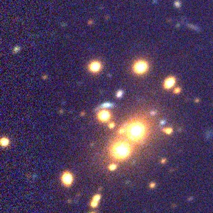
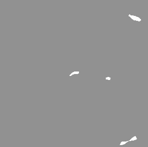
Figure 1: One of the arcs detected by More et al. (2012), in the centre, used to initialize arcfinder parameters. The arc is clearly detected and the number of false detections is very small, in comparison to all objects in the field, already at the segmentation stage, before further selection process.

3 Data set

To test our arcfinding method and possibly discover new strong lensing features, we processed stacked images belonging to the CFHTLS-Archive-Research Survey (CARS) (Erben et al., 2009), a set of three high-galactic-latitude patches covering a total of 37 $deg^{2}$ and produced with the publicly available observations obtained with the MegaPrime camera mounted an the Canada-France-Hawaii Telescope (CFHT) within the Canada-France-Hawaii-Telescope Legacy Survey. The MegaPrime is an optical camera with a mosaic of $9$ CCDs of $2048$ pixels, each sampling 0.186 arcseconds over a field of view of one square degree (see e.g. Boulade et al., 2003). All observations were obtained through the filters $u^{\star}$, $g^{\prime}$, $r^{\prime}$, $i^{\prime}$ and $z^{\prime}$. The three patches of sky covered by CARS are:

field	RA	Dec.	area ($deg^{2}$)
W1	02:18:00	−07:00:00	21
W3	14:17:54	+54:30:31	5
W4	22:13:18	+01:19:00	11

The deep co-added images were produced using the GaBoDS/THELI pipeline on a pointing/colour basis after rejecting all exposures with a problematic CFHT quality assessment (Erben et al., 2005). All details about CARS can be found in Erben et al. (2009).

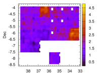
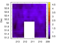
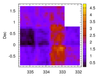
Figure 2: Maps representing the number density per $arcmin^{2}$ of all objects identified by the arcfinder before applying geometrical and colour selection criteria, which will be applied in subsequent steps to identify the arc candidates. Since the more stringent constraints are not yet applied, these maps are dominated by spurious detections, thus showing their distribution in the survey. The fluctuations in number density are expected because of the intrinsic inhomogeneous distribution of the sources and the large inhomogeneities of the image depth across the survey. We cope with this by measuring the noise locally. The three CARS fields, W1, W3 and W4, are shown.

The depth of images (AB magnitude), defined as the $5\sigma$ detection limit in a $2^{\prime\prime}$ radius aperture, is typically 25.24, 25.30, 24.36, 24.68 and 23.20 for the $u^{\star}$, $g^{\prime}$, $r^{\prime}$, $i^{\prime}$, and $z^{\prime}$ bands, respectively. The measured seeing for all co-added images is well below 1.0 arcsecond in all bands, except for the W1p3p3 $u^{\star}$-band image, having a seeing of 1.1 arcseconds, which therefore was ignored in this work. The seeing quality is crucial to detect arcs because of their very small width. A large seeing would strongly affect their signal-to-noise ratio and reduce the $L/W$ ratio, which being their most distinctive signature would make the detection significantly more difficult.

In addition to the publicly available data, we use the $g^{\prime}$ and $r^{\prime}$ bands to produce a weighted co-addition for each field to obtain a higher signal-to-noise ratio image, over which we run the arcfinder segmentation, as will be discussed later. In the co-addition, we ignored the $u^{\star}$ and $z^{\prime}$ bands because of their smaller intrinsic depth, and the $i^{\prime}$ band because of large elliptical galaxies being too prominent. Arcs tend to be close to such objects and would likely blend with them, strongly affecting their segmentation.

4 Image segmentation

As a first step of searching for gravitational arcs, we adopted the arcfinder described in Seidel & Bartelmann (2007) to produce the image segmentation necessary to detect elongated objects, and obtain important geometrical information, such as their length, $L$, and length-to-width ratio, $L/W$. Both are fundamental quantities for a subsequent object selection. In this work we briefly summarize the arcfinder algorithm in Appendix (A).

We calibrated the arcfinder parameters on an empirical basis by selecting cut-outs centred on arcs previously discovered in the CARS data, and by adjusting parameters so that arcs are recognised as such. At the same time, we controlled and evaluated the number of spurious detections to minimize their presence. At this stage, we set the final segmentation parameters but defined only very relaxed geometrical constraints, i.e. length and length-to-width ratio, for the very first selection of suitable sources. This is to obtain a wide overview of statistics of their geometrical properties to gain the necessary information for the actual calibration of the arcfinder as discussed in the next paragraphs. As an additional rejection criterion we removed circular areas surrounding bright stars, which might create false detections because of their halos and diffraction spikes. The radius in pixels, $r=420\,f^{1/3}$, of these areas is related to the stellar flux, $f$, as derived from the UCAC3 catalogue (Zacharias et al., 2010). The same catalogue is also used to define their locations in the field of view. Moreover, we set an upper limit in the surface brightness of candidates, because arcs tend to be faint. This limit is set to $0.6ADU/s$, and was empirically chosen given the surface brightnesses of the arcs used in the calibration. The most important parameters used for the segmentation are listed in Appendix (A). These parameters could be refined by iterating the process of inclusion of new arcs discovered at each step. This might be strictly necessary if none or only few known arcs are present in the field under investigation. In our case we have a sufficiently large sample for a proper and robust calibration. In fact, with a unique set of parameters, we detected arcs with very different shapes, length-to-width ratios, curvature and environment, ranging from cluster to galactic arcs.

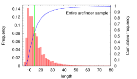
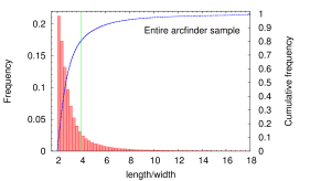
Figure 3: Probability distribution (filled bars) and cumulative function (blue line) of the length, expressed in pixels of $0.186$ arcsec in size, and the length-to-width ratio of all objects detected with the arcfinder before the application of the final geometrical and colour selection, in the left and right panels, respectively. The vertical green lines represent the respective lower limits adopted for the final candidates selection to maximize the completeness given the limits imposed by the data PSF.

In Figure (1) we present a small portion of one of the cut-outs used for the calibration together with the related segmentation produced by the arcfinder. Clearly, only very few objects appear on the right panel of the figure. Detected objects include a giant arc in the middle, one object facing edge-on, and an elongated feature resulting from blending of two objects. Blending of the lower right detection may appear excessive, given the large separation of the two objects, but we have to keep in mind that the segmentation is not based on a brightness cut-off criterion as in the case of many other algorithms. In ours, the segmentation algorithm measures coherent patterns in local second brightness moments which, for these two objects, is aligned along a common direction resulting in their merging as a single detection. We use an aggressive parameter for blending to avoid splitting of arcs with strong luminosity variations along their major axis.

With the discussed segmentation and very loose filtering applied so far to the CARS data, with very relaxed geometrical constraints used to acquire a wide statistical understanding of the data (the final selection still has to come), we obtained an initial sample of $201\,699$ sources, the number density of which across the survey is shown in Figure (2). The clear fluctuations in number density follow the intrinsic variations of the object distribution and, more importantly, depend on the large variations of the image depth across the survey field. We account for these variations during the arcfinding process, where we perform a local estimate of the noise level to retrieve a sample with uniform signal-to-noise ratio properties. Note that this initial catalogue is largely dominated by spurious objects, since the most stringent constraints are not yet applied. In Figure (3) we plot the probability distribution and cumulative function of the main geometrical properties, i.e. length and length-to-width ratio, of the entire sample of sources obtained with the arcfinder.

In this step, we aim at completeness by setting only weak constraints on the detection shapes we expect from strong lensing in combination with the PSF convolution, hence we choose a minimal length-to-width ratio of $L/W>4$ instead of bolder values, e.g. $7$ or $10$, typical for well resolved strong lensing features. Lower values cannot be adopted, as they are typical for most of the sources in the field (e.g. galaxies, amongst others). The lack of an additional length constraint would allow for objects smaller than the image PSF. Because of this reason, we set a minimum length of $L>15$ pixels (2.9 arcsec). These constraints are shown as green vertical lines in Figure (3). With these selection parameters we reduced the sample size to $36\,026$ objects, i.e. an average of about $970$ detections per square degree. This is the final sample as provided by the arcfinder when applied onto a single band. Even if the number of candidates seems large (and in fact it still contains a large number of false detections), we have to keep in mind that we started with $7\>10^{6}$ objects detected with SExtractor within the survey (Bertin & Arnouts, 1996) and that we search for objects down to the noise limit. This shows how, with the arc segmentation alone, we already have an efficient and powerful filter, even if not sufficient to obtain a reliable automatic procedure. In the next section we show how expanding the method onto three bands improves the situation.

5 Colour properties of the sample

Once we obtain the source segmentation, curvature, length and $L/W$ ratio, we get a sample of objects with the right geometrical properties, i.e. faint, thin and elongated sources. This is however still not enough for a clear distinction between gravitational arcs and other astrophysical sources or noise fluctuations. In this work we address this issue with photometry, in particular of colours. We show, in fact, that the population of sources with the largest probability to experience strong lensing (thus resulting in gravitational arcs) is dominated by a fairly uniform population of galaxies at redshift $z\approx 1$. These objects are mainly small galaxies with large star forming regions and therefore specific colour properties (Willmer et al., 2006).

5.1 Theoretical motivation

The probability of observing sources with strong lensing features is given by their number-density distribution dependent on redshift,

$$n(z)=\frac{z^{a}}{z^{b}+c\,z^{2}+d}\;,$$ (5)

where $a=1.79$, $b=0.17$, $c=8.62$, $d=0.03$, which is the redshift distribution proposed by Benjamin et al. (2007) with an additional term in the denominator, and the lensing cross section of an intervening lens,

$$\sigma_{\rm d}(z_{s})=\eta^{2}\int_{B_{\rm l}}\frac{\mathrm{d}^{2}x}{|\mu(x)|}\;,$$ (6)

defined as the area on the source plane, where sources are imaged as arcs with $L/W$ ratio larger than a given minimum, $d$. Here $\mu$ is the lensing magnification as introduced in Equation (4), $B_{\rm l}$ represents the area in the lens plane for which the condition $L/W>d$ is met, $x=\theta/\theta_{0}$ are dimensionless coordinates scaled by $\theta_{0}$ and $\eta_{0}=(D_{\rm s}/D_{\rm l})\theta_{0}$ in the lens and source plane, respectively. For simplicity we assume point sources and spherically symmetric lenses modelled as NFW halos (Navarro et al., 1997) with scale radii $r_{\rm s}$. The redshift distribution of the number density of expected arcs, $\Gamma_{\rm d}(z_{\rm s})=n(z_{\rm s})\;\tau(z_{\rm s})$, is obtained by multiplying the sources number density, $n(z)$, with the sum of the cross section of all lenses between the observer and the sources divided by the area of the source plane, i.e. the lensing optical depth,

$$\tau_{\rm d}(z_{s})=\frac{1}{4\pi D_{s}^{2}}\int^{z_{\rm s}}_{0}\int^{\infty}_{0}N(m,z)\,\sigma_{\rm d}(m,z,z_{s})\,\mathrm{d}z\mathrm{d}m\;.$$ (7)

Here, $N(m,z)\mathrm{d}z$ is the total number of haloes with mass $m$ enclosed in the cosmic volume within redshifts $z$ and $z+dz$ as defined by the Sheth & Tormen (2002) differential mass function. In the left and right panels of Figure (4) we show the sources distribution of the CARS galaxy sample together with the lensing optical depth, $\tau_{\rm d}$, and the resulting distribution of the arcs, $\Gamma_{\rm d}$, respectively. Here, we can safely use the redshift distribution of all sources in the survey, which is dominated by weakly lensed sources, and fully ignore their flux enhancement, which would be caused by a strong lens. This is because while lensing does increase the total flux of a source, it does not affect its surface brightness, which is what the initial arcfinder detection is more sensitive to. The peak of the number of strongly lensed sources at $z\approx 1$, is caused by the steep rise of the optical depth and the drop of the source number density with increasing redshift. The high redshift tail of our model overestimates the actual number of expected arcs because the best fit of the sources overestimates the actual data, which drop for $z>1.3$ to become zero for $z>2$. For this reason, we can assume that the largest number of strongly lensed sources in our data are confined to a relatively narrow redshift interval around $z\approx 1$.

Many different works based on numerical N-body simulations and halo-models have been devoted to the evaluation of the lensing optical depth with extended sources, the lens intrinsic ellipticity and the presence of substructures within large haloes (see e.g. Meneghetti et al., 2003; Li et al., 2005; Fedeli et al., 2006). These additional details mostly increase the efficiency of lenses to produce arcs and only marginally affect its redshift dependence, which we are interested in. With our simple model we just focus the attention on the sources rather than on the lenses, in contrast to most of these studies. It is neither meant to produce a detailed prediction of the number of observable arcs nor to define the actual parameters used to perform the object identification. Here, we highlight the priciples which motivate our selection criteria aiming at the objects with the highest probability to be strongly lensed, i.e. those at $z\approx 1$. The actual selection will be performed by calibrating the method on the colours of known arcs as it will be detailed in the following section.

Figure 4: Left panel: Lensing optical depth, $\tau_{\rm d}$, based on NFW haloes following the Sheth & Tormen (2002) differential mass function, together with the actual data and best fit of the CARS source redshift distribution, $n(z_{\rm s})$. Right panel: redshift distribution of the expected number density of arcs, $\Gamma_{\rm d}$, based on the best fit of the sources’ redshift distribution. Note that the best fit of the source distribution used in this model overestimates the actual counts which drop for $z>1.3$ and vanish at $z\approx 2$, thus suppressing the high redshift tail of $\Gamma_{\rm d}$. The vertical line marks the redshift limit of the observable sources.

5.2 Observational evidence

To substantiate our line of argument, we measured photometric properties of the entire sample for all available bands. Magnitudes were measured via aperture photometry

$$m=ZP-2.5\;\log_{10}(I-S\,A)\;,$$ (8)

where $ZP$ is the zero-point magnitude (as given in the CARS fits headers), $I$ is the total flux in the aperture given in ADUs, $A$ is the number of pixels within the aperture, and $S=2.5\;median-1.5\;mean$ is the background mode (Bertin & Arnouts, 1996) evaluated on the area enclosed within $4.5$ arcsec from the outer edge of the aperture. The so-defined background correction accounts for a possible flux contribution of the lens candidate, which should be close to the arc it produces. This implicitly assumes that the lens light profile decreases linearly in the immediate vicinity of the arc, as justified by its small width. We remind the reader that the aperture of each individual object is defined by the segmentation produced with the arcfinder from the weighted stack of the $g^{\prime}$ and $r^{\prime}$ images (see Section 3), and is kept fixed for all bands.

In the left panel of Figure (5) we plotted a colour-colour diagram ($g-r$,$r-i$) showing, as red circles, the most evident arcs already known in the literature (More et al., 2012) for which we could derive photometry based on the arcfinder segmentation. The other points refer to a sub-sample of galaxies, grouped in redshift bins, observed with the SUBARU telescope in the COSMOS field (Ilbert et al., 2009). The colour redshift dependence of the galaxies is clear, and shows how lensed sources are indeed associated to galaxies at redshift $z\approx 1$, as expected. The black arrow represents colours of a Scd galaxy, with large spiral arms dominated by a population of young stars for redshifts ranging from $z=0.7$ (start of line) to $z=1.3$ (arrowhead), as derived from a synthetic spectral energy distribution (SED) produced by Coleman et al. (1980). This is not used to define the colour cuts but to show the region where we expect to find galaxies with bright star-forming regions and therefore well defined colour properties. In the right panel of Figure (5) we repeated the same exercise, but with all sources detected by the arcfinder. It is visible how the covered by the arcs excludes a very large fraction of sources (number density is shown in the background), helping to drastically reduce sample contamination. With these arguments, supported by our theoretical model and data alike, we now have a robust basis to help us in distinguishing arcs from other astrophysical sources. We favour this simple colour based method in contrast to a full photometric redshift estimate, because the redshift catalogues available in the literature are not well tailored for the task. This is because usually adopted segmentation and de-blending are likely to merge arcs with relatively bright galaxies to which they are associated, resulting in misleading and largely incomplete results. The colour selection is sufficient to constrain the redshift range which has to be investigated.

We can now proceed to define colour selection, where for convenience we use the flux related quantity

$$f_{x}=A^{-1}\,10^{\,0.4\,(K-m_{x})}\;,$$ (9)

to express the difference in flux over area for neighbouring bands in the fashion of usual colour-colour plots, instead of the typical definition based on magnitudes. Here, $m_{x}$ is the object magnitude in $x$-band, where $x$ stands for $x=[u^{\star},g^{\prime},r^{\prime},i^{\prime},z^{\prime}]$, and $K=26.42$ is the magnitude average of all sources in the $r^{\prime}$-band resulting in a multiplicative factor introduced for convenience.

In this “colour-colour” space, based on Equation (9), the arcs previously known in the survey, and plotted in Figures (5) and (6) as red circles, appear nicely aligned along a relatively narrow region in colour-colour space. These objects were used to define the region, marked with red lines in Figure (6), that we used to select other arc candidates. In the same figure we also plot the objects we identified in the survey as arcs, where details will be given in Section (6). For the moment, it shall suffice to say that all objects marked in these plots were not selected according to their colour properties, making them an independent check sample. These detections as well predominantly populate the same colour-colour space we used to define the colour selection, lending further support to the validity of our approach.

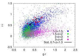
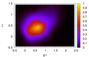
Figure 5: Left panel shows a colour-colour diagram for previously known arcs, in red, and a sub-sample of galaxies observed in the COSMOS field subdivided in redshift bins. The red points denote the arcs previously known in the survey and which are used to calibrate the colour selection. The small colour region where arcs are present shows how the lensed sources lie at redshift $z\approx 1$ (as predicted by our optical depth model) and have well defined colour properties (as shown by the black arrow referring to a Scd galaxy, for which we derived the photometry out of a synthetic SED, here the arrowhead points in the direction of increasing redshifts). The right panel shows the same colour-colour diagram, but for all objects detected by the arcfinder.

It is difficult to extract detailed statistics from the small sample of known arcs, hence we decided not to use a more sophisticated colour selection criterion. The sample of detections after the colour selection reduces to $5\,597$ candidates, i.e. approximately 150 per square degree, versus 970 per square degree in the catalogue obtained with the single-band arcfinder, with comparatively less contamination. This colour selection clearly restricts the detection of arcs to a certain type of lensed sources. Nevertheless, we do not consider this as a limitation, because (1) we expect the population of lensed sources selected in this way to be the most numerous, ensuring that only a small fraction of arcs is lost, as will be shown later in the text, (2) sources and lenses are completely uncorrelated, because of their large relative separation, avoiding any bias which may be due to physical correlations, and (3) gravitational lensing is a completely achromatic phenomenon independent of the colour of the sources. The giant arcs count, used to infer cosmological information, depends on this colour selection, but this can be easily accounted for just by applying the same colour selection to the expected number density of background sources, which is a trivial task.

6 Visual validation and catalogue

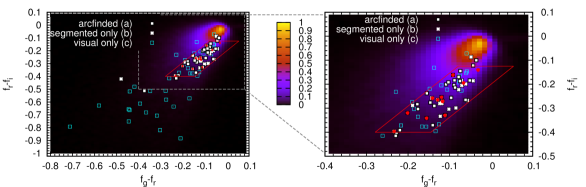
Figure 6: Flux related “colour-colour” space for all arcfinder detections (background intensity), the previously known arcs present in the field for which we derived their photometry (red points), and the region, within the red lines, used to select the final arcs sample. The white squares (a) are the candidates detected by the arcfinder, the white asterisks (b) are those segmented by the arcfinder but rejected by its geometrical filters and the cyan void squares (c) are those found purely by visual inspection. The latter are the most difficult sources and are scattered in a very wide area, far from most of the other sources, because of their uncertain photometry.

The candidates produced with the discussed procedure are finally verified by visually inspecting their colour composite images obtained using the $g^{\prime}$, $r^{\prime}$ and $i^{\prime}$ bands. We associated a rank to each detection based on three levels:

• 1=unlikely: arc structures which seem physically associated to an astrophysical object, or which are relatively far from a possible lens,

• 2=unclear: arc structures with a very promising shape, but still of dubious origin,

• 3=very likely: a clear curved arc structure around a possible lens causing its origin, i.e. large ellipticals or significant concentrations of galaxies.

A rank $0$ is also used to label artefacts, evident spiral galaxies, or clear noise fluctuations. This simple ranking yields stable results with respecto to different observers and even the same observer but at different times. In addition we also inspected the full survey to evaluate the completeness and purity of the sample against a full visual investigation. This very important topic will be covered in Section (7).

The final catalogue listing all arcs with rank $r\geq 2$ is shown in Tables (1, 2 and 3) with their positions, geometrical properties, photometry, redshifts and ranks. The first two tables contain the 56 detections satisfying the colour criterion, while the 34 detections in the third table, most of them found only by visual inspection, do not. The candidates detected by the arcfinder, i.e satisfying the tight geometrical constraints, are labelled with ‘a’. Only five of them do not meet the colour criterion. Three of those (arc58a, arc59a, arc60a) are located in the vicinity of very bright stars whose halos might have spoiled their photometry, and one (arc61a) belongs to a complex object of unclear nature, possibly showing multiple arcs. The objects segmented by the arcfinder but discarded by it because they do not fulfil the geometrical constraints are labelled with ‘b’ and all but three of them satisfy the colour constraints. Finally, the candidates detected via eye-ball checking the whole survey and missed entirely by the arcfinder are labelled with ‘c’. The majority of the visually identified objects fall into Table (3) of detections rejected by the colour selection because of their low surface brightness and heavy blending, which makes them generally the most difficult candidates to find. The complete sample consists of 90 objects, 73 of which are newly proposed arc candidates. Postage stamp cut-outs of their images are available online.

We obtained more candidates with respect to those proposed by More et al. (2012) and Cabanac et al. (2007) not only because of the different arcfinder adopted but also because of the different selection criteria and because they restricted their sample with respect to the arc-lens separation to $r>14$ arcsec. Note that we dropped two of their candidates, i.e. SA98 and SL2SJ021932-053135, which in our opinion are not lensing features but structures physically associated to the galaxy believed to be the lens in the first case, and a spiral arm of a nearby galaxy in the latter. The arcfinder used in this work clearly detected SA38, but this was rejected because of its high luminosity exceeding the maximum we allowed.

Table 1: Final gravitational arc candidates satisfying the colour criteria. Detections with $RANK\leq 1$, i.e. clear artefacts or features possibly related to spiral galaxies or tidal streams, are not listed. The objects labelled with ‘a’ were detected by the arcfinder Those labelled with ‘b’ were segmented by the arcfinder but rejected by our tight geometrical constraints. Those labelled with ‘c’ were detected only via eye-ball checking. The table lists: the arc identification number ‘ID’, the CARS field ‘FIELD’, the Right Ascension and Declination, ‘RA’ and ‘DEC’, the arc length ‘LEN’ in arcsec, the length-to-width ratio ‘L/W’, the curvature ‘CUR’ in $\rm arcsec^{-1}$, the area ‘A’ in $\rm arcsec^{2}$, the $u^{\star}$,$g^{\prime}$,$r^{\prime}$,$i^{\prime}$ magnitudes, the lens redshift ‘$z_{\rm lens}$’, the arc candidate redshift ‘$z_{\rm arc}$’, the detection ranking ‘RANK’, and the identification number in More et al. (2012) or Cabanac et al. (2007) if present. The arc redshift is enclosed within brackets to stress its low reliability.

ID	FIELD	RA	DEC	LEN	L/W	CUR	A	mu′	mg′	mr′	mi′	zlens	RANK	CAT
arc1a	W1m1p1	02:13:17.2	-06:25:58	2.91	4.66	0.21	2.0	$25.6^{\pm 0.6}$	$24.3^{\pm 0.2}$	$23.7^{\pm 0.5}$	$23.1^{\pm 0.2}$	$0.39_{-0.09}^{+0.09}$	2	-
arc2a	W1m1p2	02:14:08.0	-05:35:27	7.92	8.65	0.14	8.1	$23.0^{\pm 0.2}$	$22.3^{\pm 0.1}$	$21.6^{\pm 0.1}$	$21.0^{\pm 0.1}$	$0.49_{-0.21}^{+0.22}$	3	SA22
arc3a	W1m1p1	02:14:40.5	-06:31:16	4.56	5.06	0.18	4.0	$24.7^{\pm 0.3}$	$23.8^{\pm 0.1}$	$23.1^{\pm 0.2}$	$22.3^{\pm 0.1}$	$0.34_{-0.09}^{+0.09}$	2	-
arc4a	W1m1p1	02:16:00.2	-05:57:04	4.08	4.82	0.18	3.6	$25.1^{\pm 0.4}$	$24.0^{\pm 0.2}$	$23.1^{\pm 0.3}$	$22.4^{\pm 0.1}$	$0.36_{-0.09}^{+0.09}$	2	-
arc5a	W1m0p3	02:17:13.2	-04:01:13	4.28	5.92	0.73	3.5	$24.7^{\pm 0.4}$	$24.2^{\pm 0.2}$	$23.5^{\pm 0.3}$	$22.6^{\pm 0.1}$	$0.68_{-0.11}^{+0.11}$	2	-
arc6a	W1m0p2	02:18:05.0	-05:19:49	5.53	4.23	0.28	6.5	$23.2^{\pm 0.2}$	$22.8^{\pm 0.1}$	$22.4^{\pm 0.1}$	$21.5^{\pm 0.1}$	$0.77_{-0.12}^{+0.12}$	2	-
arc7a	W1m0p1	02:19:03.9	-05:51:25	4.03	5.15	0.00	3.7	$25.1^{\pm 0.6}$	$24.2^{\pm 0.2}$	$23.3^{\pm 0.2}$	$22.3^{\pm 0.1}$	$0.44_{-0.09}^{+0.09}$	2	-
arc8a	W1m0p3	02:19:09.6	-04:01:43	5.66	4.90	0.12	5.9	$24.1^{\pm 0.3}$	$23.3^{\pm 0.1}$	$22.5^{\pm 0.1}$	$21.7^{\pm 0.1}$	$0.33_{-0.09}^{+0.09}$	3	SA35
arc9a	W1m0p3	02:19:37.5	-04:16:18	3.59	4.57	0.23	3.0	$24.4^{\pm 0.3}$	$23.9^{\pm 0.1}$	$23.5^{\pm 0.3}$	$22.7^{\pm 0.1}$	$0.49_{-0.21}^{+0.22}$	2	-
arc10a	W1m0p2	02:19:56.4	-05:27:56	3.73	4.83	0.21	2.9	$23.8^{\pm 0.2}$	$23.0^{\pm 0.1}$	$22.4^{\pm 0.1}$	$21.8^{\pm 0.1}$	$0.32_{-0.09}^{+0.09}$	3	SA36
arc11a	W1p1p1	02:20:44.4	-05:37:46	4.34	4.76	0.07	4.1	$24.4^{\pm 0.3}$	$23.4^{\pm 0.1}$	$22.9^{\pm 0.2}$	$22.1^{\pm 0.1}$	$0.72_{-0.11}^{+0.11}$	2	-
arc12a	W1p1p3	02:21:34.5	-04:24:38	7.44	12.03	0.32	6.0	$23.5^{\pm 0.2}$	$22.6^{\pm 0.1}$	$22.0^{\pm 0.1}$	$21.3^{\pm 0.1}$	$0.70_{-0.11}^{+0.11}$	3	-
arc13a	W1p2p2	02:25:32.0	-04:50:59	5.49	8.20	0.37	4.4	$23.2^{\pm 0.2}$	$22.6^{\pm 0.1}$	$21.9^{\pm 0.1}$	$21.3^{\pm 0.1}$	$0.62_{-0.11}^{+0.11}$	2	SL2SJ022532-045100
arc14a	W1p3p1	02:31:06.7	-05:55:02	3.52	4.50	0.51	2.8	$25.1^{\pm 0.5}$	$24.1^{\pm 0.2}$	$23.4^{\pm 0.4}$	$22.8^{\pm 0.2}$	$0.53_{-0.10}^{+0.10}$	3	SA57
arc15a	W3m3m2	14:00:21.2	+52:15:47	7.21	10.00	0.40	6.2	$23.1^{\pm 0.2}$	$22.3^{\pm 0.1}$	$21.8^{\pm 0.1}$	$21.1^{\pm 0.1}$	$0.76_{-0.12}^{+0.12}$	2	-
arc16a	W3m3m2	14:01:44.6	+53:02:09	3.67	4.20	0.13	3.5	$24.0^{\pm 0.2}$	$23.4^{\pm 0.1}$	$22.8^{\pm 0.2}$	$22.0^{\pm 0.1}$	$0.47_{-0.10}^{+0.10}$	3	SA91
arc17a	W4m1m2	22:09:18.3	+00:50:03	3.17	4.16	0.45	2.4	$25.3^{\pm 0.5}$	$23.7^{\pm 0.2}$	$23.0^{\pm 0.3}$	$22.4^{\pm 0.1}$	$0.49_{-0.21}^{+0.22}$	2	-
arc18a	W4m0m0	22:12:22.0	+01:36:46	4.08	4.61	0.37	4.4	$24.5^{\pm 0.3}$	$23.7^{\pm 0.1}$	$23.1^{\pm 0.2}$	$22.4^{\pm 0.1}$	$0.72_{-0.11}^{+0.11}$	3	-
arc19a	W4m0m1	22:12:55.3	+00:17:07	6.37	6.34	0.24	6.7	$24.0^{\pm 0.2}$	$23.0^{\pm 0.1}$	$22.2^{\pm 0.1}$	$21.4^{\pm 0.1}$	$0.58_{-0.10}^{+0.10}$	2	-
arc20a	W4m0m2	22:13:06.9	+00:18:30	5.34	4.26	0.20	5.9	$23.8^{\pm 0.2}$	$22.9^{\pm 0.1}$	$22.3^{\pm 0.1}$	$21.7^{\pm 0.1}$	$0.49_{-0.21}^{+0.22}$	3	-
arc21a	W4m0m0	22:13:14.2	+00:50:09	7.80	6.08	0.15	8.2	$24.6^{\pm 0.3}$	$23.4^{\pm 0.1}$	$22.5^{\pm 0.1}$	$21.6^{\pm 0.1}$	$0.45_{-0.10}^{+0.10}$	2	-
arc22a	W4m0m0	22:14:18.9	+01:10:35	6.14	8.76	0.60	4.9	$24.4^{\pm 0.3}$	$23.3^{\pm 0.1}$	$22.4^{\pm 0.2}$	$21.6^{\pm 0.1}$	$0.56_{-0.10}^{+0.10}$	3	SA125
arc23a	W4p1m0	22:15:13.4	+01:02:41	6.85	6.62	0.07	7.3	$23.8^{\pm 0.3}$	$22.7^{\pm 0.1}$	$22.1^{\pm 0.1}$	$21.2^{\pm 0.1}$	$0.69_{-0.11}^{+0.11}$	2	-
arc24a	W4p1m2	22:16:58.7	+00:01:53	3.99	5.65	0.00	2.9	$24.2^{\pm 0.4}$	$23.4^{\pm 0.2}$	$22.7^{\pm 0.2}$	$22.1^{\pm 0.1}$	$0.67_{-0.11}^{+0.11}$	2	-
arc25b	W1m1p3	02:14:11.1	-04:05:03	1.68	3.24	0.33	1.2	$24.5^{\pm 0.4}$	$24.2^{\pm 0.2}$	$23.9^{\pm 0.3}$	$23.1^{\pm 0.2}$	$0.77_{-0.12}^{+0.12}$	3	SA23
arc26b	W1m1p1	02:14:26.4	-05:39:39	3.73	3.56	0.19	3.8	$24.6^{\pm 0.3}$	$23.7^{\pm 0.1}$	$22.9^{\pm 0.2}$	$22.0^{\pm 0.1}$	$0.55_{-0.10}^{+0.10}$	2	-
arc27b	W1m0p2	02:16:06.4	-04:49:35	4.19	2.53	0.52	5.7	$23.8^{\pm 0.2}$	$23.4^{\pm 0.1}$	$22.9^{\pm 0.1}$	$22.0^{\pm 0.1}$	$0.30_{-0.09}^{+0.14}$	3	-
arc28b	W1m0p2	02:17:37.4	-05:13:30	2.72	2.76	0.21	2.8	$24.8^{\pm 0.4}$	$24.1^{\pm 0.2}$	$23.7^{\pm 0.4}$	$22.8^{\pm 0.2}$	$0.82_{-0.12}^{+0.12}$	3	SL2SJ021737-051329
arc29b	W1m0p2	02:18:07.4	-05:15:36	2.72	3.61	0.07	2.1	$25.5^{\pm 0.7}$	$24.0^{\pm 0.1}$	$23.4^{\pm 0.2}$	$22.6^{\pm 0.1}$	$0.60_{-0.10}^{+0.11}$	3	SA33
arc30b	W1m0p1	02:19:28.3	-05:44:59	2.00	2.33	0.45	1.7	$25.2^{\pm 0.6}$	$24.3^{\pm 0.3}$	$23.9^{\pm 0.4}$	$23.2^{\pm 0.2}$	$0.26_{-0.08}^{+0.08}$	3	-

Table 2: Continued from Table (1).

ID	FIELD	RA	DEC	LEN	L/W	CUR	A	mu′	mg′	mr′	mi′	zlens	RANK	CAT
arc31b	W1p1p1	02:21:14.9	-05:42:42	1.92	2.05	0.27	2.1	$24.7^{\pm 0.4}$	$23.6^{\pm 0.1}$	$22.9^{\pm 0.3}$	$22.3^{\pm 0.1}$	$0.28_{-0.08}^{+0.09}$	2	-
arc32b	W1p1p1	02:23:15.3	-06:29:03	2.33	3.39	0.26	2.0	$24.9^{\pm 0.4}$	$23.6^{\pm 0.1}$	$22.9^{\pm 0.1}$	$22.2^{\pm 0.1}$	$0.57_{-0.10}^{+0.10}$	3	SA40
arc33b	W1p2p2	02:24:27.3	-04:55:43	1.34	2.01	0.21	1.0	$25.2^{\pm 0.6}$	$24.4^{\pm 0.2}$	$23.9^{\pm 0.5}$	$23.3^{\pm 0.2}$	$0.56_{-0.10}^{+0.10}$	3	-
arc34b	W1p4p3	02:33:07.2	-04:38:38	2.23	3.98	0.11	1.5	$25.5^{\pm 0.7}$	$24.1^{\pm 0.2}$	$23.6^{\pm 0.3}$	$22.9^{\pm 0.2}$	$0.66_{-0.11}^{+0.11}$	3	SA59
arc35b	W3m3m2	13:57:02.4	+52:30:39	2.43	4.71	0.17	1.6	$25.7^{\pm 0.8}$	$24.7^{\pm 0.4}$	$23.8^{\pm 0.6}$	$23.0^{\pm 0.3}$	$0.38_{-0.09}^{+0.09}$	3	-
arc36b	W3m3m2	13:58:22.4	+52:43:19	2.56	2.93	0.31	2.3	$23.9^{\pm 0.2}$	$23.5^{\pm 0.1}$	$23.2^{\pm 0.3}$	$22.5^{\pm 0.2}$	$0.55_{-0.10}^{+0.10}$	3	-
arc37b	W3m3m2	13:58:46.6	+52:21:00	1.58	2.25	0.00	1.1	$26.2^{\pm 1.3}$	$24.9^{\pm 0.4}$	$24.2^{\pm 0.8}$	$23.4^{\pm 0.3}$	$0.35_{-0.09}^{+0.09}$	2	-
arc38b	W4m0m1	22:12:29.9	+00:17:25	2.47	2.80	0.00	2.4	$24.6^{\pm 0.5}$	$23.5^{\pm 0.1}$	$23.1^{\pm 0.3}$	$22.3^{\pm 0.1}$	$0.58_{-0.10}^{+0.10}$	3	-
arc39b	W4m0m2	22:13:07.1	+00:30:37	3.06	3.75	0.32	2.5	$24.9^{\pm 0.4}$	$24.1^{\pm 0.1}$	$23.3^{\pm 0.3}$	$22.4^{\pm 0.1}$	$0.58_{-0.10}^{+0.10}$	3	SA122
arc40b	W4p2m2	22:20:18.6	+00:24:28	2.56	2.80	1.01	2.1	$25.2^{\pm 0.6}$	$24.4^{\pm 0.3}$	$23.9^{\pm 0.6}$	$23.0^{\pm 0.1}$	$0.52_{-0.10}^{+0.10}$	2	-
arc41b	W4p2m1	22:21:41.8	+00:19:09	2.15	2.65	0.56	1.8	$24.6^{\pm 0.3}$	$23.4^{\pm 0.1}$	$23.1^{\pm 0.2}$	$22.7^{\pm 0.1}$	$0.64_{-0.11}^{+0.11}$	2	-
arc42c	W1m1p1	02:12:31.6	-06:11:54	7.56	7.33	0.18	8.5	$25.4^{\pm 0.5}$	$23.9^{\pm 0.1}$	$22.8^{\pm 0.2}$	$21.8^{\pm 0.1}$	$0.36_{-0.09}^{+0.09}$	3	-
arc43c	W1m1p3	02:15:13.5	-03:53:44	3.17	3.52	0.11	3.0	$24.8^{\pm 0.5}$	$24.1^{\pm 0.2}$	$23.0^{\pm 0.2}$	$22.1^{\pm 0.1}$	$0.51_{-0.11}^{+0.10}$	2	-
arc44c	W1m1p3	02:15:57.1	-04:10:27	2.19	2.20	1.10	1.9	$24.7^{\pm 0.5}$	$24.1^{\pm 0.2}$	$23.1^{\pm 0.2}$	$22.4^{\pm 0.1}$	$0.82_{-0.12}^{+0.12}$	3	-
arc45c	W1m0p1	02:19:32.7	-06:28:44	3.71	3.54	0.32	4.5	$25.2^{\pm 0.5}$	$24.5^{\pm 0.3}$	$23.4^{\pm 0.2}$	$22.4^{\pm 0.2}$	$0.65_{-0.11}^{+0.11}$	2	-
arc46c	W1p3p1	02:29:32.1	-06:15:32	2.22	2.02	0.00	2.4	$24.9^{\pm 0.4}$	$24.2^{\pm 0.2}$	$23.7^{\pm 0.3}$	$22.8^{\pm 0.1}$	$0.58_{-0.10}^{+0.10}$	2	-
arc47c	W3m3m3	13:57:23.9	+51:21:30	2.70	3.04	0.61	2.6	$25.6^{\pm 0.7}$	$24.3^{\pm 0.2}$	$23.4^{\pm 0.3}$	$22.3^{\pm 0.1}$	$0.60_{-0.10}^{+0.11}$	2	-
arc48c	W3m3m3	14:00:09.5	+52:06:24	4.97	5.67	0.67	7.3	$24.4^{\pm 0.3}$	$23.2^{\pm 0.1}$	$22.4^{\pm 0.1}$	$21.5^{\pm 0.1}$	$0.54_{-0.10}^{+0.10}$	2	-
arc49c	W3m3m2	14:00:28.6	+52:55:26	2.16	2.51	0.47	1.9	$25.3^{\pm 0.6}$	$24.3^{\pm 0.2}$	$23.3^{\pm 0.3}$	$22.6^{\pm 0.1}$	$0.53_{-0.12}^{+0.10}$	2	-
arc50c	W3m3m2	14:01:02.7	+52:37:23	8.06	7.55	0.30	11.0	$24.8^{\pm 0.4}$	$23.3^{\pm 0.1}$	$22.5^{\pm 0.2}$	$21.6^{\pm 0.1}$	$0.50_{-0.11}^{+0.10}$	3	-
arc51c	W3m1m3	14:12:35.8	+51:33:24	4.61	3.94	0.87	5.9	$23.9^{\pm 0.3}$	$22.8^{\pm 0.1}$	$22.0^{\pm 0.1}$	$21.2^{\pm 0.1}$	$0.74_{-0.11}^{+0.11}$	3	-
arc52c	W4m1m2	22:07:53.1	+00:39:38	6.08	4.29	0.20	8.5	$23.3^{\pm 0.2}$	$22.6^{\pm 0.1}$	$22.1^{\pm 0.1}$	$21.4^{\pm 0.1}$	$0.48_{-0.10}^{+0.10}$	2	-
arc53c	W4m1m1	22:10:33.1	+00:23:51	1.80	1.99	0.92	2.3	$25.6^{\pm 0.7}$	$24.4^{\pm 0.2}$	$23.4^{\pm 0.5}$	$22.4^{\pm 0.2}$	$0.58_{-0.10}^{+0.10}$	2	-
arc54c	W4p2m0	22:20:51.5	+00:58:14	2.49	2.07	0.30	3.3	$24.0^{\pm 0.2}$	$23.3^{\pm 0.1}$	$23.0^{\pm 0.2}$	$22.5^{\pm 0.1}$	$0.41_{-0.09}^{+0.09}$	2	-
arc55c	W4p2m2	22:21:58.5	+00:59:02	2.50	2.57	0.33	2.9	$25.4^{\pm 0.7}$	$24.2^{\pm 0.2}$	$23.5^{\pm 0.7}$	$22.8^{\pm 0.1}$	$0.33_{-0.09}^{+0.09}$	2	-
arc56c	W4p2m0	22:22:23.0	+01:16:05	4.46	4.25	0.40	4.7	$24.5^{\pm 0.6}$	$23.1^{\pm 0.2}$	$22.5^{\pm 0.3}$	$21.9^{\pm 0.1}$	$0.53_{-0.10}^{+0.10}$	2	-

Table 3: Same as Table (1) and (2) but referring to all detections not satisfying the colour criteria. This sample is mostly composed by candidates purely identified by visual inspection.

ID	FIELD	RA	DEC	LEN	L/W	CUR	A	mu′	mg′	mr′	mi′	zlens	RANK	CAT
arc57a	W1m1p2	02:14:16.6	-05:03:15	4.27	4.43	0.23	4.6	$23.5^{\pm 0.2}$	$22.8^{\pm 0.1}$	$21.7^{\pm 0.1}$	$21.0^{\pm 0.1}$	$0.37_{-0.09}^{+0.09}$	3	SL2SJ021416-050315
arc58a	W1p1p1	02:22:33.6	-06:06:24	3.33	5.41	0.00	2.3	$24.6^{\pm 0.4}$	$23.5^{\pm 0.1}$	$22.7^{\pm 0.2}$	$22.0^{\pm 0.1}$	$0.45_{-0.11}^{+0.10}$	2	-
arc59a	W1p2p3	02:24:01.0	-03:46:27	4.90	7.20	0.24	6.3	$24.6^{\pm 0.5}$	$23.5^{\pm 0.2}$	$23.1^{\pm 0.3}$	$22.4^{\pm 0.3}$	$0.81_{-0.12}^{+0.12}$	3	SA42
arc60a	W1p2p2	02:25:34.1	-05:02:10	4.88	5.16	0.30	4.7	$24.5^{\pm 0.4}$	$23.9^{\pm 0.2}$	$23.4^{\pm 0.4}$	$22.6^{\pm 0.1}$	$0.67_{-0.11}^{+0.11}$	3	-
arc61a	W3m3m3	13:59:53.7	+51:39:53	4.67	13.80	0.46	2.3	$24.5^{\pm 0.3}$	$23.4^{\pm 0.1}$	$22.7^{\pm 0.2}$	$22.0^{\pm 0.1}$	$0.53_{-0.10}^{+0.10}$	2	-
arc62b	W1p2p3	02:23:45.6	-04:24:03	2.19	2.49	0.33	2.2	$24.6^{\pm 0.3}$	$23.1^{\pm 0.1}$	$22.1^{\pm 0.1}$	$21.7^{\pm 0.1}$	$0.37_{-0.09}^{+0.09}$	2	SL2SJ022345-042402
arc63b	W1p3p2	02:28:34.3	-05:09:48	1.50	2.66	0.01	1.0	$26.2^{\pm 1.0}$	$25.4^{\pm 0.5}$	$24.9^{\pm 1.0}$	$24.4^{\pm 0.8}$	$0.57_{-0.10}^{+0.10}$	2	-
arc64b	W1p3p1	02:30:11.6	-05:50:21	3.29	3.16	0.05	3.8	$23.7^{\pm 1.7}$	$22.6^{\pm 0.2}$	$0.0^{\pm 0.1}$	$20.7^{\pm 0.1}$	$0.49_{-0.21}^{+0.22}$	3	SL2SJ023011-055023
arc65c	W1m1p1	02:12:33.8	-06:12:10	1.32	1.48	0.06	1.2	$25.5^{\pm 0.5}$	$24.1^{\pm 0.1}$	$23.0^{\pm 0.2}$	$22.3^{\pm 0.1}$	$0.31_{-0.09}^{+0.11}$	2	-
arc66c	W1m1p1	02:13:08.7	-05:37:26	3.21	3.01	0.17	3.5	$24.3^{\pm 0.2}$	$22.7^{\pm 0.1}$	$21.6^{\pm 0.1}$	$21.0^{\pm 0.1}$	$0.29_{-0.08}^{+0.08}$	2	-
arc67c	W1m1p2	02:13:28.4	-05:11:45	2.88	2.46	0.08	4.4	$24.2^{\pm 0.3}$	$23.1^{\pm 0.1}$	$21.8^{\pm 0.1}$	$21.0^{\pm 0.1}$	$0.49_{-0.10}^{+0.10}$	2	-
arc68c	W1m1p2	02:15:29.4	-04:40:54	2.36	3.25	0.18	1.8	$25.6^{\pm 1.1}$	$24.2^{\pm 0.2}$	$22.9^{\pm 0.2}$	$22.1^{\pm 0.1}$	$0.31_{-0.09}^{+0.09}$	3	-
arc69c	W1m1p1	02:15:34.8	-05:45:15	2.07	2.78	0.13	1.8	$25.7^{\pm 0.8}$	$23.9^{\pm 0.2}$	$22.6^{\pm 0.2}$	$22.0^{\pm 0.1}$	$0.31_{-0.09}^{+0.09}$	2	-
arc70c	W1m0p3	02:19:09.1	-04:02:14	7.98	4.80	0.46	11.1	$23.6^{\pm 0.2}$	$22.5^{\pm 0.1}$	$21.5^{\pm 0.1}$	$20.8^{\pm 0.1}$	$0.49_{-0.10}^{+0.10}$	3	-
arc71c	W1p1p1	02:19:56.5	-06:02:02	5.20	2.31	0.06	12.5	$23.5^{\pm 0.2}$	$22.5^{\pm 0.1}$	$21.6^{\pm 0.1}$	$20.5^{\pm 0.1}$	$0.42_{-0.09}^{+0.09}$	2	-
arc72c	W1p1m1	02:20:56.4	-07:43:10	3.55	2.79	0.32	6.1	$22.6^{\pm 0.2}$	$22.1^{\pm 0.1}$	$0.0^{\pm 0.0}$	$20.8^{\pm 0.1}$	$0.56_{-0.24}^{+0.23}$	3	-
arc73c	W1p1p1	02:21:00.3	-06:06:12	2.89	1.96	0.18	4.2	$24.2^{\pm 0.4}$	$22.3^{\pm 0.1}$	$21.1^{\pm 0.1}$	$20.5^{\pm 0.1}$	$0.26_{-0.08}^{+0.10}$	2	-
arc74c	W1p2p3	02:25:36.7	-04:15:17	1.88	2.20	0.56	1.5	$25.1^{\pm 0.4}$	$24.1^{\pm 0.2}$	$23.1^{\pm 0.1}$	$22.1^{\pm 0.1}$	$0.56_{-0.10}^{+0.10}$	2	-
arc75c	W1p2p2	02:25:38.0	-05:14:49	3.02	2.16	0.05	4.8	$24.0^{\pm 0.2}$	$22.7^{\pm 0.1}$	$21.6^{\pm 0.1}$	$21.0^{\pm 0.1}$	$0.42_{-0.10}^{+0.09}$	2	-
arc76c	W1p3p2	02:29:08.8	-05:19:54	2.99	3.76	0.12	2.6	$24.9^{\pm 0.5}$	$23.8^{\pm 0.2}$	$23.1^{\pm 0.2}$	$22.4^{\pm 0.1}$	$0.37_{-0.09}^{+0.09}$	2	-
arc77c	W1p4m0	02:32:54.3	-06:39:16	2.38	3.08	0.50	1.8	$24.8^{\pm 0.4}$	$24.2^{\pm 0.2}$	$23.8^{\pm 0.5}$	$23.5^{\pm 0.4}$	$0.60_{-0.10}^{+0.11}$	2	-
arc78c	W1p4m0	02:33:30.1	-06:51:42	6.16	6.05	0.06	7.6	$23.0^{\pm 0.2}$	$22.4^{\pm 0.1}$	$21.5^{\pm 0.1}$	$20.5^{\pm 0.1}$	$0.65_{-0.11}^{+0.11}$	1	-
arc79c	W3m3m3	13:57:39.1	+51:48:46	4.21	4.22	0.40	5.6	$24.9^{\pm 0.4}$	$23.6^{\pm 0.1}$	$22.4^{\pm 0.2}$	$21.1^{\pm 0.1}$	$0.38_{-0.09}^{+0.09}$	3	-
arc80c	W3m3m2	13:58:19.8	+52:52:53	2.73	2.37	0.08	3.1	$25.0^{\pm 0.5}$	$23.3^{\pm 0.1}$	$22.0^{\pm 0.1}$	$21.2^{\pm 0.1}$	$0.35_{-0.09}^{+0.09}$	2	-
arc81c	W3m3m2	14:02:06.4	+52:57:07	2.05	3.90	0.41	1.0	$27.4^{\pm 3.6}$	$24.9^{\pm 0.3}$	$23.7^{\pm 0.4}$	$22.5^{\pm 0.1}$	$0.51_{-0.10}^{+0.10}$	2	-
arc82c	W3m1m3	14:12:07.1	+51:29:43	3.19	3.34	0.33	3.9	$25.3^{\pm 0.7}$	$23.6^{\pm 0.1}$	$22.5^{\pm 0.1}$	$21.1^{\pm 0.1}$	$0.30_{-0.09}^{+0.13}$	2	-
arc83c	W4m1m1	22:08:51.3	+00:46:22	1.83	2.61	0.50	1.4	$24.9^{\pm 0.4}$	$23.9^{\pm 0.1}$	$22.8^{\pm 0.2}$	$22.0^{\pm 0.1}$	$0.49_{-0.21}^{+0.22}$	2	-
arc84c	W4m1m2	22:09:35.5	+00:31:26	9.09	6.08	0.16	13.0	$24.0^{\pm 0.2}$	$22.2^{\pm 0.1}$	$21.4^{\pm 0.1}$	$21.0^{\pm 0.1}$	$0.32_{-0.09}^{+0.09}$	2	-
arc85c	W4m0m1	22:12:35.5	+00:43:11	3.75	2.92	0.77	4.7	$23.9^{\pm 0.2}$	$22.9^{\pm 0.1}$	$22.0^{\pm 0.1}$	$21.6^{\pm 0.1}$	$0.29_{-0.08}^{+0.11}$	2	-
arc86c	W4m0m2	22:13:28.9	+00:44:53	5.99	8.24	0.42	4.8	$24.7^{\pm 0.3}$	$23.4^{\pm 0.1}$	$22.1^{\pm 0.1}$	$21.1^{\pm 0.1}$	$0.38_{-0.09}^{+0.09}$	3	-
arc87c	W4m0m1	22:15:02.6	+00:49:50	3.74	3.69	0.53	3.8	$25.0^{\pm 0.4}$	$23.7^{\pm 0.1}$	$22.3^{\pm 0.1}$	$21.4^{\pm 0.1}$	$0.51_{-0.10}^{+0.10}$	3	-
arc88c	W4p1m1	22:18:21.1	+00:01:53	2.00	1.60	0.58	2.8	$23.9^{\pm 0.2}$	$23.1^{\pm 0.1}$	$22.4^{\pm 0.1}$	$21.7^{\pm 0.1}$	$0.50_{-0.10}^{+0.10}$	3	-
arc89c	W4p2m2	22:19:00.9	+00:54:56	2.58	2.24	0.19	2.7	$24.9^{\pm 0.8}$	$22.5^{\pm 0.2}$	$21.3^{\pm 0.3}$	$20.4^{\pm 0.1}$	$0.46_{-0.10}^{+0.10}$	2	-
arc90c	W4p2m1	22:22:17.6	+00:12:02	2.19	2.57	0.45	2.1	$24.9^{\pm 0.4}$	$23.5^{\pm 0.1}$	$22.5^{\pm 0.1}$	$21.7^{\pm 0.1}$	$0.51_{-0.10}^{+0.10}$	3	-

Table 4: Completeness of the final arc candidates sample listed in Tables (1, 2 and 3), comparing the results obtained before and after the colour selection. Columns refer to the objects detected by the arcfinder (arcf., labelled with ‘a’), those segmented but not recognized as arcs by the arcfinder (arcf. seg., labelled with ‘b’), those identified with the visual inspection only (visual only, labelled with ‘c’ in the sample catalogue) and the complete sample (all). This demonstrates how the colour selection looses only 17% of the single-band arcfinder sample (first column). The loss is greater when the visual detections are included, 48%, since many of those have poor photometry, being blended, faint or fragmented (last column).

	arcf. (a)	arcf. seg. (b)	visual only (c)	all
before col. sel.	29	20	41	90
after col. sel.	24	17	15	56
completeness	83%	85%	36%	62%

7 Completeness and purity of the colour-selected sample

We now evaluate the completeness and contamination of the sample, discussed in Section (6) for these three candidate subsamples:

1. 29 objects, among 36 026 detected by the arcfinder

2. 20 objects, among 165 673 segmented but discarded by the arcfinder’s morphological filter,

3. 41 objects identified only with the visual inspection,

and subdivided in those passing the colour filtering and those which do not, both within their subsamples and with respect to the total sample. To evaluate the sample completeness, only detections that passed visual inspection have to be used. In contrast, the complete sample has to be used for the evaluation of the contamination level.

The 20 objects segmented by the arcfinder but failing to fulfil all geometrical constraints were the results of the initial calibration run with reduced filtering, not the final detection process. Since they were rejected, counting them as arcfinder detections would be misleading. Since they illustrate the impact of the morphological filter, we still keep them as separate items. The full automatic procedure for the selection of candidates is represented by the 29 objects recognized by the arcfinder and passing all of its filters. While this number might seem to be small, we have to keep in mind that it is comparable to the number of arc candidates identified in the CARS fields by previous works and detected with the combined use of arcfinders and visual inspection (e.g. More et al., 2012).

The completeness of the colour selection for the three subsamples and of the total sample is detailed in Table (4). As we show there, the multi-band arcfinder implementing the colour selection is complete at a 83% level with respect to the single-band arcfinder for our sample. Very similar results are obtained for the objects segmented but in a further filtering step discarded by the arcfinder due to their geometrical properties: here, the completeness of the colour sample is at a 85% level. The completeness is smaller, at 62%, once the detections idsentified only by visual inspection are included in the complete sample. This is because these detections are faint, fragmented or heavily blended and therefore have very poor photometry and consequently not well defined colours. This is clear from Figure (6) where these objects fall in a colour-colour region where no other fall.

Finally, the contamination level is measured by evaluating the ratio between the number of sources detected by the arcfinder but considered not to be arcs before ($35\,997$ objects) and after ($5\,573$ objects) the colour selection. The improvement gained by the use of colour information is evident: a reduction of a factor of $6.5$ in the sample contamination. This result largely compensates the relatively small loss of detections due to multi-band filtering. Even if the sample is still heavily contaminated and other criteria have do be included to move in the direction of a fully automated method, such a strong reduction in the sample contamination is of crucial importance for the present and for upcoming surveys, which will cover between $1\,500\;deg^{2}$ and $15\,000\;deg^{2}$ in the near future (see e.g. KiDS and EUCLID, de Jong et al., 2012; Laureijs et al., 2011) and which can only be handled in an automatic or semi-automatic way.

8 Conclusions

The present and upcoming wide field surveys, such as for example the KiDS survey with $1\,500$ square degrees or the ESA Euclid mission with $15\,000$ square degrees of sky coverage, are posing a pressing need for a method to automatically detect strong lensing features in a reliable way. The minimization of human intervention in the detection process is fundamental to avoid a massive use of eye-ball checking, which is subjective and extremely time consuming. We proposed a detection method and tested it against the CARS data employing, on one hand, a tailored image segmentation based on coherent patterns in local second brightness moments, which is capable of isolating elongated objects and of retrieving their length and width, fundamental quantities to characterize and select the gravitational arc candidates (Seidel & Bartelmann, 2007). On the other hand, a colour-colour based selection, in our case $g^{\prime}-r^{\prime}$ against $r^{\prime}-i^{\prime}$, is motivated by the fact that most of the lensed sources have similar emission properties. We describe this behaviour with a model reproducing the expected redshift distribution of arcs. The model implies the lensing optical depth expected in a $\Lambda$CDM cosmology which, in combination with the sources’ redshift distribution of the CARS galaxy catalogues, peaks for sources at redshift $z\sim 1$. By further modelling the colours derived from the SED of the galaxies dominating the population at that redshift, the model well reproduces the colour of the observed arcs. The colour selection of arcs is not a limitation, because the population of the lensed sources selected in this way is the most numerous, ensuring that only a small fraction of arcs is lost. It does not bias measures derived from gravitational lensing, which is a completely achromatic phenomenon and the sources are not correlated with the lenses because of their large separation along the line of sight.

To verify the reliability and efficiency of the colour selection we applied our procedure to the CARS data consisting in $37\;deg^{2}$ derived from the $W1$, $W3$ and $W4$ fields of CFHTLS, and containing $7\;10^{6}$ (detected with SExtractor). Each step can be summarized as follows:

1. Preprocessing: we create a weighted co-addition of the $g^{\prime}$ and $r^{\prime}$ stacks to produce an image with an enhanced signal-to-noise ratio, over which we run the arcfinder. The $u^{\star}$ and $z^{\prime}$ bands are ignored because of their low S/N ratio, as well as the $i^{\prime}$ band to avoid blending, potentially caused by the lens (likely one or more massive elliptical galaxies) being in the vicinity of a gravitational arc, which we expect to be more severe in this band.

2. Arcfinder segmentation: we segment images with the arcfinder to detect all elongated objects and derive their geometrical properties, such as length, length-to-width ratio and curvature. These geometrical properties are used to select the objects with $L>2.9$ arcsec (15 pixels) and $L/W_{min}>4$, obtaining a sample of $36\,026$ candidates ($\sim 970$ per square degree).

3. Colour selection: the largest probability of obtaining strongly elongated arcs is given by sources located at redshift $z\approx 1$, where the population is dominated by galaxies with large star forming regions characterized by relatively uniform colour properties. We thus selected the sources with respect to their “colour-colour” (${\rm f_{g}-f_{r},f_{r}-f_{i}}$) diagram shown in Figure (6). This returns a sample of $5\,597$ candidates automatically selected.

Note that data acquired by space-based instruments would return results with more depth and, more importantly, purity, not only because of larger sensitivity but also because of the higher resolution. In fact, because of their very small width gravitational arcs are very sensitive to the image PSF, easily becoming shallower and of smaller $L/W$ ratio, which is the most stringent property to discriminate them from other astrophysical sources.

To validate the candidates we visually inspected their colour composite images (based on the $g^{\prime}$, $r^{\prime}$ and $i^{\prime}$ bands) removing clear spiral galaxies and image “artefacts” caused mainly by bright stars and blended sources. We selected only the arcs with a curvature compatible with a possible lens such as a large elliptical or an evident over-density of galaxies. This led to the final sample of 49 arc candidates, 20 of which were segmented by the arcfinder but did not satisfy the geometrical constraints we imposed to define arcs and were therefore not recognized as such by the automatic procedure. In addition, we visually inspected the full survey in order to evaluate the completeness and purity of the sample retrieved by the arcfinder against such an inspection. In this process, an additional sample of 41 detections, found purely by visual inspection, were included in the final catalogue, which in the end lists 90 objects, 73 of which new proposed arc candidates.

In conclusion, a fully automatic arcfinder is not jet available but the colour selection discussed in the paper turned out to be very effective in isolating the most promising arc candidates: while completeness is decreased to 83% with respect to the single-band arcfinder, the sample contamination is drastically reduced by a factor of 6.5. This large gain in purity is of crucial importance for the existing and upcoming surveys, which will cover thousands of square degrees and can only be handled in an automatic or semi-automatic way.

Appendix A Arcfinder segmentation

We briefly describe the arcfinder method introduced in Seidel & Bartelmann (2007), the automatic filtering, and post-processing that was added to the basic detection algorithm. This segmentation and first filtering was used for the final colour selection discussed in the paper.

Introduction

To measure the orientation of a local source pattern, e.g. an area of higher flux inside an ellipse, a simple formalism can be used: the second moments

$$Q_{ij}\propto\int_{A}(x_{i}-\bar{x}_{i})(x_{j}-\bar{x}_{j})I(\@vec{x})\,\mathrm{d}^{2}x$$ (10)

in an area $A$ surrounding the pattern at $(\bar{x}_{1},\bar{x}_{2})$ and - usually reweighed - pixel values $I$ combine into an ellipticity vector $(Q_{11}-Q_{22},2Q_{12})^{T}$ that encloses twice the angle to the $x_{1}$ axis as the pattern itself. For an ellipse, we recover its orientation as long as the area centre is on the major axis. On a constant slope the orientation is parallel to the gradient vector. For an extended source, like a gravitational lensing arc, we can derive its local orientation as long as the area is (1) large enough to compensate for noise and (2) small enough to avoid blending with other sources and effects from any arc curvature. Also, to recover the orientation directly, the centre pixels must be selected, such that they are close to the top of the feature and the integration area is not measuring the slope on both sides.

Arc detection

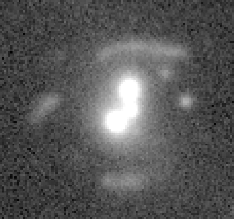
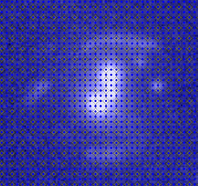
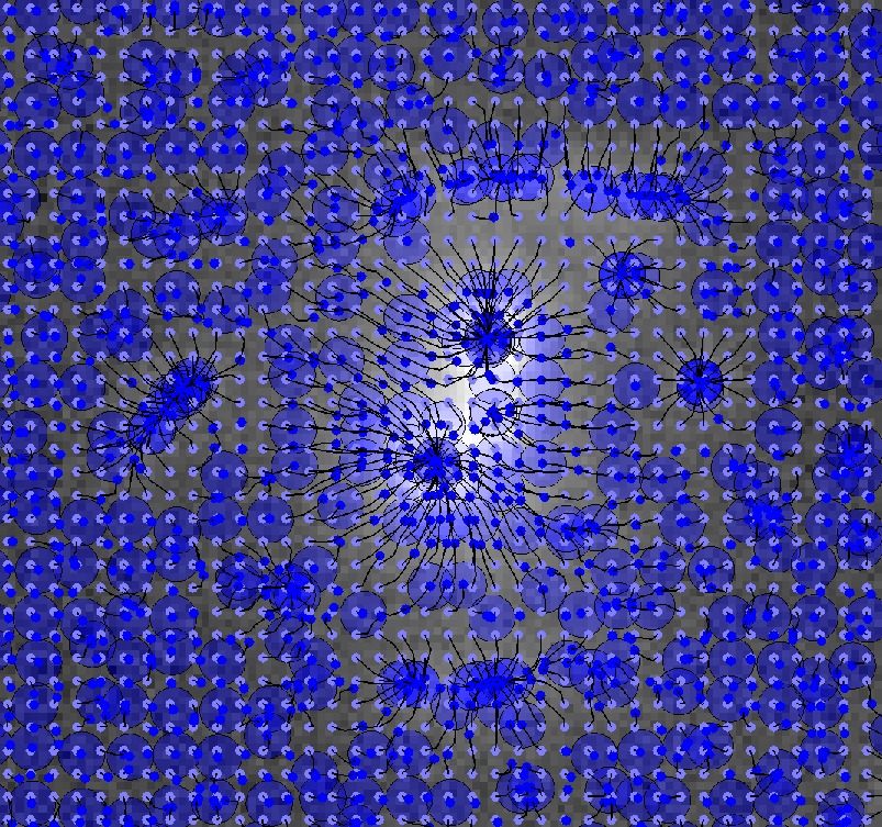
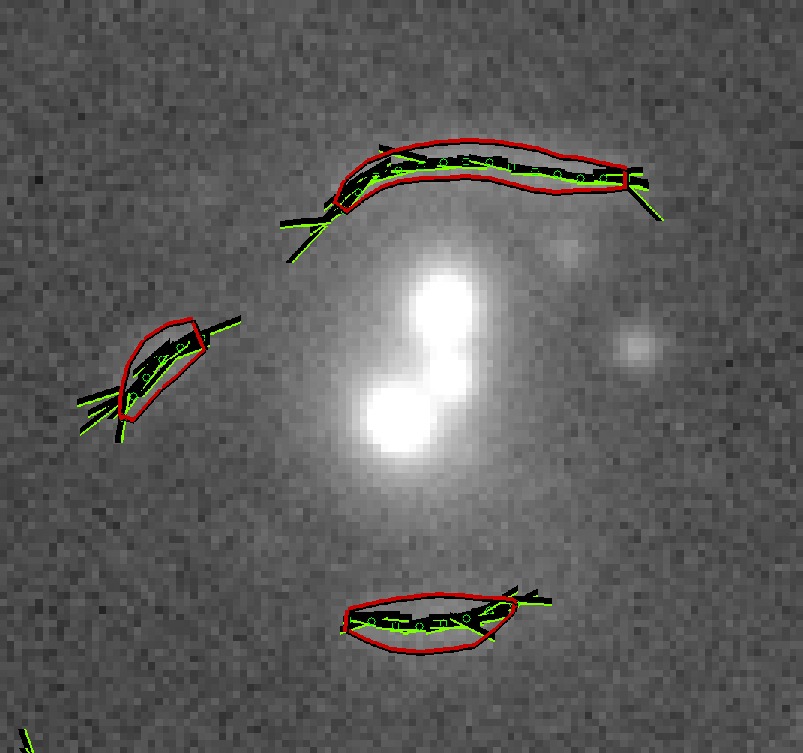
Figure 7: Top-left: I-band SL2S J02140-0535 observation, also featuring a giant arc. Top-right: regular grid of disk shaped areas providing the initial condition of the displacement iterations. Only every second row and column of areas are shown. Bottom-left: areas after three iterations, each moving them to their centre of brightness, and the path they traced. Bottom-right: local orientations for each area, determined using the second brightness moments. Lines corresponding to coherent areas are highlighted. The red contours show the segmentation of the objects.

The arcfinder method tests for coherent orientations in areas preferentially centred on features of locally higher intensity. To achieve this, a regular grid of overlapping, disk shaped areas of equal radii is first placed on the complete image. In three iterations, each area is then displaced to its previous centre of brightness, using a reweighed pixel flux. Areas originally close to a feature move up the slope on both sides, increasing their number density on any significant features’ ridge-lines. On a flat or constantly sloped background, areas only move relative to each other due to pixel noise. At their final positions, each area’s orientation is measured using second moments as described above. To determine coherence, the relative orientations together with the relative placement of areas initially placed close to each other are taken into account. Finally, the centre coordinates of coherent areas are grouped together using a friend-of-friend type algorithm. These groups of coordinates correspond to the initial arcfinder detections.

Filters and post processing

To reduce the number of spurious detections and to expand on the spatial information provided by the area positions and orientations in each detection, filters are applied to the original detections and the shape and flux of each detection are determined. Each of the small detection areas is subjected to a simple fitting procedure that preferentially removes areas centred on point sources and on a background of constant noise without significant structure in the flux distribution. Then, detections with less than a minimal amount of valid areas left or shorter than a threshold are removed. Using a fully automatic active contour evolution method (Kass et al., 1988), isophote contours around each detection are determined, which in turn allows for the determination of the flux. Using the flux and a measurement of the background noise in the larger area surrounding each detection, the signal to noise ratio is set. A more precise length and a length-to-width ratio is computed from the contour, and minimal thresholds are applied to both photometric and morphological data.

Table 5: List of the arcfinder parameters used in this work. For a detailed description refer to the text.

Ridge detection
Gridsize	7	Length and width of each cell [pix]
Cell spacing	0.45	Distance between cells is Cell spacing x Gridsize
Threshold cell	0.45	Coupling threshold for average coupling over the cell neighbourhood
Threshold object	0.75	Coupling threshold for inclusion of a single cell into an object
Threshold graph	0.75	Coupling threshold for graph generation
Filtering
Deblending asymmetry	30	median intensity difference for deblending
Deblending distance	21	minimum deblending distance
Stars saturation intensity	500	critical intensity above which pixels are considered as saturated
Star intensity	50	intensity above which pixels are likely to belong to stars creating diffraction spikes
Star-fluxcoeff spike	3200	compute spike radius as fluxcoeff-spike$\;\times\;{\rm flux}^{1/2}$
Star-fluxcoeff disk	420	compute disk radius as fluxcoeff-disk$\;\times\;{\rm flux}^{1/3}$
Maxpeakflux	0.6	maximal peak flux in ADUs above the background

References

- Bartelmann (2010) Bartelmann, M. 2010, Class. Quantum Grav. 27
- Bartelmann et al. (1998) Bartelmann, M., Huss, A., Colberg, J. M., Jenkins, A., & Pearce, F. R. 1998, A&A, 330, 1
- Bartelmann et al. (1995) Bartelmann, M., Steinmetz, M., & Weiss, A. 1995, A&A, 297, 1
- Bayliss et al. (2011) Bayliss, M. B., Hennawi, J. F., Gladders, M. D., et al. 2011, ApJS, 193, 8
- Benjamin et al. (2007) Benjamin, J., Heymans, C., Semboloni, E., et al. 2007, MNRAS, 381, 702
- Bertin & Arnouts (1996) Bertin, E. & Arnouts, S. 1996, A&AS, 117, 393
- Boulade et al. (2003) Boulade, O., Charlot, X., Abbon, P., et al. 2003, in Society of Photo-Optical Instrumentation Engineers (SPIE) Conference Series, Vol. 4841, Society of Photo-Optical Instrumentation Engineers (SPIE) Conference Series, ed. M. Iye & A. F. M. Moorwood, 72–81
- Bradač et al. (2012) Bradač, M., Vanzella, E., Hall, N., et al. 2012, ApJ, 755, L7
- Broadhurst et al. (2005) Broadhurst, T., Benítez, N., Coe, D., et al. 2005, ApJ, 621, 53
- Cabanac et al. (2007) Cabanac, R. A., Alard, C., Dantel-Fort, M., et al. 2007, A&A, 461, 813
- Clowe et al. (2004) Clowe, D., Gonzalez, A., & Markevitch, M. 2004, ApJ, 604, 596
- Coe et al. (2013) Coe, D., Zitrin, A., Carrasco, M., et al. 2013, ApJ, 762, 32
- Coleman et al. (1980) Coleman, G. D., Wu, C.-C., & Weedman, D. W. 1980, ApJS, 43, 393
- Coles (2008) Coles, J. 2008, ApJ, 679, 17
- Dalal et al. (2004) Dalal, N., Holder, G., & Hennawi, J. F. 2004, ApJ, 609, 50
- de Jong et al. (2012) de Jong, J. T. A., Verdoes Kleijn, G. A., Kuijken, K. H., & Valentijn, E. A. 2012, Experimental Astronomy, 34
- Erben et al. (2009) Erben, T., Hildebrandt, H., Lerchster, M., et al. 2009, A&A, 493, 1197
- Erben et al. (2005) Erben, T., Schirmer, M., Dietrich, J. P., et al. 2005, Astronomische Nachrichten, 326, 432
- Fassnacht et al. (2004) Fassnacht, C. D., Moustakas, L. A., Casertano, S., et al. 2004, ApJ, 600, L155
- Faure et al. (2008) Faure, C., Kneib, J.-P., Covone, G., et al. 2008, ApJS, 176, 19
- Fedeli et al. (2006) Fedeli, C., Meneghetti, M., Bartelmann, M., Dolag, K., & Moscardini, L. 2006, A&A, 447, 419
- Horesh et al. (2005) Horesh, A., Ofek, E. O., Maoz, D., et al. 2005, ApJ, 633, 768
- Ilbert et al. (2009) Ilbert, O., Capak, P., Salvato, M., et al. 2009, ApJ, 690, 1236
- Jackson (2008) Jackson, N. 2008, MNRAS, 389, 1311
- Kass et al. (1988) Kass, M., Witkin, A., & Terzopoulos, D. 1988, International Journal of Computer Vision, 1, 321
- Kneib et al. (2004) Kneib, J.-P., Ellis, R. S., Santos, M. R., & Richard, J. 2004, ApJ, 607, 697
- Kochanek (2006) Kochanek, C. S. 2006, in Saas-Fee Advanced Course 33: Gravitational Lensing: Strong, Weak and Micro, ed. G. Meylan, P. Jetzer, P. North, P. Schneider, C. S. Kochanek, & J. Wambsganss, 91–268
- Laureijs et al. (2011) Laureijs, R., Amiaux, J., Arduini, S., et al. 2011, ArXiv e-prints
- Li et al. (2005) Li, G.-L., Mao, S., Jing, Y. P., et al. 2005, ApJ, 635, 795
- Limousin et al. (2009) Limousin, M., Cabanac, R., Gavazzi, R., et al. 2009, A&A, 502, 445
- Meneghetti et al. (2013) Meneghetti, M., Bartelmann, M., Dahle, H., & Limousin, M. 2013, ArXiv e-prints
- Meneghetti et al. (2003) Meneghetti, M., Bartelmann, M., & Moscardini, L. 2003, MNRAS, 340, 105
- Meneghetti et al. (2000) Meneghetti, M., Bolzonella, M., Bartelmann, M., Moscardini, L., & Tormen, G. 2000, MNRAS, 314, 338
- Merten et al. (2009) Merten, J., Cacciato, M., Meneghetti, M., Mignone, C., & Bartelmann, M. 2009, A&A, 500, 681
- Merten et al. (2011) Merten, J., Coe, D., Dupke, R., et al. 2011, MNRAS, 417, 333
- More et al. (2012) More, A., Cabanac, R., More, S., et al. 2012, ApJ, 749, 38
- Navarro et al. (1997) Navarro, J. F., Frenk, C. S., & White, S. D. M. 1997, ApJ, 490, 493
- Oguri et al. (2012) Oguri, M., Bayliss, M. B., Dahle, H., et al. 2012, MNRAS, 420, 3213
- Richard et al. (2011) Richard, J., Kneib, J.-P., Ebeling, H., et al. 2011, MNRAS, 414, L31
- Richard et al. (2008) Richard, J., Stark, D. P., Ellis, R. S., et al. 2008, ApJ, 685, 705
- Schneider (1999) Schneider, P. 1999, Gravitational lenses
- Seidel & Bartelmann (2007) Seidel, G. & Bartelmann, M. 2007, A&A, 472, 341
- Sheth & Tormen (2002) Sheth, R. K. & Tormen, G. 2002, MNRAS, 329, 61
- Suyu et al. (2010) Suyu, S. H., Marshall, P. J., Auger, M. W., et al. 2010, ApJ, 711, 201
- Tewes et al. (2012) Tewes, M., Courbin, F., Meylan, G., et al. 2012, ArXiv e-prints
- Torri et al. (2004) Torri, E., Meneghetti, M., Bartelmann, M., et al. 2004, MNRAS, 349, 476
- Verdugo et al. (2011) Verdugo, T., Motta, V., Muñoz, R. P., et al. 2011, A&A, 527, A124
- Wambsganss (1998) Wambsganss, J. 1998, Living Reviews in Relativity, 1, 12
- Willmer et al. (2006) Willmer, C. N. A., Faber, S. M., Koo, D. C., et al. 2006, ApJ, 647, 853
- Zacharias et al. (2010) Zacharias, N., Finch, C., Girard, T., et al. 2010, AJ, 139, 2184
- Zitrin & Broadhurst (2009) Zitrin, A. & Broadhurst, T. 2009, ApJ, 703, L132
- Zitrin et al. (2009) Zitrin, A., Broadhurst, T., Umetsu, K., et al. 2009, MNRAS, 396, 1985