Modeling the Resolved Disk Around the Class 0 Protostar L1527

Abstract

We present high-resolution sub/millimeter interferometric imaging of the Class 0 protostar L1527 IRS (IRAS 04368+2557) at $\lambda$ = 870 µm and 3.4 mm from the Submillimeter Array (SMA) and Combined Array for Research in Millimeter Astronomy (CARMA). We detect the signature of an edge-on disk surrounding the protostar with an observed diameter of 180 AU in the sub/millimeter images. The mass of the disk is estimated to be 0.007 $M_{\sun}$, assuming optically thin, isothermal dust emission. The millimeter spectral index is observed to be quite shallow at all the spatial scales probed; $\alpha$ $\sim$ 2, implying a dust opacity spectral index $\beta$ $\sim$ 0. We model the emission from the disk and surrounding envelope using Monte Carlo radiative transfer codes, simultaneously fitting the sub/millimeter visibility amplitudes, sub/millimeter images, resolved L′ image, spectral energy distribution, and mid-infrared spectrum. The best fitting model has a disk radius of R = 125 AU, is highly flared ($H$ $\propto$ $R^{1.3}$), has a radial density profile $\rho$ $\propto$ $R^{-2.5}$, and has a mass of 0.0075 $M_{\sun}$. The scale height at 100 AU is 48 AU, about a factor of two greater than vertical hydrostatic equilibrium. The resolved millimeter observations indicate that disks may grow rapidly throughout the Class 0 phase. The mass and radius of the young disk around L1527 is comparable to disks around pre-main sequence stars; however, the disk is considerably more vertically extended, possibly due to a combination of lower protostellar mass, infall onto the disk upper layers, and little settling of $\sim$1 µm-sized dust grains.

1 Introduction

In the earliest stages of star formation, the Class 0/I phases (Andre et al., 1993; Lada, 1987), a newborn protostar is embedded within a dense infalling envelope of gas and dust. Disks are thought to naturally form in these systems due to conservation of angular momentum in the collapsing cloud; several analytic models have been developed that explain the formation of disks within infalling envelopes (Cassen & Moosman, 1981; Terebey et al., 1984). Observational characterization of disks around Class 0/I objects has been difficult because emission from the surrounding envelope is entangled with that of the disk (e.g. Chiang et al., 2008; Jørgensen et al., 2009). However, the disks around more evolved young stars without envelopes, Class II sources, have been studied in great detail in recent years, deriving their surface density distributions, radii, masses, and dust opacity spectral indicies from sub/millimeter interferometric imaging (e.g. Dutrey et al., 1996; Kitamura et al., 2002; Andrews et al., 2009; Isella et al., 2009; Ricci et al., 2010; Kwon et al., 2011). Gaps and holes have also been discovered in disks around pre-main sequence stars (Calvet et al., 2005; Piétu et al., 2006; Espaillat et al., 2007, 2008; Hughes et al., 2009), which are interpreted as signs of planets formation, suggesting that disks are ultimately cleared by the accretion of material onto proto-planets.

A relatively clear picture of pre-main sequence disk properties and how disks are dispersed has been gained; however, we still do not have a clear observational picture of how the life of a disk begins. Large disks have been clearly shown to exist in the Class I phase (Eisner, 2012; Wolf et al., 2008; Padgett et al., 1999; Launhardt et al., 2001; Jørgensen et al., 2009; Takakuwa et al., 2012; Eisner, 2012), but firm detections of Class 0 protostellar disks have remained elusive (Looney et al., 2003; Harvey et al., 2003; Jørgensen et al., 2009; Chiang et al., 2008, 2012) and a controversy exists as to their expected properties. Specifically, it has remained uncertain whether or not large disks form during this phase and their expected masses.

Hydrodynamic simulations show that disks can grow to large radii rather quickly in the absence of strong magnetic fields (Yorke & Bodenheimer, 1999) and are are often massive enough to fragment (Vorobyov, 2010). On the other hand, Models of protostellar collapse in magnetized envelopes have difficulty forming rotationally supported disks under the assumption of ideal magneto-hydrodynamics (MHD) due to strong magnetic braking as field lines are dragged inward, this is the so-called ”magnetic braking catastrophe” (e.g. Allen et al., 2003; Galli et al., 2006; Hennebelle & Fromang, 2008; Mellon & Li, 2008). Recently models that consider non-ideal MHD have been able to form small, rotationally-supported disks as the magnetic flux is dissipated via Ambipolar Diffusion and Ohmic dissipation (Dapp & Basu, 2010; Machida et al., 2010). Disks in these simulations are expected to have radii $<$ 100 AU until the end of the Class I phase; however, the robustness of Ohmic dissipation for the formation of rotationally-supported disks has been questioned (Li et al., 2011). Nonetheless, simulations considering non-idealized initial conditions (i.e. magnetic field mis-alignment with rotation axis and turbulent cores) are able to form rotationally supported disks under the assumption of ideal MHD (Joos et al., 2012; Seifried et al., 2012).

Despite the large body of theoretical and numerical work toward understanding disk formation, only a few Class 0/I systems have been observed with sufficient resolution and sensitivity in the millimeter spectral range to even have the possibility of characterizing the properties of disks in this early phase of evolution. A modest resolution protostellar survey with the Sub-millimeter Array (SMA) by Jørgensen et al. (2009) found that the compact dust continuum emission from protostars is consistent with the presence of disks having masses between 0.002 and 0.5 $M_{\sun}$. However, modeling of millimeter continuum data from Class 0 protostars indicates that non-uniform density structure (i.e. radial density enhancements at small-scales) can reproduce the observed data without a disk (Chiang et al., 2008). Maury et al. (2010) carried out a high-resolution study toward five protostars in Taurus and Perseus with the Plateau de Bure Interferometer (PdBI) and did not detect disks or close binaries. The authors then argued that the formation of large disks and fragmentation are suppressed by magnetic fields during collapse.

Contrary to theoretical expectations, a clear detection of a Class 0 disk is found toward the protostar L1527 in Taurus (d=140 pc) (Tobin et al., 2010a, 2012, hereafter Papers I & II). Paper I presented high resolution L^′-band (3.8$\mu$m) observations of L1527 and found the apparent signature of an edge-on protostellar disk in near-infrared scattered light. Follow-up observations with the SMA and Combined Array for Research in Millimeter-wave Astronomy (CARMA) at $\sim$0$\farcs$3 resolution found the dust emission to be resolved and elongated in the same direction as the near-infrared dark lane (Tobin et al., 2012). Moreover, $\sim$1″ resolution observations of the ¹³CO detected the signature of Keplerian rotation in the disk via spectro-astrometry, enabling the protostellar mass to be constrained to be 0.19$\pm$0.04 $M_{\sun}$.

In this paper, we present radiative transfer modeling of the disk around L1527. We attempt to construct a realistic model of the protostellar disk embedded within its envelope by simultaneously considering the disk continuum emission, multi-wavelength SED, Spitzer IRS spectrum, and L′ image. We find that the data are best reproduced by a highly-flared R = 125 AU, M = 0.0075 $M_{\sun}$ disk, with a very shallow dust emissivity spectral index. Section 2 describes our observations and data reduction, our observational results are presented in Section 3, we discuss the modeling in Section 4, the results are discussed in Section 5, and conclusions are given in Section 6.

2 Observations and Data Reduction

The observations we present are among the highest resolution taken toward a Class 0 protostar using CARMA (Woody et al., 2004) at $\lambda$ = 3.4 mm and the SMA (Ho et al., 2004) at $\lambda$ = 870 µm. The data were taken in multiple configurations at both facilities, gaining sensitivity to both large and small-scale structures in the protostellar envelope and disk.

2.1 CARMA Observations and Data Reduction

The CARMA 3.4 mm data were taken in all five CARMA configurations between 2008 and 2010. We discuss the A and B array data separately from the C, D, and E-array observations due to the different calibration techniques. Details of each observation are given in Table 1.

2.1.1 3.4 mm A & B-array

The A-array observations of L1527 were taken on 2010 December 02 during stable conditions with $\sim$4mm of precipitable water vapor (pwv). The local oscillator was tuned to $\nu$=90.7510 GHz and the correlator was configured for 4-bit sampling with 8 - 500 MHz moveable spectral windows, measuring continuum emission. The IF range spans 1 to 9 GHz and we arranged windows such that they occupied the 1 to 5 GHz range of IF bandwidth. The receivers operate in dual-sideband (DSB) mode and the full instantaneous bandwidth was 8 GHz in one polarization. The primary gain calibrator was 3C111, 12.8 degrees away on the sky; 0431+206 was observed as a test source in conjunction with L1527. 3C84 was observed as the bandpass calibrator, and Neptune was observed as the absolute flux calibrator. The observations were conducted in a standard loop, observing 3C111 for 3 minutes, L1527 for 7 minutes, 0431+206 for 1 minute, and then repeating. Pointing was updated periodically using optical pointing correction and radio pointing was done once during the track.

The B-array observations were taken on 2010 January 02 and 06. The local oscillator was tuned to $\nu$=87.27 GHz during both observations and one 500 MHz spectral window was configured for continuum observation. This yielded 1 GHz of total continuum bandwidth in DSB, with the windows centered on $\nu$=85.5 and 89.05 GHz. These observations were taken using the old correlator with less overall bandwidth. The primary gain calibrator was 3C111, 3C123 was observed as test source, 3C84 was the bandpass calibrator, and Uranus was observed as the flux calibrator in the first track. No flux calibrator was observed during the second track, so the flux of 3C111 was carried over from the first track because they were observed only 4 days apart. The observations were conducted in a loop, observing 3C111 for 3 minutes, L1527 for 9 minutes, and 3C123 for 3 minutes.

The CARMA paired antenna calibration system (C-PACS) was used for enhanced atmospheric phase correction in both the A and B-array observations. Briefly, the C-PACS calibration works as follows, the eight 3.5 meter dishes from the SZ array are positioned next to the 10.4 meter and 6 meter antennas at the longest baselines. While the source(s) is being observed, the 3.5 meter dishes are observing a nearby calibrator at 30 GHz. The short timescale phase variations during the observation of the source(s) are corrected from the simultaneous calibrator observations by the 3.5 meter antennas. This correction effectively reduces the atmospheric decorrelation at the longest baselines, so long as the C-PACS calibrator is sufficiently close to the source(s). A more detailed explanation of the C-PACS system is given in Pérez et al. (2010). During the A-array observation of L1527, the C-PACS antennas observed the quasar 0428+329 (7.4° away) with a flux density of 1.9 Jy at 30 GHz. For the B-array observations, the C-PACS antennas observed the quasar J0403+260 (8.3° away) and had a flux density of 1.6 Jy.

2.1.2 3.4 mm C, D, & E-array Observations

The C-array observations were conducted on 2009 May 28 and 2009 October 11. The local oscillator was tuned to $\nu$=87.27 GHz and two 500 MHz bands were configured for continuum observation (2GHz DSB). 3C111 was observed as the gain calibrator, 3C84 and Uranus were the flux calibrators, and 0423-013 and 3C84 were the bandpass calibrators. L1527 was again observed in D-array on 2009 July 28 and 30, as well as 2008 August 31 with the local oscillator tuned to $\nu$=87.27 GHz for the 2009 July observations and $\nu$=91.2 GHz for the 2008 August observations. In both data sets, two 500 MHz bands were configured for continuum observation (2GHz DSB). 3C111 was observed as the gain calibrator, Uranus and Mars were the flux calibrators, and 3C111 and 3C84 were the bandpass calibrators. Lastly, L1527 was observed in E configuration in 2008 October; these observations were taken in a three-point mosaic to better recover the large-scale emission from the envelope. The correlator was configured with one band for 500 MHz continuum, the other two bands were set to observe N₂H⁺ ($J=1\rightarrow 0$) and HCO⁺ ($J=1\rightarrow 0$). The N₂H⁺ and E-array continuum observations were previously presented in Tobin et al. (2011). 3C111 was observed as the gain calibrator and 3C84 was observed as both the flux and bandpass calibrator.

2.1.3 Data Reduction

The data were reduced using the MIRIAD software package (Sault et al., 1995). The visibilities were first corrected for the updated baseline solutions and transmission line length correction. Then the amplitudes and phases were examined for each baseline, flagging the source observations between points where the calibrator had bad amplitudes or extremely high phase variance. The data were then bandpass corrected using the mfcal task. The absolute flux calibration was calculated using the bootflux task to determine the flux of 3C111 relative to the absolute flux calibrator. We compared the visibility amplitudes of L1527 in ranges of overlapping uv-coverage to estimate our flux calibration uncertainty. There was excellent agreement between the 3.4 mm datasets and we estimate an absolute flux uncertainty of $\sim$10%.

For the A and B-array data taken with the C-PACS system, the 30 GHz data were also inspected for bad amplitudes and phases. One C-PACS antenna was offline during the A-array track, but all eight were operational for the B-array tracks. The C-PACS data were bandpass corrected using 3C111 and the data were self-calibrated on a timescale of 4 seconds. The time-dependent phase correction to apply to the science data was calculated by the gpbuddy task and the corrections were applied using the uvcal task with the atmcal option. The science array gain calibrations were then calculated for 3C111 with the mselfcal task and this solution was applied to the observations of L1527. The angular separation of the C-PACS calibrator to L1527 was not ideal but, the correction did reduce the root-mean squared (RMS) phase scatter on 3C111 from $\sim$60° to $\sim$40°, comparable effectiveness is assumed on the L1527 observations.

The data were then imaged by first computing the inverse Fourier transform of the data with the invert task, weighting by system temperature and creating the dirty map. The dirty map is then CLEANed using the mossdi task and the image is restored and convolved with the CLEAN beam by the restor task. The images were cleaned down to 1.5$\times$ the RMS. The images of the test sources 0431+206 and 3C123 were also reconstructed to ensure that these secondary calibrators appear as point sources as a check of the millimeter “seeing”. The test source images were point sources, confirming the good conditions.

2.2 Submillimeter Array Observations

We observed L1527 with the Submillimeter Array (SMA) at Mauna Kea on 2011 January 5 and 6. The data were taken in very extended configuration with 7 antennas operating. The first track had excellent phase coherence but the pwv was $\sim$4.0 mm and the second track had $\sim$2.0 mm pwv, but worse phase coherence. The local oscillator was tuned to $\nu$=347.02 GHz and the correlator was used in 4 GHz (DSB) mode. The correlator was configured for 32 channels per chunk, the coarsest resolution mode for continuum observations, each chunk is 104 MHz wide and there are 48 correlator chunks. The IF frequency was chosen to overlap with the compact array dataset taken by the PROSAC project on 2004 December 17 (Jørgensen et al., 2007). 3C111 was observed as the gain calibrator, 0510+180 was observed as a secondary calibrator, 3C279 was the bandpass calibrator, and Callisto was the absolute flux calibrator. The data were taken in the following loop: 3C111 was observed for 2.5 minutes, then L1527 was observed for 8 minutes, then 0510+180 was observed for 2.5 minutes, then L1527 again and finishing with 3C111.

The compact array observations were taken on 2004 December 18 and reported in Jørgensen et al. (2007). Seven antennas were operating during the track; however, only six antennas produced useable data. The correlator had three chunks configured for higher resolution spectral line observations and the rest configured for continuum measurement; including the spectral line chunks with more channels, the observations had 2 GHz (DSB) of bandwidth. The gain calibrators were 3C111 and 0510+180, Saturn was used for bandpass calibration, and the flux calibrator was Uranus. The data were taken observing 3C111 for 5 minutes, L1527 for 15 minutes, and 0510+180 for 5 minutes, then L1527 again and repeating the cycle. Details of the observations are given in Table 2.

The data were reduced using the MIR software package, an IDL-based software package originally developed for the Owens Valley Radio Observatory and adapted by the SMA group. The data were first corrected for the updated baseline solutions and then phases and amplitudes on each baseline were inspected and uncalibrateable data were flagged. The system temperature correction was then applied to the data and the bandpass correction was calculated, trimming three channels at the edge of each correlator chunk. After bandpass calibration, a first-pass gain calibration was performed on 3C111, 0510+180, and Callisto to measure the calibrator fluxes. The L1527 and 0510+180 data were then calibrated for amplitude and phase using only 3C111. The visibility amplitudes of the compact and very extended configuration data were consistent in the regions of uv overlap, despite the different flux calibrators; we estimate an absolute flux uncertainty of 10%. The data were then exported to MIRIAD format for imaging and were imaged using the same technique as outlined in the previous section. 0510+180 was additionally imaged and found to be a point source, confirming the excellent submillimeter seeing conditions for the very extended observations.

3 Results

The observations of L1527 at multiple wavelengths and configurations enable us to perform a broad observational characterization of the dust continuum emission from the protostar. We compare and combine our work with previous observations of L1527 taken with Gemini, PdBI, VLA, and EVLA to derive a more complete understanding of the disk and envelope.

3.1 Multi-Configuration Images

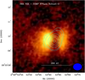
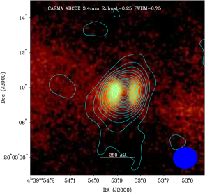
Figure 1: Images of L1527 from the SMA at 870 µm (left) and CARMA at 3.4 mm (right) including data from all observed array configurations. The addition of shorter-spacing data enable larger scale emission to be recovered. The larger-scale emission is more extended in the direction of the dark lane. The SMA data are extended in the vertical direction, coincident with the brighter lobe of the scattered light, possibly indicative of additional heating. For the SMA data, the contours start at $\pm$2$\sigma$, 3$\sigma$ and increase in units of 3$\sigma$. For the CARMA data, the contours start at $\pm$3$\sigma$ and increase by 3$\sigma$ until 15$\sigma$ where they increase by 5$\sigma$. The RMS noise level ($\sigma$) in the 870 µm data is 11 mJy beam^-1 and 0.29 mJy beam^-1 in the 3.4 mm data.

The observations of L1527 in multiple configurations enable the physical structure of the envelope and disk to be examined at multiple spatial scales. In addition to the most extended configurations, data have also been taken for L1527 in more compact configurations at both the SMA and CARMA. The resultant images are shown in Figure 1, overlaid on the L′ image of the edge-on scattered light structure from Tobin et al. (2008). The combined datasets trace larger-scale structures, but emphasize different features. The CARMA 3.4 mm data have extended emission on $\sim$4″ scales that could be tracing the extended disk structure or a rotationally-flattened inner envelope meeting the disk. The SMA image remains more compact, but trace smaller-scale extended emission in the same direction as the CARMA large-scale emission; a difference is that the SMA data appear more extended along the vertical direction of the disk, coincident with the brighter scattered light feature. The SMA data does not recover larger-scale emission due to a lack of shorter uv-spacings and a more sparsely sampled uv-plane. The measured flux densities from these multi-configuration data are given in Table 3.

3.2 High-resolution Images and Disk Size

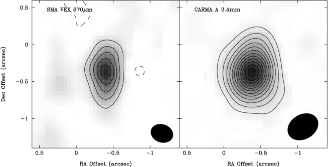
Figure 2: High-resolution continuum images for L1527 from the SMA at 870 µm (left) and CARMA at 3.4 mm (right), both use natural weighting. The contours in all images start at 3$\sigma$ and increase in 3$\sigma$ intervals; $\sigma$ = 5.0 mJy beam^-1 (SMA), and 0.24 mJy beam^-1 (CARMA 3.4 mm). Both the 870 µm and 3.4 mm data are extended normal to the outflow direction and in the same direction as the dark lane imaged with Gemini at L′-band. These data are consistent with L1527 harboring an edge-on disk.

The naturally-weighted image from the SMA very extended data is shown in the left panel of Figure 2. The image shows dust emission extended in the direction of the dark lane imaged by Gemini, subtending $\sim$1$\farcs$0 in diameter. The CARMA A-array 3.4 mm image, also generated using natural-weighting, is shown in the right panel. In contrast to the SMA image, the central point source is more prominent, but there is extension in the same direction and with similar angular extent as the SMA data. These datasets are both tracing the embedded protostellar disk around L1527 and are qualitatively similar to other observations of edge-on disks surrounding more evolved sources (e.g. Wolf et al., 2008).

Since these observations resolve the protostellar disk, one of the key parameters to measure is its size. From the very extended and A-array data alone, the disk size is measured to be $\sim$0$\farcs$95$\times$0$\farcs$55 ($\sim$133$\times$77 AU $\pm$ 19 AU) and $\sim$1$\farcs$15$\times$0$\farcs$85 ($\sim$160$\times$120 AU $\pm$ 12 AU) in the SMA and CARMA images respectively. The size was determined by measuring the maximum dimension enclosed by the 3$\sigma$ contour along the long and short axis of emission in the convolved image. The size of the short axis of the disk will be over estimated due to convolution with the beam; however, the major axis length is resolved in both images. The full width at half maxima (FWHM) from fitting the images with a two dimensional Gaussian are approximately half the length measured inside the 3$\sigma$ contour. The deconvolved FWHM are comparable to the FWHM of the Gaussian along the major axis, but the deconvolved sizes of the minor axes are about a factor of two smaller than the fit. Values for the Gaussian fits are given in Table 3.

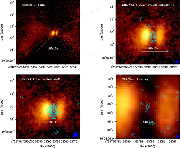
Figure 3: L^′ image of L1527 with millimeter continuum data overlaid on the sub-panels. Top Left: L^′ image of L1527 showing the full range of the high-resolution Gemini data. Top Right: Zoom-in on the L^′ image with SMA 870 µm data overlaid on the L^′ image. Bottom Left: CARMA 3.4 mm data overlaid on the zoomed image. Bottom Right: Further zoom-in on the L^′ data with VLA 7mm data from Loinard et al. (2002) overlaid. Note that the millimeter data were manually centered on the dark lane as the registration of the L^′ image is approximate. The contours in all images start at 3$\sigma$ and increase in 3$\sigma$ intervals; $\sigma$ = 5.0 mJy beam^-1 (SMA), 0.24 mJy beam^-1 (CARMA 3.4 mm), 0.3 mJy beam^-1 VLA.

The millimeter images are overlaid on the L′ image from Paper I in Figure 3. The radius of disk inferred from the millimeter emission is $\sim$ 2x smaller than what was determined from modeling in Paper I. However, the smaller region of resolved millimeter emission is not inconsistent with a larger disk being present as the emission may simply be too faint to detect and/or be resolved-out at these large radii. The 7 mm VLA A-array image from Loinard et al. (2002) is also included in this plot, showing the small-scale emission from the inner disk; these data are clearly missing substantial larger-scale flux from the disk due to lack of shorter uv-spacings and/or sensitivity.

3.3 Visibility Data

We examine the flux density versus uv-distance in Figure 4. The visibilities amplitudes from all observed array configurations in the two wavelengths bands are shown in the individual subpanels. Between uv-distances of 0 to $\sim$200 k$\lambda$ the amplitude vs. uv-distance trend is similar at all wavelengths; however, at uv-distances longward of 300 k$\lambda$ the CARMA 3.4 mm visibilities flatten out. At these uv-distances the SMA data are continuing a downward trend, but are still above the noise floor. The differences between the CARMA and SMA visibilities indicate that the 3.4 mm data have an additional unresolved component to the flux that is not present or substantially weaker at 870 µm. Flat visibility curves at long baselines in protostellar objects have previously been used to infer the presence of an unresolved disk (e.g. Harvey et al., 2003). However, if we are examining dust emission from the same structure at both 870 µm and 3.4 mm, then the visibility curves should be nearly identical.

The most likely culprit for the unresolved emission is the thermal jet, radiating free-free emission. Reipurth et al. (2002) observed L1527 with the VLA in A-configuration at 3.6 cm (0$\farcs$3 resolution), detecting a point source and Melis et al. (2011) conducted new observations with the EVLA between 7 mm and 6 cm finding that S_λ(ff) $\propto$ $\lambda^{-0.33}$. Extrapolating this slope to 3.4 mm, the free-free contribution to the continuum flux is expected to be 1.76 mJy, consistent with the visibility amplitudes measured at baselines $>$300 k$\lambda$. Thus, the free-free jet emission is contaminating the dust continuum emission at 3.4 mm. Its removal from the data is trivial since the emission is point-like. We subtracted the 1.76 mJy point source from all 3.4 mm datasets using the MIRIAD task uvmodel centered on the continuum peak position at 3.4 mm.

The visibility plot from the subtracted dataset is shown in Figure 4. The flux densities measured from the CARMA (free-free corrected) 3.4 mm A-array and SMA 870 µm very extended images are given in Table 3. With the corrected data, we can clearly show that the observations toward L1527 do not show the flat visibilities at long baselines, due to the extended nature of the disk and emission being resolved across all observed uv-distances.

3.4 Millimeter SED

In the millimeter regime, if the dust temperature is isothermal and optically thin, the spectral index of thermal dust emission should follow the relation

$$F_{\lambda}\propto F_{\lambda,0}\left(\frac{\lambda_{0}}{\lambda}\right)^{\alpha},$$ (1)

with $\alpha$ = 2 + $\beta$, assuming the Rayleigh-Jeans limit, and $\beta$ is the dust opacity spectral index. Therefore, if the emission is optically thin and isothermal we can calculate $\beta$ directly from the sub/millimeter flux densities. The flux densities measured at CARMA A-array and SMA very extended array yield $\alpha$ $\sim$ 1.9, implying $\beta$ $\sim$ 0. We plot our observed fluxes at 870 µm and 3.4 mm along with 1.3 mm fluxes from Maury et al. (2010) and the 7 mm to 6 cm fluxes observed by Melis et al. (2011) in Figure 5. All these data are consistent with $\alpha$ = 2 and $\beta$ = 0, given the assumptions of isothermal and optically thin emission. In the absence of large flux calibration offsets, this result could indicate the following: the emission is becoming optically thick, the dust is not isothermal, and/or a gray opacity law in the millimeter. A gray opacity would result if the dust grains probed by these observations were larger than the observed wavelength. However, Melis et al. (2011) suggested that their 1.3 cm data indicated a lack of cm-sized grains, but Scaife et al. (2012) used a different fitting method and had more cm-wave data that indicated a presence of cm-sized grains, see section 5 for further discussion.

We have examined the spectral index of the visibility amplitudes versus uv-distance in Figure 6 (using the free-free corrected data at 3.4 mm). Across the overlapping uv-range the emission is consistent with $\alpha$ = 2 at both large (envelope; 1000s of AU) and small (disk; 100s of AU) spatial scales. A caveat here could be that the flux densities are only accurate to $\sim$10% at best, which yields an uncertainty in $\beta$ of $\sim$0.1 (Chiang et al., 2012); for 20% errors in flux calibration the uncertainty increases to 0.21. Therefore, even with large amplitude calibration errors the shallow spectral index of the disk appears to be real. A shallow opacity spectral index is not necessarily unexpected given that Taurus Class II sources also often consistent with $\beta$ $\sim$ 0 using optically thin assumptions (Andrews & Williams, 2005; Ricci et al., 2010). In addition, Kwon et al. (2009) found shallow $\beta$ values (0.5 - 1.0) in protostellar envelopes on 1000s of AU scales.

3.5 Disk Mass

The disk mass can be simplistically calculated using the same assumptions of isothermal and optically thin dust emission as we used to determine the spectral index. We assume a dust opacity law normalized to $\kappa_{0}$=3.5 cm² g^-1 (dust only) at 850µm(Andrews & Williams, 2005), a dust-to-gas mass ratio of 1:100, and the observed dust opacity spectral index ($\beta$) = 0. We then calculate the mass assuming optically thin emission and constant dust temperature with the following equation

$$M_{dust}=\frac{D^{2}F_{\lambda}}{\kappa_{0}\left(\frac{\lambda}{850\mu m}\right)^{\beta}B_{\lambda}(T_{dust})},$$ (2)

where $D$ = 140 pc and $T_{dust}$ is estimated to be 30K. The flux densities at 870 $\mu$m and 3.4 mm were taken from Table 3, using the SMA very extended and CARMA A-array measurements. This yields mass estimates of 0.007 and 0.007 $M_{\sun}$ at 3.4 mm and 870 µm respectively, with a statistical uncertainty of $\pm$ 0.0007 $M_{\sun}$. If we had not assumed $\beta$ = 0, and chosen $\beta$ = 1 as is typically done (Andrews & Williams, 2005; Andrews et al., 2009), then there would be a factor of $\sim$3 discrepancy in the mass calculated at different wavelengths. The possible reasons for such a shallow $\beta$ in this source are further discussed in Section 5.

4 Modeling

To better understand the physical properties of the disk around L1527, we model the thermal dust emission in the sub/millimeter, L′ image, and multi-wavelength SED. We use the Monte Carlo radiative transfer code of Whitney et al. (2003) to calculate the propagation of radiation through the disk and envelope, determining the spectral energy distribution (SED) from the near-infrared to the millimeter, producing scattered light and thermal images in the near to far-infrared; external heating is also considered by the standard interstellar radiation field extincted by A_V = 3. We use the envelope density structure from the rotating collapse model (Ulrich, 1976; Cassen & Moosman, 1981; Terebey et al., 1984, hereafter CMU model). This density structure is spherical at large radii, but near the centrifugal radius ($R_{C}$) the envelope becomes flattened due to rotation; the envelope density scaling is linked to the mass infall rate. Outflow cavities are also included in this modeling with the same parameters as in Paper I. The density structure of the disk is defined by a radial density profile, flaring as a function of disk radius, Gaussian vertical density profile, an initial scale height, and total mass.

We have run a grid of models, keeping the envelope properties constant, while varying the properties of the circumstellar disk (radius, flaring, radial density profile, scale height, and mass). The central protostellar mass is assumed to be 0.5 $M_{\sun}$; however, no parameters directly depend on this value. The protostar mass is only used to calculate the disk-protostar accretion luminosity and convert the envelope mass infall rate into the envelope density of the CMU model. The mass infall rate is taken to be 1.0 $\times$ 10^-5 $M_{\sun}$ yr^-1, identical to Tobin et al. (2008), but 25% larger than that used in Paper I. We also assume the same disk-protostar accretion rate, yielding L_acc=1.75 $L_{\sun}$ and a protostellar luminosity of 1.0 $L_{\sun}$. Note that the measured protostellar mass of 0.19 $M_{\sun}$ suggests that the luminosity of the protostar may be lower and the accretion luminosity would be greater; however the source of emission will not significantly alter the sub/millimeter emission. Table 4 gives a complete list of model parameters and identifies those varied or fixed. The total number of models run was 3,584, using five free parameters.

The key constraints on the disk properties for L1527 lie in the high-resolution sub/millimeter and L′ images. The Whitney et al. (2003) code can produce images at these wavelengths; however, the images are constructed from the individual photons that are either absorbed/reemitted or scattered on their way out of the envelope. This imaging method works well for scattered light at L′-band and other wavelengths where there is substantial flux, but an impractical number of input photons are needed to produce reasonable high-resolution sub/millimeter images. Therefore, to generate high-resolution sub/millimeter images with high-signal to noise, we use the temperature and density structure calculated by the Whitney et al. (2003) code as input to the LIME (LIne Modeling Engine) radiative transfer code (Brinch & Hogerheijde, 2010), using the ray-tracing function to generate dust continuum images. The MIRIAD task uvmodel is used to calculate the Fourier transform of the model image and sample it with the same uv-coverage as the CARMA and SMA observations. We then use the uvamp task to calculate the flux versus projected baseline for a given model in circularly averaged bins of uv-distance identical, to those in Figure 4. Note that while the uv-coverage is identical, the effects of atmospheric decorrelation and thermal noise are not taken into account for the model visibilities.

4.1 Dust Opacities

The dust model used for the envelope and disk with the Whitney et al. (2003) code is the same as presented in Tobin et al. (2008), with grains up to $\sim$1 µm in radius and an assumed mixture of discrete spherical grains composed of graphite, astronomical silicates, and water ice. The dust opacity spectral index ($\beta$) of this model at sub/millimeter wavelengths is 1.93; ISM dust grains have $\beta$ $\sim$ 2 for comparison. However, we found that these dust opacities were found to be too low (0.6 cm² g^-1 at 870 µm; opacity of dust only) at sub/millimeter wavelengths. Moreover, the spectral index of these opacities is much steeper than found in the observations, 1.93 versus $\sim$0. Therefore, models of dust emission using the same opacities from the radiative equilibrium code cannot simultaneously reproduce the emission at both 870 µm and 3.4 mm. It is possible that the disk is simply very massive and optical depth effects are causing the the shallow observed spectral index; however, then the disk would be too opaque to reproduce the L′ scattered light structure. We also cannot simply use larger-grain models in the radiative equilibrium calculation because that makes the SED fit bad from $\sim$3 µm to 70 µm, due to the sensitivity of the mid-infrared SED shape to the maximum grain size.

A dust model with maximum grain sizes between $\sim$1 to 10 cm and a shallow power-law size distribution $N(a)$ $\propto$ $a^{-2.5}$ - $a^{-3.0}$ could reproduce the observed spectral index from 870 µm to 3.4 mm (D’Alessio et al., 2001; Hartmann, 2008; Ricci et al., 2010) and Scaife et al. (2012) indicated that there was evidence for cm-sized grains in L1527. Given these uncertainties, we chose to adopt a parametrized sub/millimeter dust opacity in the LIME raytracing calculation to simplify modeling because a detailed exploration of dust opacities is beyond the scope of this study. Other published studies (e.g. Looney et al., 2003; Chiang et al., 2012) have adopted similarly parametrized sub/millimeter dust properties, deviating from the dust opacity model used at shorter wavelengths in the radiative transfer calculation. The need to adopt a parametrized dust opacity at sub/millimeter wavelengths reflects the inability of dust models to fully describe the opacities across all wavelengths with a single self-consistently generated model or spatial variation in the dust size distribution.

We normalized the sub/millimeter dust opacity at 850 µm to be of 3.5 cm² g^-1 (Andrews & Williams, 2005) and varied the spectral index between 0.0 and 0.75 in steps of 0.25. The use of a different opacity in the millimeter should not impact the calculated dust temperature structure, because most energy is absorbed by the dust grains at wavelengths shortward of 100 µm. The small values of the dust opacity spectral index modeled are motivated by the shallow spectral index from 3.4 mm to 870 µm and that other millimeter studies of protostars often find values of $\beta$ $\lesssim$ 1 (Kwon et al., 2009; Chiang et al., 2012). Including these dust opacity variations, the total number of models increases to 14,336.

4.2 Model Fitting

The large number of models generated with combinations of the five parameters explored necessitates using statistical tests to weed out the large fraction of models that do not fit the data. To do this, we simultaneously fit the 870 µm and 3.4 mm visibilities, sub/millimeter images, the multiwavelength SED, and IRS spectrum by calculating individual $\chi^{2}$ values for each type of data and computing the average.

We calculate the $\chi^{2}$ of the azimuthally averaged model visibilities at 870 µm, and 3.4 mm using the equation

$$\chi^{2}=\sum_{i}^{N}\frac{(F_{\nu,observed,i}-F_{\nu,model,i})^{2}}{\sigma_{i}^{2}}$$ (3)

for the nine visibility points between 0 and 400 k$\lambda$ taken in 50 k$\lambda$ bins, as shown in Figure 4. The uncertainty in the data, $\sigma_{i}$, includes the statistical uncertainty in addition to a 5% absolute flux uncertainty; although the true absolute flux uncertainty for these data is $\sim$10%, we could not assign such an uncertainty to each point without making many models appear overly well-constrained. This is because the absolute flux uncertainty is an overall offset in the scaling of the flux densities and not random noise. Also note that once the signal to noise of the visibility data in a given bin is less than $\sim$3, the errors are no longer Gaussian but follow the Rice distribution. We do not expect this to significantly affect our fitting as the lowest signal-to-noise is 3.7 for one point in the CARMA 3.4 mm data; outside our chosen range for fitting the visibilities do have signal-to-noises less than 3.

We calculate the $\chi^{2}$ of the spectral energy distribution from the near-infrared to the millimeter, in a similar manner to equation 3; this to ensures that the models fitting the millimeter visibilities also result in a reasonable SED. The IRS spectrum is also fit from 11 $\micron$ to 20.7 µm. We select a subset of the full IRS spectral range in order to avoid ice features present between 6 µm and 11 µm as well as the wings of the 45 µm water ice feature apparent at the long wavelength end of the IRS spectrum.

Since the azimuthally averaged visibilities do not contain information about the two-dimensional structure of the source, we also use the sub/millimeter images as a constraint on the resolved disk structure. We directly compare the models to the data by subtracting the model visibilities from the data and then reconstructing the images from the residual uv dataset. We only use the highest resolution dataset (A-array for CARMA and very extended for the SMA) for the image comparison. We then determine the maximum residual (positive or negative) in the sub/millimeter images, and calculate

$$\chi^{2}_{image}=\frac{Max(residual)^{2}}{\sigma_{image}^{2}}$$ (4)

as a measure of how well the dust continuum images are fit by the models. Future modeling will incorporate the full set of two-dimensional visibility data to constrain the structure without an imaging step.

For the L′ image, we calculate a $\chi^{2}$ value for an intensity profile taken in a one dimensional cut 0.$\farcs$5 wide along the rotation axis of the disk. Such a cut captures the dark lane and emission from the upper layers of the disk. The $\chi^{2}$ value is calculated in a similar manner to equation 3.

4.3 Distributions of Likely Parameters

An important caveat to the $\chi^{2}$ analysis is that our $\chi^{2}$ values cannot be related back to the probability distribution function. This is because the $\chi^{2}$ is only valid (in a statistical sense) when the model is known to be an accurate representation to the data, in our case we are limited by model mis-specification. With so many observational constraints, we are very much in the limit of the analytic prescriptions of the disk and envelope structure being wrong at some level. Therefore, the overall $\chi^{2}$ value is simply telling us the models that are the least wrong, not a “best fit”. While a uniquely constrained model is not currently possible, the results from modeling are suggestive to the properties of the system.

We have listed the parameter ranges of acceptable models using the $\chi^{2}$ -$\chi^{2}_{best}$ $<$ 3 criterion used by Robitaille et al. (2007) in Table 6. While this is not a statistically robust measure, it does show a range of models that fit the data reasonably well. We attempt to show how the different sets of data constrain the model parameters in different ways, showing how the combined datasets yield a more robust selection of models. We will do this by weighting the $\chi^{2}$ value by a factor of 10.0 for combinations of the visibilities, sub/mm images, SED, IRS spectrum, and L′ images; the data not being weighted by 10.0 are still included in the fit but with weighting factors of 1.0. This is similar to the method used by Eisner (2012). For each set of weighted fits, we give the best fitting parameter and the minimum and maximum values for the set of models that fulfill the $\chi^{2}$ -$\chi^{2}_{best}$ $<$ 3 criterion.

The results of the weighted $\chi^{2}$ and $\chi^{2}$ -$\chi^{2}_{best}$ $<$ 3 model analysis are given in Table 6. Again we emphasize that these are not statistical fits, but show the range of parameters that are capable of fitting the data and which set of data best constrains each parameter of the model grid. It is noteworthy that no matter which data are being weighted, they all have the same lower-limit on disk radius of 100 AU (the next lowest radius in the grid was 50 AU). The sub/millimeter data (visibilities and image) yield constraints on the disk mass, radius, dust opacity spectral index ($\beta$), and the radial density profile. The sub/mm images provide the tightest constraint on the disk radius and the sub/mm images combined with the L′ image provide tight constraints on the disk mass and radial density profile. The L′ image alone provides the only constraint on the flaring of the disk; the full two-dimensional visibility data set may also provide some constraints for the vertical density structure, which are lacking in the one-dimensional visibilities. In summary, the range of model fits underscore the need for spatially resolved imaging to construct accurate physical models of disks in protostellar systems. Overall, the tightest constraints on parameters are given by the L′ and sub/mm images and the visibilities; the SED and IRS spectrum complement the images by ruling out certain models that could reproduce the images but not the overall emission.

4.4 Representative Model

Despite the perils associated with $\chi^{2}$ fitting, the best fit model and most of the ‘acceptable’ parameter range does fit the data well ‘by eye’. The best fitting disk model has a radius of 125 AU; this is smaller but not inconsistent with our value from Paper I. However, the radius cannot be much smaller without diverging from the L′ image. The disk is found to be highly flared, with $H$ $\propto$ $R^{1.3}$ and a scale height of 48 AU at 100 AU (H₁₀₀), a Gaussian vertical disk structure is assumed. The radial density profile of the disk is found to be $\rho$ $\propto$ $R^{-2.5}$, the similar to the model in Paper I. The disk mass is found to be $M_{d}$ = 0.0075 $M_{\sun}$, somewhat larger than the 0.005 $M_{\sun}$ value in Paper I, but consistent with the estimate from the sub/mm flux alone. As noted earlier, the observations were consistent with a dust opacity spectral index $\beta$ $\sim$ 0. Accounting for opacity effects in the models, we still find $\beta$ to be low, with $\beta$ = 0.25 as the best fit. Using the best fitting disk model, we calculate that the optical depth of emission $\tau$ = 0.14 at 870 µm and $\tau$ = 0.10 at 3.4 mm. Therefore, optical depth does not seem to be the cause of the low values of $\beta$. We will discuss this further in Section 5.3 and 5.4.

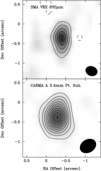
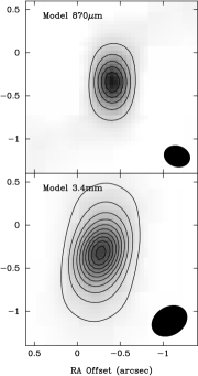
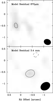
Figure 8: Model comparison: Images of L1527 (left) at 870 µm (top) and 3.4 mm (bottom) are shown, compared to models at the same wavelength (middle) and the residuals after subtracting the models from the data in the uv-plane (right). The models capture the general features seen in the high-resolution data. The most obvious discrepancy is the 3$\sigma$ residual on the southern side of the disk in the 3.4 mm image. The residual is also present in the SMA data, but at a lower level; this appears to be a disk asymmetry not captured by the model. The contours in all images start at 3$\sigma$ and increase in 3$\sigma$ intervals; $\sigma$ = 5.0 mJy beam^-1 (SMA), 0.24 mJy beam^-1 (CARMA 3.4 mm).

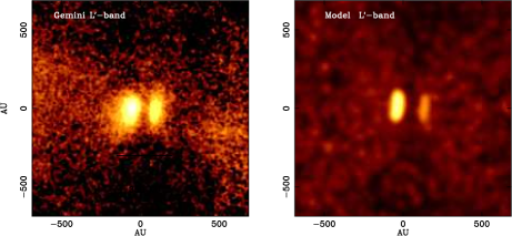
Figure 9: Observed L′ images of L1527 (left) compared to the best fitting model (right); the model is convolved with a Gaussian with FWHM of 0$\farcs$35 to match the seeing of the L′ observations. The scattered light from the model captures the brightest scattered light features of the disk well and reproduces the dark lane thickness.

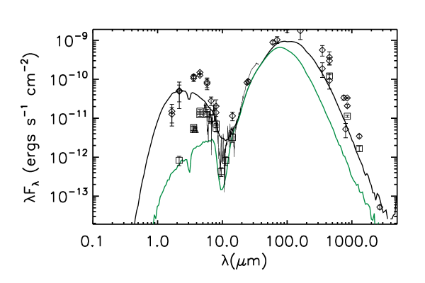
Figure 10: Model SED generated with the Whitney et al. (2003) radiative transfer code overlaid on the photometry data. The photometry and IRS spectrum are taken from Tobin et al. (2008, and references therein.). Photometry taken with apertures of 71$\farcs$4 (diamonds) and 7$\farcs$14 (boxes) (10000 AU and 1000 AU) are plotted. The triangle at 3.8 µm is the Gemini L′ flux within 1000 AU. The model SEDs are plotted for multiple model apertures of 10000 AU (black line), and 1000 AU (gray line). The model is somewhat deficient in flux at long wavelengths; however, this depends on both the level of external heating and the large-scale density profile and envelope structure. The IRS spectrum has a 3$\farcs$6 slit at wavelengths below 14 µm; at greater than 14 µm the slit size is 11″ wide, but aperture size does not matter in this range of wavelength since the emission is all from very small radii.

The visibilities of the best fitting models are overlaid on the data in Figure 7. In Figure 8, we show the model images at 870 µm  and 3.4 mm and the residuals when subtracted from the data. The model images reproduce the data quite well. Figure 9 shows the models compared to the observed L′ image; both models reproduce the locations of the brightest parts of scattered light well, but the more diffuse emission not reproduced by the models could be extended, upper layers of the disk or scattering in the outflow cavity. The SEDs of the best fitting model are shown in Figure 10; there is some deviation at wavelengths longer than 20 µm, but this may be due to disk vertical structure effects. We show the vertical density and temperatures profile at R = 100 AU for the model in Figure 11 as well as a hydrostatic equilibrium (HSEQ) calculation based on the equatorial density and vertical temperature distribution. This shows that the best fitting disk model has a vertical density profile about a factor of two larger vertical heights than HSEQ. A caveat here is that HSEQ density profile is calculated for the temperature profile of the best fit model, given that the density structure is different in HSEQ, the temperature profile will not be the same. Nonetheless, this serves as a simple demonstration of the disk model being more extended than HSEQ might allow. The parameters of the best fitting model is given in Table 5.

4.5 Comparison with Other Observations and Models

4.5.1 L1527

Previously, the highest resolution sub/millimeter data taken for L1527 were from the Plateau de Bure Interferometer (PdBI) at 1.3 mm (Maury et al., 2010). The CARMA and SMA data have modestly better resolution, but we were able to clearly resolve the disk and their observations did not. This was due to the elongation of the PdBI synthesized beam in the north-south direction, the same direction as the disk long axis. Jørgensen et al. (2009) used the SMA compact array data to infer the disk mass by assuming that the flux at 50 k$\lambda$ was primarily from the disk. The disk mass of L1527 was found to be 0.029 $M_{\sun}$ (assumed T = 30 K); when adjusted for our assumed value of $\kappa_{850\mu m}$, $M_{disk}$ = 0.015 $M_{\sun}$, larger but not inconsistent with our modeled value. There were also VLA 7mm observations of L1527 in A configuration that detected a small-scale disk with an apparent radius of 20 AU (Loinard et al., 2002), but with substantial spatial filtering. EVLA studies of L1527 are also underway with initial results from D configuration were presented by Melis et al. (2011).

4.5.2 Class 0 Sources

Other than Jørgensen et al. (2007, 2009) only a few studies have had the resolution to examine disks in Class 0 sources. Brown et al. (2000) used the JCMT-CSO interferometer to constrain disk radii in a few Class 0 sources to be $\sim$300 AU. Looney et al. (2000) surveyed a range of young stellar objects (Class 0 - II), finding evidence of a resolved disk around NGC 1333 IRAS 2A as well as some Class I sources. Chiang et al. (2012) observed L1157 with high-resolution using CARMA and do not find a resolved disk on 90 AU scales, while Lee et al. (2009) found indications of a disk in HH211 and a companion. Maury et al. (2010) published a high-resolution sample of 5 protostars observed with the PdBI (L1527 included), none of which showed strong signs of resolved disk emission. A large ($R$ = 300 AU), massive ($M_{disk}$ $\sim$ 1 $M_{\sun}$) disk was found around Serpens FIRS1 by Enoch et al. (2009); however, this system is likely intermediate mass with the revised/increased distance estimate toward Serpens. Finally, Harvey et al. (2003) examined the B335 system, inferring that there was a 0.004 $M_{\sun}$ disk from modeling the flattening visibility amplitudes, but they did not resolve the disk and only inferred a radius $<$ 100 AU. Thus, L1527 is currently in a class by itself when it comes to resolved disks in the Class 0 phase.

4.5.3 Class I & II sources

Several disks have been imaged in the infrared and submillimeter around Class I protostars with disk radii between 50 and 300 AU (e.g. Stark et al., 2006; Padgett et al., 1999). High-resolution dust continuum observations have been taken toward IRAS 04302+2247, finding $M_{disk}$ $\sim$ 0.07 $M_{\sun}$ and $R_{disk}$ = 300AU (Wolf et al., 2008). CB26 was also resolved in the near-infrared and millimeter by Launhardt et al. (2001), subsequent modeling by (Sauter et al., 2009) finds $M_{disk}$ $\sim$ 0.3 $M_{\sun}$ and $R_{disk}$ = 200 AU. The characteristic radii of Class II disks peaks at about 50 AU (Andrews et al., 2010), but extends to 100s of AU. These results indicate that the disk in L1527 already has a characteristic radius similar to Class I and II sources. The disk mass of 0.0075 $M_{\sun}$ for L1527 is quite comparable to what is found for Class I or II sources, but this is a poorly constrained quantity. The radial density profile of L1527 may also be steeper than the typical $\Sigma$ $\propto$ $R^{-1}$ found in Class II disks, but this quantity is not well-constrained since the disk is viewed edge-on. Exact parameters of the best fit model are compared to IRAS 04302+2247 and CB26 in Table 7.

The difference in observed scale-height between L1527 and Class I/II sources is the most striking. The models of Class I and II sources indicate typical values of $H_{100}$ to be about 10 - 15 AU (Sauter et al., 2009; Wolf et al., 2008; Andrews et al., 2010), while L1527 has $H_{100}$ = 48 AU. However, under the assumption of Gaussian vertical structure, L1527 is about a factor of two more vertically extended than HSEQ, as shown in Figure 11. However, in more evolved systems the scale heights may appear smaller due to dust settling. In the case of HL Tau, the disk was found to be 1.5$\times$ more vertically extended than HSEQ with H₁₀₀ = 19 AU (Kwon et al., 2011). The vertical height of the disk in L1527 appears to be substantially larger than in Class II disks.

5 Discussion

We have conducted radiative transfer modeling of the youngest protostellar system know to harbor a rotationally-supported disk in both sub/millimeter dust emission and near-infrared scattered light. The system was modeled with a disk surrounded by an infalling envelope with masses and radii typical of Class II disks (e.g. Andrews & Williams, 2007; Andrews et al., 2009, 2010), while the vertical height is substantially larger. The parameters of disks in these early stages represent the initial conditions of the Class I/II objects and indicate how likely a system might be to fragment gravitationally forming a binary system and/or giant planets. The principal difficultly in characterizing young disks thus far has been the surrounding envelope; at most size-scales, the emission is a combination of disk and envelope. Thus, in order to be certain that the disk is being detected, a system must be observed with sufficient resolution to resolve it and/or kinematic data must find rotationally supported motion. In the case of L1527, we have both resolved the disk in the dust continuum at multiple wavelengths and kinematic data show a rotation signature consistent with Keplerian rotation (Tobin et al., 2012).

5.1 Evolutionary State of L1527

Whether or not L1527 is a Class 0 or Class I protostar is an important distinction for this work as well as the implications for disk formation theory. It was previously discussed in Tobin et al. (2008) that L1527 would probably be classified as a Class I object if it were not viewed edge-on. This is because the submillimeter luminosity would no longer meet the criteria of being $\geq$ 0.5% of the bolometric luminosity (Andre et al., 1993), with a similar effect on the bolometric temperature. The classification of protostars as Class 0 based on bolometric temperature or submillimeter luminosity may be unreliable since all protostars seem to have outflow cavities and these diagnostics depend on inclination (Jørgensen et al., 2009). Moreover, the classification of a protostar as Class I is not exclusive of Class 0, since the Class I - III scheme is based on near to mid-infrared spectral indicies and Class 0 is based on submillimeter flux or bolometric temperature. Spitzer detects many well-known Class 0 protostars between 3.6 and 8µm with rising SED slopes out to 24/70 µm (Tobin et al., 2007; Jørgensen et al., 2006; Seale & Looney, 2008; Enoch et al., 2009; Tobin et al., 2010b) enabling them to be simultaneously classified as Class I and Class 0. Semantics aside, the main issue is whether or not L1527 is consistent with being a very young protostar or if it has evolved into a later phase.

Bonafide Class I sources in Taurus (e.g. IRAS 04302+2247) appear much more compact at IRAC wavelengths, and do not have the resolved outflow cavities extending out to $\sim$10000 AU as seen in L1527 (Hartmann et al., 2005). Furthermore, the envelopes of Class I protostars also have much more compact millimeter emission (i.e. L1489 IRS, Motte & André, 2001); L1527 has a large envelope resolved in the submillimeter (Chandler & Richer, 2000). On the other hand, L1527 differs from the more typical Class 0 objects that have more well-collimated outflows and do not have as intense scattered light nebulosities; Tobin et al. (2010b) shows examples of this. Independent of the photometric and image properties, Emprechtinger et al. (2009) showed that younger Class 0 sources typically have higher ratios of N₂D⁺ to N₂H⁺ than more evolved Class 0 or Class I sources. Toward the central protostar of L1527, there was not a detectable level of N₂D⁺, but there is N₂D⁺ at larger radii (Tobin et al., 2013).

The above discussion demonstrates that the observational Class of a particular system does not necessarily indicate the evolutionary state. Robitaille et al. (2006) attempted to alleviate this distinction by defining “stages”; however, these stages are based on model dependent quantities. Within this framework, however, L1527 is consistent with being a Stage 0/I protostar. Moreover, Andre et al. (1993) suggested that the observational classification of Class 0 would mean $M_{env}$ $>$ $M_{*}$ and the envelope mass of L1527 exceeds the protostellar mass by about factor of five (Shirley et al., 2000; Chandler & Richer, 2000; Tobin et al., 2010b). While L1527 does not conform to all the general properties of a Class 0 or Class I source, it is clearly in an early evolutionary state, but likely not among the youngest of Class 0 protostars.

5.2 Disk Structure

The radiative transfer modeling enabled us to derive likely values for structural parameters of the protostellar disk, within the limitations of our parametrized disk model. We find that a disk radius of 125 AU provides the best fit to the data. This is not terribly different from the 190 AU radius indicated in Paper I, but this value is likely more robust given the additional observational constraints. Moreover, this radius should not be thought of as a hard outer edge of the disk, and perhaps more as a transition point between and envelope-dominated density/kinematic structure and that of the disk. A more physical treatment of the disk-envelope interface may be necessary in future modeling to better understand the assembly of the proto-planetary disk.

The mass of the disk in L1527 is not large, only 0.0075 $M_{\sun}$, consistent with the optically thin calculation. However, this value should be regarded with extreme caution, give the uncertainties in $\beta$, assumed dust opacity law, and the dust to gas ratio (e.g. Ricci et al., 2010). While the dust opacity directly affects our measurement of the mass, it should not strongly affect the other properties of our model given that most of the emission is optically thin and we expect that $\kappa_{850\mu m}$ should be lower than our assumed value. We calculated that emission from our disk model, integrated along the line of sight, will become optically thick ($\tau$ = 1) at projected radial distances of 11.5 AU and 9 AU at 870 µm and 3.4 mm respectively; much smaller than our spatial resolution. The enclosed masses within 11.5 AU and 9 AU radii are 7.4 $\times$ 10^-4 $M_{\sun}$ and 6.1 $\times$ 10^-4 $M_{\sun}$, consistent with our simplistic mass measurements in Section 3.5 being smaller than the total mass of the model. Furthermore, there could be a dead zone at small radii that is optically thick, harboring a substantial amount of hidden mass and we would not know about it with the current observations. The brightness temperatures of the disk have a maximum value of T_B = 12 K at 870 µm, while the compact disk structure observed at 7 mm by (Loinard et al., 2002) has T_B = 50 K indicating that it may be optically thick at 7 mm.

A surprising result from our study is the large scale-height of the disk. The disk scale height $H$ is proportional to $R^{1.3}$, with $H_{100}$ = 48 AU. For comparison, the analytic solution for an irradiated disk is $H$ $\propto$ $R^{1.25}$ and $R^{1.125}$ for a steady, viscous accretion disk. Figure 10 shows the vertical density and temperature profiles of the disk in L1527. For comparison, the vertical hydrostatic equilibrium solution is also plotted assuming the same central density and dust temperature structure from the model. Using the dynamical mass measurement of 0.19 $M_{\sun}$, we find that the disk model is about a factor of two more extended than vertical HSEQ. Thus, even without the physics of the envelope infalling onto the disk, our model is able to reproduce the observations quite well; infall of the envelope onto the disk could make it more vertically extended than HSEQ.

The implied surface density profile is $\Sigma$ $\propto$ $R^{-1.2}$, inferred from $\rho$ $\propto$ $R^{-2.5}$ and $H$ $\propto$ $R^{1.3}$. While this parameter is not well-constrained, it is slightly steeper than the typical $\Sigma$ $\propto$ $R^{-1}$. This is expected for the more evolved systems because angular momentum transport from the mass accretion process will redistribute the mass from its initial configuration. We do caution that the best fit model has the minimum possible surface density distribution in the model grid. The implied surface density distribution by infall from a TSC envelope without mass redistribution is $\Sigma$ $\propto$ $R^{-1.5}$ (Hartmann, 2009); in agreement with one of our model cases. Our modeled surface density profile meets the criteria for gravitational instability of Toomre Q = 1 ($\Sigma$ $\propto$ $R^{-1.75}$), assuming T $\propto$ $R^{-3/4}$. However, if the disk mass is accurate, the protostar is more than order of magnitude more massive than the disk. $M_{disk}$ may be closer to $M_{*}$ in reality as the dust opacities may be over estimated and there could be optically thick dust on scales smaller than our beam. We caution that not too many conclusions can be drawn from the surface density profile because we are not directly sensitive to the surface density and must infer it from the radial and vertical structure.

5.3 Caveats

The best-fitting models of the disk-envelope system in L1527 are inherently non-unique. The models being employed represent the most idealized form of protostellar envelope and disk structures. Robust statistical measures can only be reliably used if the model is known to represent the observations a priori; therefore, meaningful confidence levels cannot be assigned to the model parameters. Given that we are modeling a protostellar system with known non-axisymmetries (Tobin et al., 2010b, 2011), the models cannot be expected to fully reproduce the observations. There are also degeneracies between certain parameters because of the edge-on orientation, as we will discuss later in this section. Moreover, some of the parameters fit may be abstractions of missing physics i.e. infall of the envelope onto the disk.

For instance, the radial density profile we find in the L1527 disk could be an artifact of our assumption of constant dust opacity at all radii. There could be preferentially smaller dust grains at large radii than at smaller radii, resulting from the influx of smaller grains from the infalling envelope and subsequent grain growth in the inner disk (Pérez et al., 2012). However, this scenario does not initially seem likely given that the spectral index of dust emission is constant at uv-distances $>$ 10 k$\lambda$ (Figure 6). One might expect that if the dust opacity were changing with radius in the disk and/or envelope, we would expect to see the spectral index change with uv-distance. But, 10 k$\lambda$ corresponds to spatial scales of $\sim$25″; Shirley et al. (2011) measures an integrated 3 mm flux density of 33 mJy toward L1527, consistent with our visibility amplitudes in Figure 4, suggesting that the disk is emitting most flux on these spatial scales and the envelope only becomes dominant at smaller spatial frequencies.

The degeneracies between parameters also adds uncertainty to our modeling. Some of the most significant degeneracies are: radial density profile to disk radius/mass/$\beta$, initial scale height to disk radius/flaring, and disk mass to $\beta$. However, we are able to mitigate but not retire these degeneracies with the SED fit to the IRS spectral range and the L′ image comparison. Higher resolution sub/millimeter data and fitting of the visibilities in two dimensions are both needed to better constrain disk parameters.

5.4 Millimeter-wave Dust Opacity

A particularly curious result is the low value of $\beta$, which we allowed to vary in our modeling. This could result from both systematic and astrophysical effects. An obvious culprit could be systematic errors in the absolute flux scale. Each dataset is calibrated as well as possible; the observations in different array configurations agree quite well in the regions of overlap in the uv-plane, even when different flux calibrators are used and when there were long time intervals between observations. Moreover, we did not find large discrepancies between our measured calibrator fluxes and those in the SMA and CARMA calibrator databases. Nonetheless, there is uncertainty in the planet models used for absolute flux calibration and there are differences between those used in MIRIAD for CARMA and those in MIR for the SMA. Variability of the source is another possibility, but the agreement of the measured flux over long time intervals seems to rule this out. Moreover, the SMA and CARMA observations at the highest resolution were taken a little over a month apart, mitigating the possibility of large flux variations.

Thus, the low value of $\beta$ seems to be real, confirming previous indications of a shallow $\beta$ (Melis et al., 2011; Scaife et al., 2012). In addition, previous single-dish observations of the envelope indicated $\beta$ $\sim$ 1 (Shirley et al., 2011). Moreover, observations of Class II sources in Taurus also show evidence for low values of $\beta$ (Andrews & Williams, 2005; Ricci et al., 2010) as well as Class 0 protostars (Kwon et al., 2009; Chiang et al., 2012); therefore, a shallow $\beta$ in the inner envelope and disk may be a realistic expectation.

The low value of $\beta$ can be explained by a population of large dust grains in the disk and inner envelope, as shown by opacity curves for large grains and different power-law size distributions (Hartmann, 2008; Ricci et al., 2010). The dust opacity models presented in Ricci et al. (2010) have $\kappa_{850\mu m}$ $\sim$ 2.5 cm² g^-1 (dust only opacity), with $\beta$ $\sim$0.25. Two models yield values of $\beta$ consistent with L1527, one with a power-law size distribution of $N(a)$ $\propto$ $a^{-2.5}$ and a maximum grain size of 1 cm, and another with $N(a)$ $\propto$ $a^{-3.0}$ and a maximum grain size of 10 cm. For comparison, we used $\kappa_{850\mu m}$ = 3.5 cm² g^-1 for the sub/millimeter modeling and $\kappa_{850\mu m}$ = 0.6 cm² g^-1 for the Monte Carlo model ($\beta$ $\sim$ 1.93); Ossenkopf & Henning (1994) gives $\kappa_{850\mu m}$ = 1.82 cm² g^-1 ($\beta$ $\sim$ 1.75). Thus, the Ricci et al. (2010) model seems attractive for the sub/millimeter regime and could adjust the disk mass upward by 1.6$\times$.

While, these opacity models for large dust grains are consistent with our observations, could such large dust grains have formed in the relatively short life of a Class 0 protostellar disk? Models of dust grain evolution considering the formation and growth of the disk, with infall from the envelope have been computed by Birnstiel et al. (2010). These models showed that grains can grow rapidly from micron-sizes to cm-sizes within $\sim$50 kyr, out to radii of $\sim$60 AU. Therefore, it seems possible that grain growth to cm-sizes could explain the shallow $\beta$. In addition, there is evidence that the dust grains in the envelopes are at least micron-sized (Pagani et al., 2010) and possibly larger (Shirley et al., 2011; Kwon et al., 2009; Chiang et al., 2012), so the disks may be seeded with larger grains to start with.

We note that any large dust grains must be concentrated in the disk, because larger grains throughout the envelope would broaden the 10 µm silicate absorption feature and observations show this feature to be quite sharp in Figure 10. This makes sense because grains will grow fastest where the densities are largest, i.e. the disk. Such large grains must also be settled to the disk midplane (Dullemond & Dominik, 2004; D’Alessio et al., 2006), because large dust grains throughout the disk would also cause the mid-infrared SED to from 10 µm to 70 µm to not fit the data (Tobin et al., 2010a). Furthermore, the larger the grains grow, the more rapidly they settle to the disk midplane; the settling timescale is shorter than the grain growth timescale (Dullemond & Dominik, 2004). Therefore, we suggest that a population of large dust grains, responsible for much of the emission at sub/millimeter wavelengths and shallow opacity spectral index, are settled in the disk midplane with a smaller scale height than the disk observed in scattered light. Nevertheless, it remains possible that much of the millimeter-wave emission is coming from an optically thick, dense disk midplane, similar to the model by (Gräfe et al., 2013) for IRAS 04302+2247. In this scenario, the upper layers of the disk, responsible for the L′ scattered light, are tracing a different size distribution of dust grains. However, recall that the millimeter-wave SED is consistent with $\beta$ $\sim$ 0 out to 7 mm, where we would certainly expect the emission to be optically thin.

5.5 Constraints on Disk Formation and Evolution

If L1527 reflects the state of disks toward the end of the Class 0 phase, then we can infer that disks must grow rapidly within the Class 0 phase, as it only lasts $\sim$ 0.5 Myr (Evans et al., 2009). Idealized magnetic collapse models predict that disks no greater than 10 AU would be observed in Class 0 systems, within 4 $\times$ 10⁴ yr of collapse Dapp & Basu (2010). A radius of 125 AU may be a bit larger than expected for such a young source (Dapp et al., 2011); however, we should expect to find a variety of disk radii in young protostellar systems, since star forming cores will have a variety of angular momenta (Goodman et al., 1993; Caselli et al., 2002; Chen et al., 2007; Tobin et al., 2011). Therefore, the models of Dapp et al. (2011) either need to start with more angular momentum or magnetic braking is not as effective at retarding the formation large disks as their models suggest. On the other hand, Vorobyov (2010) showed that disks similar in size to L1527 can form before the end of the Class 0 phase with only modest initial angular velocities, but this simulation ignores the effects of magnetic fields. Joos et al. (2012) then finds that large disks can form in ideal MHD simulations, but only if the initial magnetic field direction is misaligned with the outflow, a phenomenon that has been recently observed in a number of protostars, L1527 included (Hull et al., 2012).

Yorke & Bodenheimer (1999) also conducted simulations of disk formation in two dimensions, but in an edge-on axisymmetric geometry, also ignoring magnetic fields. Large disks also formed in these simulations; however, the disks (the low-mass Case H and J) have $H_{100}$ = 8 AU (extrapolated from given values at $R$ = 500, 1000 AU), substantially smaller than our models for L1527. The disks are highly flared ($H$ $\propto$ $R^{1.34}$), while the initial scale heights are quite small. Note that these values are from the end of the simulation, where the disk has grown to $R$ $>$ 1500 AU and the amount of mass in the sink cell is 0.6 $M_{\sun}$. The infall onto the disk does generate a shock, but this shock is $\sim$ 8 scale heights above the midplane, creating a $\sim$40 AU region of relatively constant density in the z direction. This shocked region could qualitatively explain the diffuse L′-band scattered light extended so high above the disk midplane, in addition to non-Gaussian vertical structure.

Overall, our results suggest that by the end of the Class 0 phase, it is possible for disks to have grown to a substantial fraction of their ultimate radius, as evidenced by Class I and II disks not being substantially larger than the disk in L1527. This is in agreement with hydrodynamic simulations and could be consistent with simulations that include magnetic fields, depending on initial conditions. The disk also must become substantially less flared and vertically extended between the Class 0 to Class I/II phases. This process likely involves both dust settling (D’Alessio et al., 2006) and contraction toward the midplane as the stellar mass grows to maintain HSEQ.

The observation of a shallow dust opacity spectral index in the disk of L1527, taken with the observations of $\beta$ $<$ 1 in other protostars (Kwon et al., 2009; Chiang et al., 2012) seems to indicate that grain growth may proceed rapidly during the protostellar phase. Thus, disks in the Class I/II phase may have already have large grains, perhaps enabling planetesimal growth at in the early in the star formation process.

5.6 Timescales for Disk and Protostellar Mass Growth

Given that, we have a constraint on the protostellar mass, the disk radius, and the large-scale velocity gradient from Tobin et al. (2011), we can compare these values to the Terebey et al. (1984) and Shu (1977) timescales for disk and protostellar growth. While these relationships are simplistic and ignore magnetic fields, they are illustrative of the timescales involved for disk assembly and mass accumulation. Following Hartmann (2009), $R_{C}$ grows as

$$R_{C}(t)=\frac{m_{\circ}^{3}}{16}c_{s}t^{3}\Omega_{\circ}^{2}$$ (5)

where $m_{\circ}$ = 0.975, $c_{s}$ = 0.2 km s^-1 and $\Omega_{\circ}$ = 2.2 km s^-1 pc^-1  (Tobin et al., 2011). The protostellar mass then grows as

$$M_{*}=\frac{m_{\circ}c_{s}^{3}t}{G}$$ (6)

where G is the gravitational constant. Application of these equations indicates that it would take 1.1 $\times$ 10⁵ yr for the protostar to accumulate 0.19 $M_{\sun}$ and 2.16 $\times$ 10⁵ yr to grow the disk to 125 AU, a factor of $\sim$2 difference. Thus, in the time it took to build the disk to 125 AU, the protostellar mass should be 0.4 $M_{\sun}$. This could mean that the additional mass is being built up in the disk, but it would have to be optically thick and on small spatial scales, below our resolution limit. Furthermore, the disk timescale hinges greatly on the assumed initial cloud rotation. Both Ohashi et al. (1997) & Tobin et al. (2011) show that the outer envelope velocity gradient is in the opposite direction of the disk rotation. If we instead adopt the inner envelope velocity gradient of 12.1 km s^-1 pc^-1 , the timescale form a 125 AU disk is reduced to 7 $\times$ 10⁴ yr, in closer agreement to the mass accretion timescale.

5.7 Future Prospects for Class 0 disks

In order to clearly detect the disk in L1527, we had to observe L1527 at the limit of angular resolution available to current millimeter interferometers (SMA, CARMA, and Cycle 0 ALMA). The disk in L1527 was not clearly resolved until it was observed with a spatial resolution roughly 5x finer than its modeled diameter. Therefore, we suggest that in order to detect disks embedded in dense envelopes, they must be over-resolved by a factor of about five compared to the expected diameter, in order to distinguish the disk from the envelope. Thus, with the current sub/millimeter interferometers, we should not expect to clearly resolve disks around Class 0 protostars in star forming regions more distant than Taurus or Perseus; even then only the largest Class 0 disks will be able to be resolved. When ALMA is fully online this landscape will change dramatically. Disks as small as 30 AU around the youngest protostars in Taurus should be resolved and 60 AU in Orion; the Jansky VLA also has this capability of observations at 7 mm. Therefore, the future prospects of resolving disks around Class 0 protostars may be much brighter than suggested by Maury et al. (2010) and Dapp et al. (2011). Moreover, the possibility of observe molecular line emission from the disks with ALMA should enable the masses of a large sample of Class 0 protostellar objects to be characterized.

6 Conclusions

We have presented analysis and radiative transfer modeling of high-resolution observations toward the protostar L1527 at $\lambda$ = 870 µm and 3.4 mm with the SMA and CARMA. We found that the protostellar system can be well-modeled with an extended disk, using the Monte Carlo radiative transfer codes of Whitney et al. (2003) and Brinch & Hogerheijde (2010).

1. We modeled the disk emission by fitting the one dimensional visibilities, sub/millimeter images, multi-wavelength SED, and L′ images. The best fitting model has a radius of 125 AU, mass of 0.0075 $M_{\sun}$, a radial density profiles proportional to $R^{-2.5}$, power-law flaring with $H$ $\propto$ $R^{1.3}$ (assuming Gaussian vertical structure), vertical scale heights at 100 AU of 48 AU, and a dust opacity spectral index of $\beta$ = 0.25. The most robust parameters are the disk radii and vertical height as these are well-constrained by the resolved image data in the sub/millimeter and L′ scattered light. The disk vertical structure is not drastically out of hydrostatic equilibrium, a factor of two larger, but this is subject to the assumptions of the Gaussian vertical density profile. The most degenerate parameters are the disk mass, radial density profile. The disk mass is dependent on the assumed dust opacity, the radial structure is not well enough resolved.

2. The millimeter spectral index from the integrated fluxes at 870 µm, 3.4 mm, and other work suggest a spectral slope in the millimeter of $S_{\lambda}$ $\propto$ $\lambda^{-2}$. Assuming optically thin and isothermal emission, this suggests that the dust opacity spectral index $\beta$ = 0. We then examined the spectral index from 870 µm to 3.4 mm as a function of uv-distance, finding that at all spatial scales $\beta$ is consistent with zero. The modeled dust opacity spectral index of 0.25 is consistent with the shallow spectral index. This is the shallowest known spectral index for a Class 0 protostar and bears similarity to what has been observed for more evolved Class II sources. This result suggests that the dust opacities may have a shallow power-law size distribution and maximum grain sizes of 1 - 10 cm. Models of grain growth show that rapid growth to cm sizes is possible within the timescale of the Class 0 phase; thus, Class I/II disks may already start with large dust grains.

3. L1527 appears most consistent with a late Class 0 source, but shares some characteristics of both Class I and Class 0 protostars. Comparing the disk properties to Class I/II sources, we find L1527 to have a smaller radius and less flared, possibly indicating an evolutionary trend of sustained disk growth and settling into the Class I phase.

Facilities: Gemini:Gillett (NIRI), VLA, CARMA, SMA

The authors wish to thank the anonymous referee for comments which improved the manuscript. J. T. acknowledges support provided by NASA through Hubble Fellowship grant #HST-HF-51300.01-A awarded by the Space Telescope Science Institute, which is operated by the Association of Universities for Research in Astronomy, Inc., for NASA, under contract NAS 5-26555. L. H. and J. T. acknowledge partial support from the University of Michigan. H.-F. C. acknowledges support from the National Aeronautics and Space Administration through the NASA Astrobiology Institute under Cooperative Agreement No. NNA09DA77A issued through the Office of Space Science. L.W.L. and H.-F. C. acknowledge support from the Laboratory for Astronomical Imaging at the University of Illinois and the NSF under grant AST-07-09206. P. D. acknowledges a grant from PAPIIT-UNAM. L. L. acknowledges the support of DGAPA, UNAM, CONACyT (México), and the Alexander von Humboldt Stiftung for financial support. Support for CARMA construction was derived from the states of Illinois, California, and Maryland, the James S. McDonnell Foundation, the Gordon and Betty Moore Foundation, the Kenneth T. and Eileen L. Norris Foundation, the University of Chicago, the Associates of the California Institute of Technology, and the National Science Foundation. Ongoing CARMA development and operations are supported by the National Science Foundation under a cooperative agreement, and by the CARMA partner universities. The Submillimeter Array is a joint project between the Smithsonian Astrophysical Observatory and the Academia Sinica Institute of Astronomy and Astrophysics and is funded by the Smithsonian Institution and the Academia Sinica. The National Radio Astronomy Observatory is a facility of the National Science Foundation operated under cooperative agreement by Associated Universities, Inc.

Figure 4: Plots of visibility amplitude versus projected baseline for the SMA 870 µm, CARMA 3.4 mm, CARMA 3.4 mm point-source subtracted. The different symbols represent different binning of the visibility data in the uv-plane, in 10 k$\lambda$ bins (plus-signs) and 50 k$\lambda$ bins (diamonds). The relative shapes of the visibility curves in the CARMA and SMA data are similar; the CARMA 3.4 mm visibilities without the point-source subtracted flatten-out longward of 300k$\lambda$ at $\sim$1.8 mJy. The fact that the SMA data show no similar flattening further motivates the subtraction of the point-source as contaminating free-free emission. The uncertainties are only statistical, not including the absolute calibration uncertainty. The dashed line which is near zero at short uv-distances represents the expected visibility amplitude from a blank field.

Figure 5: SED of L1527 from 870 µm to 6.5 cm; points longward of 3.4 mm are from Melis et al. (2011). The 870 µm and 3.4 mm points are measured from the naturally weighted images in the very extended and CARMA A configurations respectively. The dashed line is the fit to the free-free jet emission in the centimeter (Melis et al., 2011) with a spectral index of 0.33; the solid line is a power law with a spectral index of 2 (Rayleigh-Jeans). The square points are the measured photometry without correction for free-free emission and the diamonds have the free-free emission subtracted. The error bars are only statistical uncertainties, not including the $\sim$10% error in flux calibration.

Figure 6: Spectral index of emission between 870 µm and 3.4 mm emission. Assuming optically thin emission, the spectral index is equal to 2 + $\beta$ in the Rayleigh-Jeans limit. The L1527 data are consistent with $\beta$ $\sim$ 0 across all uv distances. The errorbars include both statistical uncertainty and 20% flux calibration uncertainty at each wavelength.

Figure 7: Visibilities of L1527 at 870 µm (left) and 3.4 mm (right) are plotted as the points (same as Figure 4. The lines represent the best overall model reproducing the visibility data.

Figure 11: Plot of disk density (left) and dust temperature (right) at $R$ = 100 AU as a function of distance above the midplane (Z) for the best fitting model. A hydrostatic equilibrium (HSEQ) solution is also plotted for the same central density and the temperatures shown in the right panel (dot-dashed line). The best fitting disk model disk for L1527 is more extended than HSEQ given the input temperature profile. The midplane temperature is quite warm compared to Class II disks, the 30 K central temperature implies that CO will not be frozen out and molecules should be present in the gas.

Table 1: CARMA 3.4 mm Observations

Source	RA	Dec	Config.	Date	Calibrators
	(J2000)	(J2000)		(UT)	(Gain, Flux)
L1527	04:39:53.9	+26:03:09.6	E-array	02, 05, 06 Oct 2008	3C111, 3C84
L1527	…	…	D-array	28, 30 Jul 2009	3C111, Mars
L1527	…	…	D-array	31 Aug 2008	3C111, Uranus
L1527	…	…	C-array	28 May 2009	3C111, 3C84
L1527	…	…	C-array	11 Oct 2009	3C111, Uranus
L1527	…	…	B-array	02 Jan 2010	3C111, Uranus
L1527	…	…	B-array	06 Jan 2010	3C111, None
L1527	…	…	A-array	02 Dec 2010	3C111, Neptune

Note. —

Table 2: SMA 870 µm Observations

Source	RA	Dec	Config.	Date	Calibrators
	(J2000)	(J2000)		(UT)	(Gain, Flux)
L1527	04:39:53.9	+26:03:09.6	Compact	17 Dec 2004	3C111, Uranus
L1527	…	…	Very Extended	05/06 Jan 2011	3C111, Callisto

Table 3: L1527 Millimeter Fluxes

Wavelength	Configuration(s)	Integrated Flux	Peak Flux	Gaussian Size	Gaussian PA	Deconvolved Size	Deconvolved PA	Robust	Taper	Beam
(mm)		(mJy)	(mJy)	(″)	(°)	(″)	(°)		(″)	(″)
3.4	A	16.9$\pm$1.4	7.1$\pm$0.3	0.6 $\times$ 0.50	-1.8	0.55 $\times$ 0.246	6.6	2	…	0.43 $\times$ 0.33
0.87	VEX	213.6$\pm$8.1	80.8$\pm$5.7	0.55 $\times$ 0.24	-1.5	0.54 $\times$ 0.14	-3.6	2	…	0.30 $\times$ 0.24
3.4	ABCDE	22.5$\pm$1.8	20.5$\pm$0.6	…	…	…	…	2	2.0	2.2 $\times$ 2.0
0.87	VEX + COMP	235.5$\pm$5.8	160.6$\pm$4.8	…	…	…	…	2	…	0.62 $\times$ 0.49

Note. — Note that the uncertainties are only statistical.

Table 4: Model Grid Parameters

Parameter	Description	Values
R∗(R☉)	Stellar radius	2.09
T∗(K)	Stellar temperature	4000
L∗(L☉)	System luminosity	2.75
M∗(M☉)	Stellar mass	0.5
Mdisk(M☉)	Disk mass	0.005, 0.0075, 0.01, 0.025, 0.05, 0.075, 0.1
Rdisk,max/Rc(AU)	Disk Radius	50.0, 100.0, 125.0, 150.0, 175.0, 200.0, 250.0, 300.0
H0 (R∗)	Disk scale height at R∗	0.02, 0.025, 0.03, 0.035
$p$	Disk radial density exponent	2.5, 3.0, 3.5, 4.0
$\gamma$	Disk scale height exponent	1.22, 1.25, 1.27, 1.3
$\dot{M}_{disk}$(M☉ $yr^{-1}$)	Disk accretion rate	3.0 $\times 10^{-7}$
Rtrunc(R∗)	Magnetosphere co-rotation radius	3.0
Fspot	Fractional area of accretion hotspot	0.01
Rdisk,min(R∗)	Disk inner radius	14.25
Renv,min(R∗)	Envelope inner radius	42.75
Renv,max(AU)	Envelope outer radius	15000
$\dot{M}_{env}$(M☉ $yr^{-1}$)	Envelope mass infall rate	1.0 $\times 10^{-5}$
bout	Outer cavity shape exponent	1.5
$\theta_{open,out}$(∘)	Outer cavity opening angle	20
$\theta_{inc}$(∘)	Inclination angle	85
$\rho_{c}$(g cm-3)	Cavity density	0
$\kappa_{850\mu m}$(cm2 g-1)	Dust opacity at 850µm	3.5
$\beta_{dust}$	Dust Spectral Index Disk/Envelope	0.0 0.25 0.5 0.75

Table 5: Model parameters

Parameter	Description	Paper I Model	Best Fit Model	Parameter Use
R∗(R☉)	Stellar radius	2.09	2.09	fixed
T∗(K)	Stellar temperature	4000	4000	fixed
L∗(L☉)	System luminosity	2.75	2.75	fixed
M∗(M☉)	Stellar mass	0.5	0.19	fixed
Mdisk(M☉)	Disk mass	0.005	0.0075	varied
h(100AU)	Disk scale height at 100AU	36.3	48.0	varied
H0	Disk scale height at R∗	0.03	0.03	varied
$p$	Disk radial density exponent	3.0	2.5	varied
$\gamma$	Disk scale height exponent	1.27	1.3	varied
$\dot{M}_{disk}$(M☉ $yr^{-1}$)	Disk accretion rate	3.0 $\times 10^{-7}$	1.5 $\times 10^{-6}$	fixed
Rtrunc(R∗)	Magnetosphere co-rotation radius	3.0	3.0	fixed
Fspot	Fractional area of accretion hotspot	0.01	0.01	fixed
Rdisk,min(R∗)	Disk inner radius	14.25	14.25	fixed
Rdisk,max/Rc(AU)	Disk outer radius	190	125	varied
Renv,min(R∗)	Envelope inner radius	42.75	42.75	fixed
Renv,max(AU)	Envelope outer radius	15000	15000	fixed
$\dot{M}_{env}$(M☉ $yr^{-1}$)	Envelope mass infall rate	0.8 $\times 10^{-5}$	4.5 $\times 10^{-6}$	fixed
$\rho_{1AU}$(g cm-3)	Envelope density at 1AU	5.8 $\times 10^{-14}$	7.25 $\times 10^{-14}$	varied
bout	Outer cavity shape exponent	1.5	1.5	fixed
$\theta_{open,out}$(∘)	Outer cavity opening angle	20	20	fixed
$\theta_{inc}$(∘)	Inclination angle	85	85	fixed
$\rho_{c}$(g cm-3)	Cavity density	0	0	fixed
$\beta_{dust,mm}$	Millimeter Dust Spectral Index	…	0.25	varied

Table 6: Parameter Ranges From Fitting

Weighted Data	Number of Models	Rdisk	Mdisk	$\alpha_{disk}$	$H(r)$	$H_{init}$	$\beta$
		(AU)	($M_{\sun}$)			($R_{*}$)
Uniform Weighting	032	125${}^{200}_{100}$	0.0075${}^{0.010}_{0.005}$	2.5${}^{3.0}_{2.5}$	1.30${}^{1.30}_{1.25}$	0.030${}^{0.035}_{0.020}$	0.25${}^{0.25}_{0.00}$
SED, IRS, Visibilities, and Sub/mm images	052	100${}^{300}_{100}$	0.0100${}^{0.100}_{0.007}$	2.5${}^{3.5}_{2.5}$	1.25${}^{1.30}_{1.22}$	0.025${}^{0.035}_{0.020}$	0.25${}^{0.50}_{0.25}$
Visibilities and Sub/mm images	056	100${}^{300}_{100}$	0.0075${}^{0.100}_{0.005}$	2.5${}^{3.5}_{2.5}$	1.27${}^{1.30}_{1.22}$	0.035${}^{0.035}_{0.020}$	0.25${}^{0.50}_{0.00}$
Visibilities	120	100${}^{300}_{100}$	0.0075${}^{0.100}_{0.005}$	2.5${}^{3.5}_{2.5}$	1.27${}^{1.30}_{1.22}$	0.030${}^{0.035}_{0.020}$	0.25${}^{0.75}_{0.25}$
Sub/mm images	024	100${}^{175}_{100}$	0.0075${}^{0.025}_{0.005}$	2.5${}^{3.0}_{2.5}$	1.27${}^{1.30}_{1.22}$	0.035${}^{0.035}_{0.020}$	0.25${}^{0.50}_{0.00}$
SED and IRS spectrum	209	200${}^{300}_{100}$	0.0100${}^{0.075}_{0.005}$	3.0${}^{3.5}_{2.5}$	1.27${}^{1.30}_{1.22}$	0.025${}^{0.035}_{0.020}$	0.00${}^{0.75}_{0.00}$
SED, IRS spectrum, and L′ image	037	150${}^{175}_{125}$	0.0075${}^{0.010}_{0.005}$	3.0${}^{3.0}_{2.5}$	1.27${}^{1.30}_{1.25}$	0.030${}^{0.035}_{0.025}$	0.00${}^{0.50}_{0.00}$
L′ image	016	125${}^{300}_{125}$	0.0050${}^{0.100}_{0.005}$	3.0${}^{4.0}_{2.5}$	1.30${}^{1.30}_{1.27}$	0.035${}^{0.035}_{0.025}$	0.00${}^{0.25}_{0.00}$
L′ and Sub/mm images	045	150${}^{200}_{100}$	0.0075${}^{0.010}_{0.005}$	2.5${}^{3.0}_{2.5}$	1.27${}^{1.30}_{1.25}$	0.030${}^{0.035}_{0.020}$	0.00${}^{0.25}_{0.00}$

Note. — We show the parameters of the models with $\chi^{2}$ - $\chi_{best}^{2}$ $<$ 3 (Robitaille et al., 2007); except for the L′ image and L′ + sub/mm images, where we chose $\chi^{2}$ - $\chi_{best}^{2}$ $<$ 8 in order to get a larger sampling of models. To give certain datasets more weight, we multiplied the respective $\chi^{2}$ by 10 The best fitting value is given in each column with the upper and lower ranges as superscripts and subscripts. Looking at the fits in this way better shows which sets of data constrain which values. It is clear that the data which do not take into account the spatial structure of the source (visibilities, SED, and IRS spectrum) do not provide adequate constraints on the models. The images do provide the best constraints on the source properties, but the additional constraints from the visibilities and SED/IRS are able to rule out some additional models.

Table 7: Model Parameter Comparisons

Parameter	Description	L1527	CB26	IRAS 04302+2247
Mdisk(M☉)	Disk mass	0.0075	0.3	0.07
h(100AU)	Disk scale height at 100 AU	48	10	15
$p$	Disk radial density exponent	2.5	2.2	2.37
$\gamma$	Disk scale height exponent	1.3	1.27	1.29
Rdisk,max(AU)	Disk outer radius	125	200	300
$\kappa_{dust,850\mu m}$ (cm2 g-1)	Millimeter Dust Opacity	3.5	2.5	2.5
$\beta_{dust,mm}$	Millimeter Dust Spectral Index	0.25	…	…

References

- Allen et al. (2003) Allen, A., Li, Z., & Shu, F. H. 2003, ApJ, 599, 363
- Andre et al. (1993) Andre, P., Ward-Thompson, D., & Barsony, M. 1993, ApJ, 406, 122
- Andrews & Williams (2005) Andrews, S. M., & Williams, J. P. 2005, ApJ, 631, 1134
- Andrews & Williams (2007) —. 2007, ApJ, 659, 705
- Andrews et al. (2009) Andrews, S. M., Wilner, D. J., Hughes, A. M., Qi, C., & Dullemond, C. P. 2009, ApJ, 700, 1502
- Andrews et al. (2010) —. 2010, ApJ, 723, 1241
- Birnstiel et al. (2010) Birnstiel, T., Dullemond, C. P., & Brauer, F. 2010, A&A, 513, A79
- Brinch & Hogerheijde (2010) Brinch, C., & Hogerheijde, M. R. 2010, A&A, 523, A25
- Brown et al. (2000) Brown, D. W., Chandler, C. J., Carlstrom, J. E., Hills, R. E., Lay, O. P., Matthews, B. C., Richer, J. S., & Wilson, C. D. 2000, MNRAS, 319, 154
- Calvet et al. (2005) Calvet, N., D’Alessio, P., Watson, D. M., Franco-Hernández, R., Furlan, E., Green, J., Sutter, P. M., Forrest, W. J., Hartmann, L., Uchida, K. I., Keller, L. D., Sargent, B., Najita, J., Herter, T. L., Barry, D. J., & Hall, P. 2005, ApJ, 630, L185
- Caselli et al. (2002) Caselli, P., Benson, P. J., Myers, P. C., & Tafalla, M. 2002, ApJ, 572, 238
- Cassen & Moosman (1981) Cassen, P., & Moosman, A. 1981, Icarus, 48, 353
- Chandler & Richer (2000) Chandler, C. J., & Richer, J. S. 2000, ApJ, 530, 851
- Chen et al. (2007) Chen, X., Launhardt, R., & Henning, T. 2007, ApJ, 669, 1058
- Chiang et al. (2008) Chiang, H., Looney, L. W., Tassis, K., Mundy, L. G., & Mouschovias, T. C. 2008, ApJ, 680, 474
- Chiang et al. (2012) Chiang, H., Looney, L. W., & Tobin, J. J. 2012, ApJ, 709, 470
- D’Alessio et al. (2001) D’Alessio, P., Calvet, N., & Hartmann, L. 2001, ApJ, 553, 321
- D’Alessio et al. (2006) D’Alessio, P., Calvet, N., Hartmann, L., Franco-Hernández, R., & Servín, H. 2006, ApJ, 638, 314
- Dapp & Basu (2010) Dapp, W. B., & Basu, S. 2010, A&A, 521, L56+
- Dapp et al. (2011) Dapp, W. B., Basu, S., & Kunz, M. W. 2011, ArXiv e-prints
- Dullemond & Dominik (2004) Dullemond, C. P., & Dominik, C. 2004, A&A, 421, 1075
- Dutrey et al. (1996) Dutrey, A., Guilloteau, S., Duvert, G., Prato, L., Simon, M., Schuster, K., & Menard, F. 1996, A&A, 309, 493
- Eisner (2012) Eisner, J. A. 2012, ApJ, 755, 23
- Emprechtinger et al. (2009) Emprechtinger, M., Caselli, P., Volgenau, N. H., Stutzki, J., & Wiedner, M. C. 2009, A&A, 493, 89
- Enoch et al. (2009) Enoch, M. L., Evans, N. J., Sargent, A. I., & Glenn, J. 2009, ApJ, 692, 973
- Espaillat et al. (2007) Espaillat, C., Calvet, N., D’Alessio, P., Hernández, J., Qi, C., Hartmann, L., Furlan, E., & Watson, D. M. 2007, ApJ, 670, L135
- Espaillat et al. (2008) Espaillat, C., Calvet, N., Luhman, K. L., Muzerolle, J., & D’Alessio, P. 2008, ApJ, 682, L125
- Evans et al. (2009) Evans, N. J., Dunham, M. M., Jørgensen, J. K., Enoch, M. L., Merín, B., van Dishoeck, E. F., Alcalá, J. M., Myers, P. C., Stapelfeldt, K. R., Huard, T. L., Allen, L. E., Harvey, P. M., van Kempen, T., Blake, G. A., Koerner, D. W., Mundy, L. G., Padgett, D. L., & Sargent, A. I. 2009, ApJS, 181, 321
- Galli et al. (2006) Galli, D., Lizano, S., Shu, F. H., & Allen, A. 2006, ApJ, 647, 374
- Goodman et al. (1993) Goodman, A. A., Benson, P. J., Fuller, G. A., & Myers, P. C. 1993, ApJ, 406, 528
- Gräfe et al. (2013) Gräfe, C., Wolf, S., Guilloteau, S., Dutrey, A., Stapelfeldt, K., Pontoppidan, K., & Sauter, J. 2013, ArXiv e-prints
- Hartmann (2008) Hartmann, L. 2008, Physica Scripta Volume T, 130, 014012
- Hartmann (2009) —. 2009, Accretion Processes in Star Formation: Second Edition, ed. Hartmann, L. (Cambridge University Press)
- Hartmann et al. (2005) Hartmann, L., Megeath, S. T., Allen, L., Luhman, K., Calvet, N., D’Alessio, P., Franco-Hernandez, R., & Fazio, G. 2005, ApJ, 629, 881
- Harvey et al. (2003) Harvey, D. W. A., Wilner, D. J., Myers, P. C., & Tafalla, M. 2003, ApJ, 596, 383
- Hennebelle & Fromang (2008) Hennebelle, P., & Fromang, S. 2008, A&A, 477, 9
- Ho et al. (2004) Ho, P. T. P., Moran, J. M., & Lo, K. Y. 2004, ApJ, 616, L1
- Hughes et al. (2009) Hughes, A. M., Andrews, S. M., Espaillat, C., Wilner, D. J., Calvet, N., D’Alessio, P., Qi, C., Williams, J. P., & Hogerheijde, M. R. 2009, ApJ, 698, 131
- Hull et al. (2012) Hull, C. L. H., Plambeck, R. L., Bolatto, A. D., Bower, G. C., Carpenter, J. M., Crutcher, R. M., Fiege, J. D., Franzmann, E., Hakobian, N. S., Heiles, C., Houde, M., Hughes, A. M., Jameson, K., Kwon, W., Lamb, J. W., Looney, L. W., Matthews, B. C., Mundy, L., Pillai, T., Pound, M. W., Stephens, I. W., Tobin, J. J., Vaillancourt, J. E., Volgenau, N. H., & Wright, M. C. H. 2012, ArXiv e-prints
- Isella et al. (2009) Isella, A., Carpenter, J. M., & Sargent, A. I. 2009, ApJ, 701, 260
- Joos et al. (2012) Joos, M., Hennebelle, P., & Ciardi, A. 2012, A&A, 543, A128
- Jørgensen et al. (2007) Jørgensen, J. K., Bourke, T. L., Myers, P. C., Di Francesco, J., van Dishoeck, E. F., Lee, C., Ohashi, N., Schöier, F. L., Takakuwa, S., Wilner, D. J., & Zhang, Q. 2007, ApJ, 659, 479
- Jørgensen et al. (2006) Jørgensen, J. K., Harvey, P. M., Evans, II, N. J., Huard, T. L., Allen, L. E., Porras, A., Blake, G. A., Bourke, T. L., Chapman, N., Cieza, L., Koerner, D. W., Lai, S., Mundy, L. G., Myers, P. C., Padgett, D. L., Rebull, L., Sargent, A. I., Spiesman, W., Stapelfeldt, K. R., van Dishoeck, E. F., Wahhaj, Z., & Young, K. E. 2006, ApJ, 645, 1246
- Jørgensen et al. (2009) Jørgensen, J. K., van Dishoeck, E. F., Visser, R., Bourke, T. L., Wilner, D. J., Lommen, D., Hogerheijde, M. R., & Myers, P. C. 2009, A&A, 507, 861
- Kitamura et al. (2002) Kitamura, Y., Momose, M., Yokogawa, S., Kawabe, R., Tamura, M., & Ida, S. 2002, ApJ, 581, 357
- Kwon et al. (2011) Kwon, W., Looney, L. W., & Mundy, L. G. 2011, ApJ, 741, 3
- Kwon et al. (2009) Kwon, W., Looney, L. W., Mundy, L. G., Chiang, H.-F., & Kemball, A. J. 2009, ApJ, 696, 841
- Lada (1987) Lada, C. J. 1987, in IAU Symp. 115: Star Forming Regions, ed. M. Peimbert & J. Jugaku, 1–17
- Launhardt et al. (2001) Launhardt, R., Sargent, A., & Zinnecker, H. 2001, in Astronomical Society of the Pacific Conference Series, Vol. 235, Science with the Atacama Large Millimeter Array, ed. A. Wootten, 134–+
- Lee et al. (2009) Lee, C., Hirano, N., Palau, A., Ho, P. T. P., Bourke, T. L., Zhang, Q., & Shang, H. 2009, ApJ, 699, 1584
- Li et al. (2011) Li, Z.-Y., Krasnopolsky, R., & Shang, H. 2011, ApJ, 738, 180
- Loinard et al. (2002) Loinard, L., Rodríguez, L. F., D’Alessio, P., Wilner, D. J., & Ho, P. T. P. 2002, ApJ, 581, L109
- Looney et al. (2000) Looney, L. W., Mundy, L. G., & Welch, W. J. 2000, ApJ, 529, 477
- Looney et al. (2003) —. 2003, ApJ, 592, 255
- Machida et al. (2010) Machida, M. N., Inutsuka, S.-i., & Matsumoto, T. 2010, ApJ, 724, 1006
- Maury et al. (2010) Maury, A. J., André, P., Hennebelle, P., Motte, F., Stamatellos, D., Bate, M., Belloche, A., Duchêne, G., & Whitworth, A. 2010, A&A, 512, A40+
- Melis et al. (2011) Melis, C., Duchêne, G., Chomiuk, L., Palmer, P., Perrin, M. D., Maddison, S. T., Ménard, F., Stapelfeldt, K., Pinte, C., & Duvert, G. 2011, ApJ, 739, L7+
- Mellon & Li (2008) Mellon, R. R., & Li, Z.-Y. 2008, ApJ, 681, 1356
- Motte & André (2001) Motte, F., & André, P. 2001, A&A, 365, 440
- Ohashi et al. (1997) Ohashi, N., Hayashi, M., Ho, P. T. P., & Momose, M. 1997, ApJ, 475, 211
- Ossenkopf & Henning (1994) Ossenkopf, V., & Henning, T. 1994, A&A, 291, 943
- Padgett et al. (1999) Padgett, D. L., Brandner, W., Stapelfeldt, K. R., Strom, S. E., Terebey, S., & Koerner, D. 1999, AJ, 117, 1490
- Pagani et al. (2010) Pagani, L., Steinacker, J., Bacmann, A., Stutz, A., & Henning, T. 2010, Science, 329, 1622
- Pérez et al. (2012) Pérez, L. M., Carpenter, J. M., Chandler, C. J., Isella, A., Andrews, S. M., Ricci, L., Calvet, N., Corder, S. A., Deller, A. T., Dullemond, C. P., Greaves, J. S., Harris, R. J., Henning, T., Kwon, W., Lazio, J., Linz, H., Mundy, L. G., Sargent, A. I., Storm, S., Testi, L., & Wilner, D. J. 2012, ArXiv e-prints
- Pérez et al. (2010) Pérez, L. M., Lamb, J. W., Woody, D. P., Carpenter, J. M., Zauderer, B. A., Isella, A., Bock, D. C., Bolatto, A. D., Carlstrom, J., Culverhouse, T. L., Joy, M., Kwon, W., Leitch, E. M., Marrone, D. P., Muchovej, S. J., Plambeck, R. L., Scott, S. L., Teuben, P. J., & Wright, M. C. H. 2010, ApJ, 724, 493
- Piétu et al. (2006) Piétu, V., Dutrey, A., Guilloteau, S., Chapillon, E., & Pety, J. 2006, A&A, 460, L43
- Reipurth et al. (2002) Reipurth, B., Rodríguez, L. F., Anglada, G., & Bally, J. 2002, AJ, 124, 1045
- Ricci et al. (2010) Ricci, L., Testi, L., Natta, A., Neri, R., Cabrit, S., & Herczeg, G. J. 2010, A&A, 512, A15
- Robitaille et al. (2007) Robitaille, T. P., Whitney, B. A., Indebetouw, R., & Wood, K. 2007, ApJS, 169, 328
- Robitaille et al. (2006) Robitaille, T. P., Whitney, B. A., Indebetouw, R., Wood, K., & Denzmore, P. 2006, ApJS, 167, 256
- Sault et al. (1995) Sault, R. J., Teuben, P. J., & Wright, M. C. H. 1995, in Astronomical Society of the Pacific Conference Series, Vol. 77, Astronomical Data Analysis Software and Systems IV, ed. R. A. Shaw, H. E. Payne, & J. J. E. Hayes, 433–+
- Sauter et al. (2009) Sauter, J., Wolf, S., Launhardt, R., Padgett, D. L., Stapelfeldt, K. R., Pinte, C., Duchêne, G., Ménard, F., McCabe, C.-E., Pontoppidan, K., Dunham, M., Bourke, T. L., & Chen, J.-H. 2009, A&A, 505, 1167
- Scaife et al. (2012) Scaife, A. M. M., Buckle, J. V., Ainsworth, R. E., Davies, M., Franzen, T. M. O., Grainge, K. J. B., Hobson, M. P., Hurley-Walker, N., Lasenby, A. N., Olamaie, M., Perrott, Y. C., Pooley, G. G., Ray, T. P., Richer, J. S., Rodríguez-Gonzálvez, C., Saunders, R. D. E., Schammel, M. P., Scott, P. F., Shimwell, T., Titterington, D., & Waldram, E. 2012, MNRAS, 420, 3334
- Seale & Looney (2008) Seale, J. P., & Looney, L. W. 2008, ApJ, 675, 427
- Seifried et al. (2012) Seifried, D., Banerjee, R., Pudritz, R. E., & Klessen, R. S. 2012, MNRAS, 423, L40
- Shirley et al. (2000) Shirley, Y. L., Evans, II, N. J., Rawlings, J. M. C., & Gregersen, E. M. 2000, ApJS, 131, 249
- Shirley et al. (2011) Shirley, Y. L., Mason, B. S., Mangum, J. G., Bolin, D. E., Devlin, M. J., Dicker, S. R., & Korngut, P. M. 2011, AJ, 141, 39
- Shu (1977) Shu, F. H. 1977, ApJ, 214, 488
- Stark et al. (2006) Stark, D. P., Whitney, B. A., Stassun, K., & Wood, K. 2006, ApJ, 649, 900
- Takakuwa et al. (2012) Takakuwa, S., Saito, M., Lim, J., Saigo, K., Sridharan, T. K., & Patel, N. A. 2012, ApJ, 754, 52
- Terebey et al. (1984) Terebey, S., Shu, F. H., & Cassen, P. 1984, ApJ, 286, 529
- Tobin et al. (2013) Tobin, J. J., Bergin, E. A., Hartmann, L., Lee, J.-E., Maret, S., Myers, P. C., Looney, L. W., Chiang, H.-F., & Friesen, R. 2013, ApJ, 765, 18
- Tobin et al. (2008) Tobin, J. J., Hartmann, L., Calvet, N., & D’Alessio, P. 2008, ApJ, 679, 1364
- Tobin et al. (2011) Tobin, J. J., Hartmann, L., Chiang, H.-F., Looney, L. W., Bergin, E. A., Chandler, C. J., Masqué, J. M., Maret, S., & Heitsch, F. 2011, ApJ, 740, 45
- Tobin et al. (2012) Tobin, J. J., Hartmann, L., Chiang, H.-F., Wilner, D. J., Looney, L. W., Loinard, L., Calvet, N., & D’Alessio, P. 2012, Nature, 492, 83
- Tobin et al. (2010a) Tobin, J. J., Hartmann, L., & Loinard, L. 2010a, ApJ, 722, L12
- Tobin et al. (2010b) Tobin, J. J., Hartmann, L., Looney, L. W., & Chiang, H. 2010b, ApJ, 712, 1010
- Tobin et al. (2007) Tobin, J. J., Looney, L. W., Mundy, L. G., Kwon, W., & Hamidouche, M. 2007, ApJ, 659, 1404
- Ulrich (1976) Ulrich, R. K. 1976, ApJ, 210, 377
- Vorobyov (2010) Vorobyov, E. I. 2010, ApJ, 723, 1294
- Whitney et al. (2003) Whitney, B. A., Wood, K., Bjorkman, J. E., & Wolff, M. J. 2003, ApJ, 591, 1049
- Wolf et al. (2008) Wolf, S., Schegerer, A., Beuther, H., Padgett, D. L., & Stapelfeldt, K. R. 2008, ApJ, 674, L101
- Woody et al. (2004) Woody, D. P., Beasley, A. J., Bolatto, A. D., Carlstrom, J. E., Harris, A., Hawkins, D. W., Lamb, J., Looney, L., Mundy, L. G., Plambeck, R. L., Scott, S., & Wright, M. 2004, in Society of Photo-Optical Instrumentation Engineers (SPIE) Conference Series, Vol. 5498, Society of Photo-Optical Instrumentation Engineers (SPIE) Conference Series, ed. C. M. Bradford, P. A. R. Ade, J. E. Aguirre, J. J. Bock, M. Dragovan, L. Duband, L. Earle, J. Glenn, H. Matsuhara, B. J. Naylor, H. T. Nguyen, M. Yun, & J. Zmuidzinas, 30–41