On a Time-Space Operator (and other Non-Selfadjoint Operators)
for Observables in QM and QFT ^(†)

Abstract

Aim of this paper is trying to show the possible significance, and usefulness, of various non-selfadjoint operators for suitable Observables in non-relativistic and relativistic quantum mechanics, and in quantum electrodynamics: More specifically, this work starts dealing with:  (i) the hermitian (but not selfadjoint) Time operator in non-relativistic quantum mechanics and in quantum electrodynamics; with  (ii) idem, the introduction of Time and Space operators; and with  (iii) the problem of the four-position and four-momentum operators, each one with its hermitian and anti-hermitian parts, for relativistic spin-zero particles.  Afterwards, other physical applications of non-selfadjoint (and even non-hermitian) operators are briefly discussed.  We briefly mention how non-hermitian operators can indeed be used in physics [as it was done, elsewhere, for describing Unstable States]; and some considerations are added on the cases of the nuclear optical potential, of quantum dissipation, and in particular of an approach to the measurement problem in QM in terms of a chronon.  This paper is largely based on work developed, along the years, in collaboration with V.S.Olkhovsky, and, in smaller parts, with P.Smrz, with R.H.A.Farias, and with S.P.Maydanyuk.

Erasmo Recami

INFN-Sezione di Milano, Milan, Italy, and

Facoltà di Ingegneria, Università statale di Bergamo, Bergamo, Italy

Michel Zamboni-Rached

DMO, FEEC, UNICAMP, Campinas, SP, Brazil

and

Ignazio Licata

ISEM, Institute for Scientific Methodology, Palermo, Italy

PACS numbers: 03.65.Ta; 03.65.-w; 03.65.Pm; 03.70.+k; 03.65.Xp; 03.65.Yz; 11.10.St; 11.10.-z; 11.90.+t; 02.00.00; 03.00.00; 24.10.Ht; 03.65.Yz; 21.60.-u; 11.10.Ef; 03.65.Fd; 02.40.Dr; 98.80.Jk

Keywords: time operator, space-time operator, non-selfadjoint operators, non-hermitian operators, bilinear operators, time operator for discrete energy spectra, time-energy uncertainty relations, quasi-hermitian Hamiltonians, Klein-Gordon equation, chronon, quantum dissipation, decoherence, nuclear optical model, cosmology, projective relativity

+-

1 Introduction

This paper is largely based on work developed in a large part, along the years, with V.S.Olkhovsky, and, in smaller part, with P.Smrz, with R.H.A.Farias, and with S.P.Maydanyuk.

Time, as well as 3-position, sometimes is a parameter, but sometimes is an observable that in quantum theory would be expected to be associated with an operator. However, almost from the birth of quantum mechanics (cf., e.g., Refs.[1, 2]), it is known that time cannot be represented by a selfadjoint operator, except in the case of special systems (such as an electrically charged particle in an infinite uniform electric field). The list of papers devoted to the problem of time in quantum mechanics is extremely large (see, for instance, Ref.[3-38], and references therein). The same situation had to be faced also in quantum electrodynamics and, more in general, in relativistic quantum field theory (see, for instance, Refs.[3, 4, 26, 27, 38]).

As to quantum mechanics, the very first relevant articles are probably Refs.[3-15], and refs. therein.  A second set of papers on time in quantum physics[16-37] appeared in the nineties, stimulated partially by the need of a consistent definition for the tunneling time. It is noticeable, and let us stress it right now, that this second set of papers seems however to have ignored Naimark’s theorem[39], which had previously constituted (directly or indirectly) an important basis for the results in Refs.[3-15]. Moreover, all the papers in Refs.[16-23] attempted at solving the problem of time as a quantum observable by means of formal mathematical operations performed outside the usual Hilbert space of conventional quantum mechanics.  Let us recall that Naimark’s theorem states[39] that the non-orthogonal spectral decomposition of a hermitian operator can be approximated by an orthogonal spectral function (which corresponds to a selfadjoint operator), in a weak convergence, with any desired accuracy.

The main goal of the first part of the present paper is to justify the use of time as a quantum observable, basing ourselves on the properties of the hermitian (or, rather, maximal hermitian) operators for the case of continuous energy spectra: cf., e.g., the Refs.[24-27,38].

The question of time as a quantum-theoretical observable is conceptually connected with the much more general problem of the four-position operator and of the canonically conjugate four-momentum operator, both endowed with an hermitian and an anti-hermitian part, for relativistic spin-zero particles: This problem is analyzed in the second part of the present paper.

In the third part of this work, it is briefly mentioned that non-hermitian operators can be meaningfully and extensively used in physics [as it was done, elsewhere, for describing unstable states (decaying resonances)].  And some considerations are added on the cases of the nuclear optical potential, of quantum dissipation, and in particular of an approach to the measurement problem in QM in terms of a chronon.

2 Time operator in non-relativistic quantum mechanics and in quantum electrodynamics

2.1 On Time as an Observable in non-relativistic quantum mechanics for systems with continuous energy spectra

The last part of the above-mentioned list [17-37] of papers, in particular Refs.[18-37], appeared in the nineties, devoted to the problem of Time in non-relativistic quantum mechanics, essentially because of the need to define the tunnelling time. As already remarked, those papers did not refer to the Naimark theorem [39] which had mathematically supported, on the contrary, the results in [3-15] and afterwards in [24-28,38]. Indeed, already in the seventies (in Refs.[3-9] while more detailed presentations and reviews can be found in [10-13] and independently in [14, 15]), it was proved that, for systems with continuous energy spectra, Time is a quantum-mechanical observable, canonically conjugate to energy. Namely, it had been shown the time operator

$$\hat{t}=\left\{\begin{array}[]{cll}t,&\mbox{in the time ($t$-)representation},&\mbox{(a)}\\ -i\hbar\,\displaystyle\frac{\partial}{\partial E},&\mbox{in the energy ($E$-)representation}&\mbox{(b)}\end{array}\right.$$ (1)

to be not selfadjoint, but hermitian, and to act on square-integrable space-time wave packets in the representation (1a), and on their Fourier-transforms in (1b), once point $E=0$ is eliminated (i. e., once one deals only with moving packets, excluding any non-moving rear tails and the cases with zero fluxes) In Refs.[10-13] and [24-28,38] the operator $\hat{t}$ (in the $t$-representation) had the property that any averages over time, in the one-dimensional (1D) scalar case, were to be obtained by use of the following measure (or weight):

$$W\,(t,x)\>dt=\displaystyle\frac{j\,(x,t)\,dt}{\int\limits_{-\infty}^{+\infty}j\,(x,t)\,dt}\;,$$ (2)

where the the flux density $j\,(x,t)$ corresponds to the (temporal) probability for a particle to pass through point $x$ during the unit time centered at $t$, when traveling in the positive $x$-direction. Such a measure is not postulated, but is a direct consequence of the well-known probabilistic spatial interpretation of $\rho\,(x,t)$ and of the continuity relation $\partial\rho\,(x,t)/\partial\,t+{\rm div}j\,(x,t)=0$. Quantity $\rho(x,t)$ is, as usual, the probability of finding the considered moving particle inside a unit space interval, centered at point $x$, at time $t$.

Quantities $\rho(x,t)$ and $j\,(x,t)$ are related to the wave function $\Psi\,(x,t)$ by the ordinary definitions $\rho\,(x,t)=|\Psi\,(x,t)|^{2}$ and $j\,(x,t)=\Re[\Psi^{*}(x,t)\>(\hbar/i\mu)\,\Psi\,(x,t))]$). When the flux density $j\,(x,t)$ changes its sign, quantity $W\,(x,t)\,dt$ is no longer positive-definite and, as in Refs.[10,24-28], it acquires the physical meaning of a probability density only during those partial time-intervals in which the flux density $j\,(x,t)$ does keep its sign. Therefore, let us introduce the two measures[24-27,38] by separating the positive and the negative flux-direction values (that is, the flux signs)

$$W_{\pm}\,(t,x)\>dt=\displaystyle\frac{j_{\pm}\,(x,t)\,dt}{\int\limits_{-\infty}^{+\infty}j_{\pm}\,(x,t)\,dt}$$ (3)

with $j_{\pm}\,(x,t)=j\,(x,t)\,\theta(\pm j)$.

Then, the mean value $\langle t_{\pm}(x)\rangle$ of the time $t$ at which the particle passes through position $x$, when traveling in the positive or negative direction, is, respectively,

$$\langle t_{\pm}(x)\rangle=\displaystyle\frac{\displaystyle\int\limits_{-\infty}^{+\infty}t\,j_{\pm}\,(x,t)\>dt}{\displaystyle\int\limits_{-\infty}^{+\infty}j_{\pm}\,(x,t)\>dt}=\displaystyle\frac{\displaystyle\int\limits_{0}^{+\infty}\displaystyle\frac{1}{2}\,\Bigl{[}G^{*}(x,E)\,\hat{t}\,v\,G\,(x,E)+v\,G^{*}(x,E)\,\hat{t}\,G\,(x,E)\Bigr{]}\>dE}{\displaystyle\int\limits_{0}^{+\infty}v\,\bigl{|}G\,(x,E)\bigr{|}^{2}\>dE}\;,$$ (4)

where $G\,(x,E)$ is the Fourier-transform of the moving 1D wave-packet

$$\begin{array}[]{ccl}\Psi\,(x,t)&=&\displaystyle\int\limits_{0}^{+\infty}G\,(x,E)\,\exp(-iEt/\hbar)\>dE=\\ &=&\displaystyle\int\limits_{0}^{+\infty}g(E)\,\varphi(x,E)\,\exp(-iEt/\hbar)\>dE\end{array}$$

when going on from the time to the energy representation. For free motion, one has $G(x,E)=g(E)\,\exp(ikx)$, and $\varphi(x,E)=\exp(ikx)$, while $E=\mu\,\hbar^{2}k^{2}/\,2=\mu\,v^{2}/\,2$. In Refs.[24, 25, 26, 27, 38], there were defined the mean time durations for the particle 1D transmission from $x_{i}$ to $x_{f}>x_{i}$, and reflection from the region ($x_{i}$, $+\infty$) back to the interval $x_{f}\leq x_{i}$.  Namely

$$\langle\tau_{T}(x_{i},x_{f})\rangle=\langle t_{+}(x_{f})\rangle-\langle t_{+}(x_{i})\rangle$$ (5)

and

$$\langle\tau_{R}(x_{i},x_{f})\rangle=\langle t_{-}(x_{f})\rangle-\langle t_{+}(x_{i})\rangle,$$ (6)

respectively.  The 3D generalization for the mean durations of quantum collisions and nuclear reactions appeared in [10, 11, 12, 13].  Finally, suitable definitions of the averages $\langle t^{n}\rangle$ on time of $t^{n}$, with $n=1,2\ldots$, and of $\langle f(t)\rangle$, quantity $f(t)$ being any analytical function of time, can be found in [27, 41, 38], where single-valued expressions have been explicitly written down.

The two canonically conjugate operators, the time operator (1) and the energy operator

$$\hat{E}=\left\{\begin{array}[]{cll}E,&\mbox{in the energy ($E$-) representation},&\mbox{(a)}\\ i\hbar\,\displaystyle\frac{\partial}{\partial t},&\mbox{in the time ($t$-) representation}&\mbox{(b)}\end{array}\right.$$ (7)

do clearly satisfy the commutation relation[8, 9, 27, 41, 38]

$$[\hat{E},\hat{t}]=i\hbar.$$ (8)

The Stone and von Neumann theorem[42], has been always interpreted as establishing a commutation relation like (8) for the pair of the canonically conjugate operators (1) and (7), in both representations, for selfadjoint operators only. However, it can be generalized for (maximal) hermitian operators, once one introduces $\hat{t}$ by means of the single-valued Fourier transformation from the $t$-axis ($-\infty<t<\infty$) to the $E$-semiaxis ($0<E<\infty$), and utilizes the properties[43, 44] of the “(maximal) hermitian” operators: This has been shown, e.g., in Refs.[4], as well as in Refs.[27, 41, 38].

Indeed, from Eq.(8) the uncertainty relation

$$\Delta E\;\Delta t\geq\hbar/2$$ (9)

(where the standard deviations are $\Delta a=\sqrt{Da}$, quantity $Da$ being the variance $Da=\langle a^{2}\rangle-\langle a\rangle^{2}$,  and   $a=E,t$, while $\langle\ldots\rangle$ denotes the average over $t$ with the measures $W\,(x,t)\,dt$ or $W_{\pm}\,(x,t)\,dt$ in the $t$-representation) can be derived also for operators which are simply hermitian, by a straightforward generalization of the procedures which are common in the case of selfadjoint (canonically conjugate) quantities, like coordinate $\hat{x}$ and momentum $\hat{p}_{x}$. Moreover, relation (8) satisfies[27, 41, 38] the Dirac “correspondence” principle, since the classical Poisson brackets $\{q_{0},p_{0}\}$, with $q_{0}=t$ and $p_{0}=-E$, are equal to 1.   In Refs.[6-10], and [27, 41, 38], it was also shown that the differences, between the mean times at which a wave-packet passes through a pair of points, obey the Ehrenfest correspondence principle.

As a consequence, one can state that, for systems with continuous energy spectra, the mathematical properties of (maximal) hermitian operators, like $\hat{t}$ in Eq.(1), are sufficient for considering them as quantum observables. Namely, the uniqueness[43] of the spectral decomposition (although not orthogonal) for operators $\hat{t}$, and $\hat{t}^{n}$ ($n>1$), guarantees the “equivalence” of the mean values of any analytical function of time when evaluated in the $t$ and in the $E$-representations.  In other words, such an expansion is equivalent to a completeness relation, for the (approximate) eigenfunctions of $\hat{t}^{n}$ ($n>1$), which with any accuracy can be regarded as orthogonal, and corresponds to the actual eigenvalues for the continuous spectrum. These approximate eigenfunctions belong to the space of the square-integrable functions of the energy $E$ (cf., for instance, see, for instance Refs.[8-13,27,38] and refs. therein).

From this point of view, there is no practical difference between selfadjoint and maximal hermitian operators for systems with continuous energy spectra. Let us repeat that the mathematical properties of $\hat{t}^{n}$ ($n>1$) are enough for considering time as a quantum mechanical observable (like energy, momentum, space coordinates, etc.) without having to introduce any new physical postulates.

It is remarkable that von Neumann himself[45], before confining himself for simplicity to selfajoint operators, stressed that operators like our time $\hat{t}$ may represent physical observables, even if they are not selfadjoint. Namely, he explicitly considered the example of the operator $-\,i\hbar\,\partial/\partial x$ associated with a particle living in the right semi-space bounded by a rigid wall located at $x=0$; that operator is not selfadjoint (acting on wave packets defined on the positive $x$-axis) only, nevertheless it obviously corresponds to the $x$-component of the observable momentum for that particle: See Fig.1.

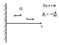
Figure 1: For a particle Q free to move in a semi-space, bounded by a rigid wall located at $x=0$, the operator $-i\partial/\partial x$ has the clear physical meaning of the particle momentum $x$-component even if it is not selfadjoint (cf. von Neumann[45], and Refs.[8, 9]): See the text.

At this point, let us emphasize that our previously assumed boundary condition $E\neq 0$ can be dispensed with, by having recourse [3, 4, 8, 9] to the bi-linear hermitian operator

$$\hat{t}=\displaystyle\frac{-i\hbar}{2}\displaystyle\frac{\stackrel{{\scriptstyle\leftrightarrow}}{{\partial}}}{\partial E}$$ (10)

where the meaning of the sign $\leftrightarrow$ is clear from the accompanying definition

$$(f,\,\hat{t}\,g)=\Bigl{(}f,\>-\displaystyle\frac{ih}{2}\displaystyle\frac{\partial}{\partial E}\,g\Bigr{)}+\Bigl{(}-\displaystyle\frac{ih}{2}\,\displaystyle\frac{\partial}{\partial E}\,f,\;g\Bigr{)}\,.$$

By adopting this expression for the time operator, the algebraic sum of the two terms in the r.h.s. of the last relation results to be automatically zero at point $E=0$. This question will be exploited below, in Sect. 3 (when dealing with the more general case of the four-position operator). Incidentally, such an “elimination” [8, 9, 3, 4] of point $E=0$ is not only simpler, but also more physical, than other kinds of elimination obtained much later in papers like [33, 34].

In connection with the last quotation, leu us for briefly comment on the so-called positive-operator-value-measure (POVM) approach, often used or discussed in the second set of papers on time in quantum physics mentioned in our Introduction. Actually, an analogous procedure had been proposed, since the sixties [46], in some approaches to the quantum theory of measurements. Afterwards, and much later, the POVM approach has been applied, in a simplified and shortened form, to the time-operator problem in the case of one-dimensional free motion: for instance, in Refs.[16,18,21,29-37] and especially in [33, 34]. These papers stated that a generalized decomposition of unity (or “POV measure”) could be obtained from selfadjoint extensions of the time operator inside an extended Hilbert space (for instance, adding the negative values of the energy, too), by exploiting the Naimark dilation-theorem[47]: But such a program has been realized till now only in the simple cases of one-dimensional particle free motion.

By contrast, our approach is based on a different Naimark’s theorem[39], which, as already mentioned above, allows a much more direct, simple and general –and at the same time non less rigorous– introduction of a quantum operator for Time.  More precisely, our approach is based on the so-called Carleman theorem[48], utilized in Ref.[39], about approximating a hermitian operator by suitable successions of “bounded” selfadjoint operators: That is, of selfadjoint operators whose spectral functions do weakly converge to the non-orthogonal spectral function of the considered hemitian operator.  And our approach is applicable to a large family of three-dimensional (3D) particle collisions, with all possible Hamiltonians. Actually, our approach was proposed in the early Refs.[3-10] and in Ref.[24], and applied therein for the time analyzis of quantum collisions, nuclear reactions and tunnelling processes.

2.2 On the momentum representation of the Time operator

In the continuous spectrum case, instead of the $E$-representation, with $0<E<+\infty$, in Eqs.(1)–(4) one can also use the $k$-representation[14, 15], with the advantage that $-\infty<k<+\infty$:

$$\Psi\,(x,t)=\displaystyle\int\limits_{-\infty}^{+\infty}g(k)\,\varphi(x,k)\,\exp(-iEt/\hbar)\>dk$$ (11)

with $E=\hbar^{2}k^{2}/\,2\mu$, and $k\neq 0$.

For the extension of the momentum representation to the case of $\langle t^{n}\rangle$, with $n>1$, we confine ourselves here to refer the reader to the papers [27, 41, 38].

2.3 An alternative weight for time averages (in the cases of particle dwelling inside a certain spatial region)

We recall that the weight (2) [as well as its modifications (3)] has the meaning of a probability for the considered particle to pass through point $x$ during the time interval ($t$, $t+dt$). Let us follow the procedure presented in Refs.[24, 25, 28, 26, 27] and refs. therein, and analyze the consequences of the equality

$$\int\limits_{-\infty}^{+\infty}j\,(x,t)\>dt=\displaystyle\int\limits_{-\infty}^{+\infty}\bigl{|}\,\Psi(x,t)\bigr{|}^{2}\>dx$$ (12)

obtained from the 1D continuity equation. One can easily realize that a second, alternative weight can be adopted:

$$d\,P(x,t)\equiv Z\,(x,t)\>dx=\displaystyle\frac{\bigl{|}\Psi(x,t)\bigr{|}^{2}\>dx}{\displaystyle\int\limits_{-\infty}^{+\infty}\bigl{|}\,\Psi(x,t)\bigr{|}^{2}\>dx}$$ (13)

which possesses the meaning of probability for the particle to be located (or to sojourn, i. e., to dwell) inside the infinitesimal space region ($x$, $x+dx$) at the instant $t$, independently of its motion properties. Then, the quantity

$$P(x_{1},x_{2},t)=\displaystyle\frac{\displaystyle\int\limits_{x_{1}}^{x_{2}}\bigl{|}\Psi(x,t)\bigr{|}^{2}\>dx}{\displaystyle\int\limits_{-\infty}^{+\infty}\bigl{|}\,\Psi(x,t)\bigr{|}^{2}\>dx}$$ (14)

will have the meaning of probability for the particle to dwell inside the spatial interval ($x_{1}$, $x_{2}$) at the instant $t$.

As it is known (see, for instance, Refs.[24, 25, 26, 27, 38] and refs. therein), the mean dwell time can be written in the two equivalent forms:

$$\langle\tau(x_{i},x_{f})\rangle=\displaystyle\frac{\displaystyle\int\limits_{-\infty}^{+\infty}dt\ \displaystyle\int\limits_{x_{i}}^{x_{f}}|\Psi(x,t)|^{2}\;dx}{\displaystyle\int\limits_{-\infty}^{+\infty}j_{\rm in}(x_{i},t)\;dt}$$ (15)

and

$$\langle\tau(x_{i},x_{f})\rangle=\displaystyle\frac{\displaystyle\int\limits_{-\infty}^{+\infty}t\,j(x_{f},t)\;dt-\displaystyle\int\limits_{-\infty}^{+\infty}t\,j(x_{i},t)\;dt}{\displaystyle\int\limits_{-\infty}^{+\infty}j_{\rm in}(x_{i},t)\;dt}\;,$$ (16)

where it has been taken account, in particular, of relation (12), which follows — as already said — from the continuity equation.

Thus, in correspondence with the two measures (2) and (13), when integrating over time one gets two different kinds of time distributions (mean values, variances…), which refer to the particle traversal time in the case of measure (2), and to the particle dwelling in the case of measure (13). Some examples for 1D tunneling are contained in Refs.[24-27].

2.4 Time as a quantum-theoretical Observable in the case of Photons

As is known (see, for instance, Refs.[49, 50, 26]), in first quantization the single-photon wave function can be probabilistically described in the 1D case by the wave-packet

$${\mbox{\boldmath$A$}}({\mbox{\boldmath$r$}},t)=\displaystyle\int\limits_{k_{0}}\displaystyle\frac{d^{3}k}{k_{0}}\;{\mbox{\boldmath$\chi$}}({\mbox{\boldmath$k$}})\>\varphi({\mbox{\boldmath$k$}},{\mbox{\boldmath$r$}})\>\exp(-ik_{0}t)\;,$$ (17)

where, as usual, ${\mbox{\boldmath$A$}}({\mbox{\boldmath$r$}},t)$ is the electromagnetic vector potential, while ${\mbox{\boldmath$r$}}=\{x,y,z\}$,  ${\mbox{\boldmath$k$}}=\{k_{x},k_{y},k_{z}\}$,  $k_{0}\equiv w/c=\varepsilon/\,\hbar c$, and $k\equiv|{\mbox{\boldmath$k$}}|=k_{0}$. The axis $x$ has been chosen as the propagation direction. Let us notice that ${\mbox{\boldmath$\chi$}}({\mbox{\boldmath$k$}})=\sum\limits_{i=y,z}\chi_{i}({\mbox{\boldmath$k$}})\,{\mbox{\boldmath$e$}}_{i}({\mbox{\boldmath$k$}})$,  with  ${\mbox{\boldmath$e$}}_{i}{\mbox{\boldmath$e$}}_{j}=\delta_{ij}$, and $x_{i},x_{j}=y,z$, while $\chi_{i}({\mbox{\boldmath$k$}})$ is the probability amplitude for the photon to have momentum $k$ and polarization ${\mbox{\boldmath$e$}}_{j}$ along $x_{j}$. Moreover, it is $\varphi({\mbox{\boldmath$k$}},{\mbox{\boldmath$r$}})=\exp(ik_{x}x)$ in the case of plane waves, while $\varphi({\mbox{\boldmath$k$}},{\mbox{\boldmath$r$}})$ is a linear combination of evanescent (decreasing) and anti-evanescent (increasing) waves in the case of “photon barriers” (i.e., band-gap filters, or even undersized segments of waveguides for microwaves, or frustrated total-internal-reflection regions for light, and so on). Although it is not easy to localize a photon in the direction of its polarization[49, 50], nevertheless for 1D propagations it is possible to use the space-time probabilistic interpretation of Eq.(17), and define the quantity

$$\begin{array}[]{cc}\rho_{\rm em}(x,t)\>dx=\displaystyle\frac{S_{0}\>dx}{\int S_{0}\>dx},&S_{0}=\displaystyle\int\displaystyle\int s_{0}\>dy\,dz\end{array}$$ (18)

($s_{0}=[{\mbox{\boldmath$E$}}^{*}\cdot{\mbox{\boldmath$E$}}+{\mbox{\boldmath$H$}}^{*}\cdot{\mbox{\boldmath$H$}}]/\,4\pi$ being the energy density, with the electromagnetic field ${\mbox{\boldmath$H$}}={\rm rot}\,{\mbox{\boldmath$A$}}$,  and  $\mbox{\boldmath$E$}=-1/c\;\partial{\mbox{\boldmath$A$}}/\partial t$), which represents the probability density of a photon to be found (localized) in the spatial interval ($x$, $x+dx$) along the $x$-axis at the instant $t$;  and the quantity

$$\begin{array}[]{cc}j_{\rm em}(x,t)\>dt=\displaystyle\frac{S_{x}\>dt}{\int S_{x}(x,t)\>dt},&S_{x}(x,t)=\displaystyle\int\displaystyle\int s_{x}\>dy\,dz\end{array}$$ (19)

($s_{x}=c\;\Re[{\mbox{\boldmath$E$}}^{*}\wedge{\mbox{\boldmath$H$}}]_{x}\,/\>8\pi$ being the energy flux density), which represents the flux probability density of a photon to pass through point $x$ in the time interval ($t$, $t+dt$): in full analogy with the probabilistic quantities for non-relativistic particles. The justification and convenience of such definitions is self-evident, when the wave-packet group velocity coincides with the velocity of the energy transport;  in particular:  (i) the wave-packet (17) is quite similar to wave-packets for non-relativistic particles,  and  (ii) in analogy with conventional non-relativistic quantum mechanics, one can define the “mean time instant” for a photon (i.e., an electromagnetic wave-packet) to pass through point $x$, as follows

$$\langle t(x)\rangle=\displaystyle\int\limits_{-\infty}^{+\infty}t\,J_{{\rm em},\,x}\;dt=\displaystyle\frac{\displaystyle\int\limits_{-\infty}^{+\infty}t\,S_{x}(x,t)\;dt}{\displaystyle\int\limits_{-\infty}^{+\infty}S_{x}(x,t)\;dt}\;.$$

As a consequence [in the same way as in the case of equations (1)–(2)], the form (1) for the time operator in the energy representation is valid also for photons, with the same boundary conditions adopted in the case of particles, that is, with $\chi_{i}\,(0)=\chi_{i}\,(\infty)$ and with $E=\hbar\,c\,k_{0}$.

The energy density $s_{0}$ and energy flux density $s_{x}$ satisfy the relevant continuity equation

$$\frac{\partial s_{0}}{\partial t}+\displaystyle\frac{\partial s_{x}}{\partial x}=0$$ (20)

which is Lorentz-invariant for 1D spatial propagation[26, 27, 38] processes.

2.5 Introducing the analogue of the “Hamiltonian” for the case of the Time operator: A new hamiltonian approach

In non-relativistic quantum theory, the Energy operator acquires (cf., e.g., Refs.[11-13,27,38]) the two forms:  (i)  $i\hbar\,\displaystyle\frac{\partial}{\partial t}$ in the $t$-representation, and  (ii)  $\hat{H}\,(\hat{p}_{x},\hat{x},\ldots)$ in the hamiltonianian formalism. The “duality” of these two forms can be easily inferred from the Schröedinger equation itself,  $\hat{H}\Psi=i\hbar\displaystyle\frac{\partial\Psi}{\partial t}$. One can introduce in quantum mechanics a similar duality for the case of Time: Besides the general form (1) for the Time operator in the energy representation, which is valid for any physical systems in the region of continuous energy spectra, one can express the time operator also in a “hamiltonian form”, i.e., in terms of the coordinate and momentum operators, by having recourse to their commutation relations.  Thus, by the replacements

$$\begin{array}[]{c}\vspace{3mm}\hat{E}\to\hat{H}\,(\hat{p}_{x},\hat{x},\ldots),\\ \hat{t}\to\hat{T}\,(\hat{p}_{x},\hat{x},\ldots),\end{array}$$ (21)

and on using the commutation relation [similar to Eq.(3)]

$$[\hat{H},\,\hat{T}]=i\hbar\;,$$ (22)

one can obtain[51], given a specific ordinary Hamiltonian, the corresponding explicit expression for $\hat{T}\,(\hat{p}_{x},\hat{x},\ldots)$.

Indeed, this procedure can be adopted for any physical system with a known Hamiltonian $\hat{H}\,(\hat{p}_{x},\hat{x},\ldots)$, and we are going to see a concrete example. By going on from the coordinate to the momentum representation, one realizes that the formal expressions of both the hamiltonian-type operators $\hat{H}\,(\hat{p}_{x},\hat{x},\ldots)$ and $\hat{T}\,(\hat{p}_{x},\hat{x},\ldots)$ do not change, except for an obvious change of sign in the case of operator $\hat{T}\,(\hat{p}_{x},\hat{x},\ldots)$.

As an explicit example, let us address the simple case of a free particle whose Hamiltonian is

$$\hat{H}=\left\{\begin{array}[]{ccll}\hat{p}_{x}^{2}/\,2\mu,&\hat{p}_{x}=-i\hbar\displaystyle\frac{\partial}{\partial x}\,,&\mbox{ \ \ \ \ in the coordinate representation}&\mbox{(a)}\\ p_{x}^{2}/\,2\mu\,.&&\mbox{ \ \ \ \ in the momentum representation}&\mbox{(a)}\end{array}\right.$$ (23)

Correspondingly, the Hamilton-type time operator, in its symmetrized form, will write

$$\hat{T}=\left\{\begin{array}[]{clll}\vspace{2mm}\displaystyle\frac{\mu}{2}\,\Bigl{(}\hat{p}_{x}^{-1}x+x\hat{p}_{x}^{-1}+i\hbar\,;\ \hat{p}_{x}^{-2}\Bigr{)},&{\rm in\ the\ coordinate\ representation}&\mbox{(a)}\\ -\displaystyle\frac{\mu}{2}\,\Bigl{(}p_{x}^{-1}\hat{x}+\hat{x}p_{x}^{-1}+i\hbar/p_{x}^{2}\Bigr{)},&{\rm in\ the\ momentum\ representation}&\mbox{(b)}\end{array}\right.$$ (24)

where

$$\begin{array}[]{cc}\hat{p}_{x}^{-1}=\displaystyle\frac{i}{\hbar}\int dx\ldots,&\hskip 19.91692pt\hat{x}=i\hbar\displaystyle\frac{\partial}{\partial p_{x}}\;.\end{array}$$

Incidentally, operator (24b) is equivalent to $-i\hbar\,\frac{\partial}{\partial E}$, since $E=p_{x}^{2}/\,2\mu$; and therefore it is also a (maximal) hermitian operator. Indeed, by applying the operator $\hat{T}\,(\hat{p}_{x},\hat{x},\ldots)$, for instance, to a plane-wave of the type $\exp(ikx)$, we obtain the same result in both the coordinate and the momentum representations:

$$\hat{T}\;\exp(ikx)=\displaystyle\frac{x}{v}\>\exp(ikx)$$ (25)

quantity ${x}/{v}$ being the free-motion time (for a particle with velocity $v$ ) for traveling the distance $x$.

On the basis of what precedes, it is possible to show that the wave function $\Psi(x,t)$ of a quantum system satisfies the two (dual) equations

$$\begin{array}[]{ccc}\hat{H}\,\Psi=i\hbar\displaystyle\frac{\partial\Psi}{\partial t}&\mbox{and}&\hat{T}\,\Psi=t\,\Psi\,.\end{array}$$ (26)

In the energy representation, and in the stationary case, we obtain again two (dual) equations

$$\begin{array}[]{ccc}\hat{H}\,\varphi_{t}=\varepsilon\,\varphi_{t}&\mbox{and}&\hat{T}\,\varphi_{t}=-i\hbar\displaystyle\frac{\partial\varphi_{t}}{\partial\varepsilon}\;,\end{array}$$ (27)

quantity $\varphi_{t}$ being the Fourier-transform of $\Psi$:

$$\varphi_{t}=\displaystyle\frac{1}{2\pi\hbar}\displaystyle\int\limits_{-\infty}^{+\infty}\Psi(x,t)\>e^{i\varepsilon t/\hbar}\;dt\,.$$ (28)

It might be interesting to apply the two pairs of the last dual equations also for investigating tunnelling processes through the quantum gravitational barrier, which appears during inflation, or at the beginning of the big-bang expansion, whenever a quasi-linear Schrödinger-type equation does approximately show up.

2.6 Time as an Observable (and the Time-Energy uncertainty relation), for quantum-mechanical systems with discrete energy spectra

For describing the time evolution of non-relativistic quantum systems endowed with a purely discrete (or a continuous and discrete) spectrum, let us now introduce wave-packets of the form [11, 12, 13, 27, 41, 38]:

$$\psi\,(x,t)=\sum\limits_{n=0}g_{n}\,\varphi_{n}(x)\,\exp[-i(\varepsilon_{n}-\varepsilon_{0})t/\hbar]\;,$$ (29)

where $\varphi_{n}(x)$ are orthogonal and normalized bound states which satisfy the equation $\hat{H}\,\varphi_{n}(x)=\varepsilon_{n}\,\varphi_{n}(x)$, quantity $\hat{H}$ being the Hamiltonian of the system; while the coefficients $g_{n}$ are normalized: $\sum\limits_{n=0}|g_{n}|^{2}=1$. We omitted the non-significant phase factor $\exp(-i\varepsilon_{0}t/\hbar)$ of the fundamental state.

Let us first consider the systems whose energy levels are separated by intervals admitting a maximum common divisor $D$ (for ex., harmonic oscillator, particle in a rigid box, and spherical spinning top), so that the wave packet (29) is a periodic function of time possessing as period the Poincaré cycle time $T=2\pi\hbar/D$. For such systems it is possible [11-13,27,41] to construct a selfadjoint time operator with the form (in the time representation) of a saw-function of $t$, choosing $t=0$ as the initial time instant:

$$\hat{t}\;=\;t-T\sum_{n=0}^{\infty}\Theta(t-[2n+1]T/2)+T\sum_{n=0}^{\infty}\Theta(-t-[2n+1]T/2\;.$$ (30)

This periodic function for the time operator is a linear (increasing) function of time $t$ within each Poincar cycle: Cf., e.g., figure 2 in Ref.[38], where the periodic saw-tooth function for the time operator, in the present case of quantum mechanical systems with discrete energy spectra [that is, of Eq.(30)], is explicitly shown.

The commutation relations of the Energy and Time operators, now both selfajoint, acquires in the case of discrete energies and of a periodic Time operator the form

$$[\hat{E},\hat{t}]\;=\;i\hbar\left\{1-T\sum_{n=0}^{\infty}\delta(t-[2n+1]T)\right\}\,,$$ (31)

wherefrom the uncertainty relation follows in the new form

$$(\Delta E)^{2}\;(\Delta t)^{2}\;=\;\hbar^{2}\left[1-{{T|\psi(T/2+\gamma)|^{2}}\over{\int_{-T/2}^{T/2}|\psi(t)|^{2}dt}}\right]\;,$$ (32)

where it has been introduced a parameter $\gamma$, with $-T/2<\gamma<T/2$, in order to assure that the r.h.s. integral is single-valued[27, 41].

When $\Delta E\rightarrow 0$ (that is, when $|g_{n}|\rightarrow\delta_{nn^{\prime}})$, the r.h.s. of Eq.(32) tends to zero too, since $|\psi(t)|^{2}$ tends to a constant value. In such a case, the distribution of the time instants at which the wave-packet passes through point $x$ becomes flat within each Poincaré cycle. When, by contrast, $\Delta E>>D$ and  $|\psi(T+\gamma)|^{2}<<(\int_{-T/2}^{T/2}|\psi(t)|^{2}dt)/T$, the periodicity condition may become inessential whenever $\Delta t<<t$. In other words, our uncertainty relation (32) transforms into the ordinary uncertainty relation for systems with continuous spectra.

In more general cases, for excited states of nuclei, atoms and molecules, the energy-level intervals, for discrete and quasi-discrete (resonance) spectra, are not multiples of a maximum common divisor, and hence the Poincaré cycle is not well-defined for such systems.  Nevertheless, even for those systems one can introduce an approximate description (sometimes, with any desired degree of accuracy) in terms of Poincaré quasi-cycles and a quasi-periodical evolution; so that for sufficiently long time intervals the behavior of the wave-packets can be associated with a a periodical motion (oscillation), sometimes — e.g., for very narrow resonances — with any desired accuracy. For them, when choosing an approximate Poincaré-cycle time, one can include in one cycle as many quasi-cycles as it is necessary for the demanded accuracy. Then, with the chosen accuracy, a quasi-selfadjoint time operator can be introduced.

3 On four-position operators in quantum field theory, in terms of bilinear operators

In this Section we approach the relativistic case, taking into consideration — therefore — the space-time (four-dimensional) “position” operator, starting however with an analysis of the 3-dimensional (spatial) position operator in the simple relativistic case of the Klein-Gordon equation. Actually, this analysis will lead us to tackle already with non-hermitian operators.  Moreover, while performing it, we shall meet the opportunity of introducing bilinear operators, which will be used even more in the next case of the full 4-position operator.

Let us recall that in Sect.2.1 we mentioned that the boundary condition $E\neq 0$, therein imposed to guarantee (maximal) hermiticity of the time operator, can be dispensed with just by having recourse to bilinear forms.  Namely, by considering the bilinear hermitian operator[8, 9, 40]  $\hat{t}=(-i\hbar\;{\stackrel{{\scriptstyle\leftrightarrow}}{{\partial}}}/{\partial E})/2$,  where the sign $\leftrightarrow$ is defined through the accompanying equality  $(f,\,\hat{t}\,g)=\Bigl{(}f,\>-\frac{ih}{2}\frac{\partial}{\partial E}\,g\Bigr{)}+\Bigl{(}-\frac{ih}{2}\,\frac{\partial}{\partial E}\,f,\;g\Bigr{)}$.

3.1 The Klein-Gordon case: Three-position operators

The standard position operators, being hermitian and moreover selfadjoint, are known to possess real eigenvalues: i.e., they yield a point-like localization. J. M. Jauch showed, however, that a point-like localization would be in contrast with “unimodularity”. In the relativistic case, moreover, phenomena so as the pair production forbid a localization with precision better than one Compton wave-length. The eigenvalues of a realistic position operator ${\hat{\mbox{\boldmath$z$}}}$ are therefore expected to represent space regions, rather than points. This can be obtained only by having recourse to non-hermitian (and therefore non-selfadjoint) position operators ${\hat{\mbox{\boldmath$z$}}}$ (a priori, one can have recourse either to non-normal operators with commuting components, or to normal operators with non-commuting components). Following, e.g., the ideas in Refs.[52-56], we are going to show that the mean values of the hermitian (selfadjoint) part of ${\hat{\mbox{\boldmath$z$}}}$ will yield a mean (point-like) position [57, 58], while the mean values of the anti-hermitian (anti-selfadjoint) part of ${\hat{\mbox{\boldmath$z$}}}$ will yield the sizes of the localization region[3, 4].

Let us consider, e.g., the case of relativistic spin-zero particles, in natural units and with metric $(+\,-\,-\,-)$. The position operator $i\,\nabla_{\mbox{\boldmath$p$}}$, is known to be actually non-hermitian, and may be in itself a good candidate for an extended-type position operator. To show this, we want to split[52-56] it into its hermitian and anti-hermitian (or skew-hermitian) parts.

Consider, then, a vector space $V$ of complex differentiable functions on a 3-dimensional phase-space[40] equipped with an inner product defined by

$$(\Psi,\,\Phi)=\displaystyle\int\displaystyle\frac{d^{3}{\mbox{\boldmath$p$}}}{p_{0}}\;\Psi^{*}({\mbox{\boldmath$p$}})\,\Phi(p)$$ (33)

quantity $p_{0}$ being $\sqrt{{\mbox{\boldmath$p$}^{2}}+m_{0}^{2}}$. Let the functions in $V$ satisfy moreover the condition

$$\lim\limits_{R\to\infty}\displaystyle\int\limits_{S_{R}}\displaystyle\frac{dS}{p_{0}}\;\Psi^{*}(p)\,\Phi(p)=0$$ (34)

where the integral is taken over the surface of a sphere of radius $R$.  If $U:V\to V$ is a differential operator of degree one, condition (34) allows a definition of the transpose $U^{T}$ by

$$\begin{array}[]{ccc}(U^{T}\Psi,\,\Phi)=(\Psi,\,U\,\Phi)&\mbox{for all }\Psi,\,\Phi\in V\;,\end{array}$$ (35)

where $U$ is changed into $U^{T}$, or vice-versa, by means of integration by parts.

This allows, further, to introduce a dual representation[40] ($U_{1}$, $U_{2}$) of a single operator $U_{1}^{T}+U_{2}$ by

$$(U_{1}\Psi,\,\Phi)+(\Psi,\,U_{2}\Phi)=(\Psi,\,(U_{1}^{T}+U_{2})\,\Phi).$$ (36)

With such a dual representation, it is easy to split any operator into its hermitian and anti-hermitian parts

$$(\Psi,\,U\Phi)=\displaystyle\frac{1}{2}\,\Bigl{(}(\Psi,\,U\Phi)+(U^{*}\Psi,\,\Phi)\Bigr{)}+\displaystyle\frac{1}{2}\,\Bigl{(}(\Psi,\,U\Phi)-(U^{*}\Psi,\,\Phi)\Bigr{)}.$$ (37)

Here the pair

$$\frac{1}{2}\,(U^{*},\,U)\equiv\,\stackrel{{\scriptstyle\leftrightarrow}}{{U}}_{h}\;,$$ (38)

corresponding to $(1/2)\,(U+U^{*T})$, represents the hermitian part, while

$$\frac{1}{2}(-U^{*},\,U)\equiv\,\stackrel{{\scriptstyle\leftrightarrow}}{{U}}_{a}$$ (39)

represents the anti-hermitian part.

Let us apply what precedes to the case of the Klein-Gordon position-operator $\hat{z}=i\,\nabla_{p}$. When

$$U=i\,\displaystyle\frac{\partial}{\partial p_{j}}$$ (40)

we have[3, 4]

$$\begin{array}[]{cl}\vspace{2mm}\displaystyle\frac{1}{2}\,(U^{*},\,U)=\displaystyle\frac{1}{2}\,\biggl{(}-i\,\displaystyle\frac{\partial}{\partial p_{j}},\,i\,\displaystyle\frac{\partial}{\partial p_{j}}\biggr{)}\equiv\,\displaystyle\frac{i}{2}\,\displaystyle\frac{\stackrel{{\scriptstyle\leftrightarrow}}{{\partial}}}{\partial p_{j}},&(a)\\ \displaystyle\frac{1}{2}\,(-U^{*},\,U)=\displaystyle\frac{1}{2}\,\biggl{(}i\,\displaystyle\frac{\partial}{\partial p_{j}},\,i\,\displaystyle\frac{\partial}{\partial p_{j}}\biggr{)}\equiv\,\displaystyle\frac{i}{2}\,\displaystyle\frac{\stackrel{{\scriptstyle\leftrightarrow}}{{\partial}}_{+}}{\partial p_{j}}.&(b)\end{array}$$ (41)

And the corresponding single operators turn out to be

$$\begin{array}[]{ll}\vspace{2mm}\displaystyle\frac{1}{2}\,(U+U^{*T})=i\,\displaystyle\frac{\partial}{\partial p_{j}}-\displaystyle\frac{i}{2}\,\displaystyle\frac{p_{j}}{p^{2}+m_{0}^{2}},&(a)\\ \displaystyle\frac{1}{2}\,(U-U^{*T})=\displaystyle\frac{i}{2}\,\displaystyle\frac{p_{j}}{p^{2}+m_{0}^{2}}\;.&(b)\end{array}$$ (42)

It is noteworthy[3, 4] that, as we are going to see, operator (42a) is nothing but the usual Newton-Wigner operator, while (42b) can be interpreted[52-56,3,4,31] as yielding the sizes of the localization-region (an ellipsoid) via its average values over the considered wave-packet.

Let us underline that the previous formalism justifies from the mathematical point of view the treatment presented in papers like [52-58].  We can split[3, 4] the operator $\hat{z}$ into two bilinear parts, as follows:

$$\hat{z}=i\,\nabla_{p}=\displaystyle\frac{i}{2}\,\stackrel{{\scriptstyle\leftrightarrow}}{{\nabla}}_{p}+\displaystyle\frac{i}{2}\,\stackrel{{\scriptstyle\leftrightarrow}}{{\nabla}}_{p}^{(+)}$$ (43)

where  $\Psi^{*}\stackrel{{\scriptstyle\leftrightarrow}}{{\nabla}}_{p}\Phi\equiv\,\Psi^{*}\nabla_{p}\Phi-\Phi\nabla_{p}\Psi^{*}$  and  $\Psi^{*}\stackrel{{\scriptstyle\leftrightarrow}}{{\nabla}}_{p}^{(+)}\Phi\equiv\,\Psi^{*}\nabla_{p}\Phi+\Phi\nabla_{p}\Psi^{*}\,,$ and where we always referred to a suitable[52-58,8,9,40] space of wave packets. Its hermitian part[52-58]

$$\hat{x}=\displaystyle\frac{i}{2}\,\stackrel{{\scriptstyle\leftrightarrow}}{{\nabla}}_{p}\;,$$ (44)

which was expected to yield an (ordinary) point-like localization, has been derived also by writing explicitly

$$(\Psi,\,\hat{x}\,\Phi)=i\,\displaystyle\int\displaystyle\frac{d^{3}p}{p_{0}}\;\Psi^{*}(p)\,\nabla_{p}\,\Phi(p)$$ (45)

and imposing hermiticity, i.e., imposing the reality of the diagonal elements. The calculations yield

$$\Re\,\bigl{(}\Phi,\,\hat{x}\,\Phi\bigr{)}=i\,\displaystyle\int\displaystyle\frac{d^{3}p}{p_{0}}\;\Phi^{*}(p)\,\stackrel{{\scriptstyle\leftrightarrow}}{{\nabla}}_{p}\,\Phi(p)\;,$$ (46)

suggesting to adopt just the Lorentz-invariant quantity (44) as a bilinear hermitian position operator.  Then, on integrating by parts (and due to the vanishing of the surface integral), we verify that eq.(44) is equivalent to the ordinary Newton-Wigner operator:

$$\hat{x}_{h}\equiv\,\displaystyle\frac{i}{2}\,\stackrel{{\scriptstyle\leftrightarrow}}{{\nabla}}_{p}\>\equiv\,i\,\nabla_{p}-\displaystyle\frac{i}{2}\,\displaystyle\frac{{\mbox{\boldmath$p$}}}{p^{2}+m^{2}}\;\equiv{\rm N-W}\,.$$ (47)

We are left with the (bilinear) anti-hermitian part

$$\hat{y}=\displaystyle\frac{i}{2}\,\stackrel{{\scriptstyle\leftrightarrow}}{{\nabla}}_{p}^{(+)}$$ (48)

whose average values over the considered state (wave-packet) can be regarded as yielding[52-58,8,9,40] the sizes of an ellipsoidal localization-region.

After the digression associated with Eqs.(43)–(48), let us go back to the present formalism, as expressed by Eqs.(33)–(42).

In general, the extended-type position operator $\hat{z}$ will yeld

$$\langle\Psi|\,\hat{z}\,|\Psi\rangle=(\alpha+\Delta\alpha)+i\,(\beta+\Delta\beta)\;,$$ (49)

where $\Delta\alpha$ and $\Delta\beta$ are the mean-errors encountered when measuring the point-like position and the sizes of the localization region, respectively. It is interesting to evaluate the commutators ($i,j=1,2,3$):

$$\biggl{(}\displaystyle\frac{i}{2}\,\displaystyle\frac{\stackrel{{\scriptstyle\leftrightarrow}}{{\partial}}}{\partial p_{i}},\,\displaystyle\frac{i}{2}\,\displaystyle\frac{\stackrel{{\scriptstyle\leftrightarrow}}{{\partial}}_{(+)}}{\partial p_{j}}\biggr{)}=\displaystyle\frac{i}{2\,p_{0}^{2}}\,\biggl{(}\delta_{ij}-\displaystyle\frac{2\,p_{i}p_{j}}{p_{0}^{2}}\biggr{)}\,,$$ (50)

wherefrom the noticeable “uncertainty correlations” follow:

$$\Delta\alpha_{i}\ \Delta\beta_{j}\geq\displaystyle\frac{1}{4}\;\biggl{|}\biggl{\langle}\displaystyle\frac{1}{p_{0}^{2}}\;\biggl{(}\delta_{ij}-\displaystyle\frac{2\,p_{i}p_{j}}{p_{0}^{2}}\biggr{)}\biggr{\rangle}\biggr{|}\,.$$ (51)

3.2 Four-position operators

It is tempting to propose as four-position operator the quantity $\hat{z}^{\mu}=\hat{x}^{\mu}+i\,\hat{y}^{\mu}$, whose hermitian (Lorentz-covariant) part can be written

$$\hat{x}^{\mu}=-\,\displaystyle\frac{i}{2}\,\displaystyle\frac{\stackrel{{\scriptstyle\leftrightarrow}}{{\partial}}}{\partial p_{\mu}}\;,$$ (52)

to be associated with its corresponding “operator” in four-momentum space

$$\hat{p}_{h}^{\mu}=+\>\displaystyle\frac{i}{2}\,\displaystyle\frac{\stackrel{{\scriptstyle\leftrightarrow}}{{\partial}}}{\partial x_{\mu}}\;.$$ (53)

Let us recall the proportionality between the 4-momentum operator and the 4-current density operator in the chronotopical space, and then underline the canonical correspondence (in the 4-position and 4-momentum spaces, respectively) between the “operators” (cf. the previous subsection):

$$\begin{array}[]{ll}\vspace{2mm}m_{0}\,\hat{\rho}\,\equiv\,\hat{p}_{0}=\displaystyle\frac{i}{2}\,\displaystyle\frac{\stackrel{{\scriptstyle\leftrightarrow}}{{\partial}}}{\partial t}&(a)\\ m_{0}\,\hat{{\mbox{\boldmath$j$}}}\,\equiv\,\hat{{\mbox{\boldmath$p$}}}=-\displaystyle\frac{i}{2}\,\displaystyle\frac{\stackrel{{\scriptstyle\leftrightarrow}}{{\partial}}}{\partial{\mbox{\boldmath$r$}}}\;,&(b)\end{array}$$ (54)

and the operators

$$\begin{array}[]{ll}\vspace{2mm}\hat{t}\,\equiv\,-\displaystyle\frac{i}{2}\,\displaystyle\frac{\stackrel{{\scriptstyle\leftrightarrow}}{{\partial}}}{\partial p_{0}}&(a)\\ \hat{{\mbox{\boldmath$x$}}}\,\equiv\,\displaystyle\frac{i}{2}\,\displaystyle\frac{\stackrel{{\scriptstyle\leftrightarrow}}{{\partial}}}{\partial{\mbox{\boldmath$p$}}}\;,&(b)\end{array}$$ (55)

where the four-position “operator” (55) can be considered as a 4-current density operator in the energy-impulse space.  Analogous considerations can be carried on for the anti-hermitian parts (see Ref.[4]).

Finally, by recalling the properties of the time operator as a maximal hermitian operator in the non-relativistic case (Sec.2.1), one can see that the relativistic time operator (55a) (for the Klein-Gordon case) is also a selfadjoint bilinear operator for the case of continuous energy spectra, and a (maximal) hermitian linear operator for free particles [due to the presence of the lower limit zero for the kinetic energy, or $m_{0}$ for the total energy].

4 Some considerations on non-hermitian Hamiltonians

As to the important issue of Unstable States, and of their association with quasi-hermitian hamiltonians, let us confine ourselves to refer the interested reader to Sect. 4 in Ref.[38], a Section based on previous work performed in collaboration with A. Agodi, M. Baldo, and A. Pennisi di Floristella.[59]

Here, we shall only mention the case of the nuclear optical model and of microscopic quantum dissipation, and deal with an approach to the measurement problem in QM in terms of the chronon.

Actually, we shall deal with the chronon formalism[73] —where the chronon $\tau_{0}$ is a “quantum” of time, in the sense specified below— non only for its obvious connection with our view of time, and of space-time, but also because that discrete formalism has a non-hermitian character, as stressed e.g. in the Appendices of Ref.[73]. For instance, in its Schrödinger representation (see the following), proper continuous equations can reproduce the outputs obtained with the discretized equations, once we replace the (discrete) conventional Hamiltonian by a suitable (continuous) non-hermitian Hamiltonian, that can be called the “equivalent Hamiltonian”.  One important point is that non-hermitian Hamiltonians imply non-unitary evolution operators…

4.1 Nuclear optical model

Since the fifties, the so-called optical model has been frequently used for describing the experimental data on nucleon-nucleus elastic scattering, and, not less, on more general nuclear collisions: see, e.g., Refs.[60-63]; while for a generalized optical model — namely, the coupled-channel method with an optical model in any channel of the nucleon-nucleus (elastic or inelastic) scattering, one can see Ref.[64] and refs. therein.

In those cases, the Hamiltonian contains a complex potential, its imaginary part describing the absorption processes that take place by compound-nucleus formation and subsequent decay. As to the Hamiltonian with complex potential, here we confine ourselves at referring to work of ours already published, where it was studied the non-unitarity and analytical structure of the $S$-matrix, the completeness of the wave-functions, and so on: see Ref.[65], and also [66, 67].

4.2 Microscopic quantum dissipation

Before going on, let us inform the interested reader that in the Appenxix to the already quoted Ref.[38] there can be found some discussions and details related to the time-dependent Schrödinger equation with dissipative terms.

Various different approached are known, aimed at getting dissipation — and possibly decoherence — within quantum mechanics. First of all, the simple introduction of a “chronon” (see, e.g., Refs.[68-73]) allows one to go on from differential to finite-difference equations, and in particular to write down the quantum theoretical equations (Schrödinger’s, Liouville-von Neumann’s, etc.) in three different ways: symmetrical, retarded, and advanced. The retarded “Schrödinger” equation describes in a rather simple and natural way a dissipative system, which exchanges (loses) energy with the environment. The corresponding non-unitary time-evolution operator obeys a semigroup law and refers to irreversible processes. The retarded approach furnishes, moreover, an interesting way for proceeding in the direction of solving the “measurement problem” in quantum mechanics, without any need for a wave-function collapse: see Refs.[78, 80, 81, 74, 73]. The chronon theory can be regarded as a peculiar “coarse grained” description of the time evolution.

Let us stress that it has been shown that the mentioned discrete approach can be replaced with a continuous one, at the price of introducing a non-hermitian Hamiltonian: see, e.g., Ref.[82].

Further relevant work can be found, for instance, in papers like [83-93] and refs. therein.

Let us add that much work is still needed, however, for the description of time irreversibility at the microscopic level. Indeed, various approaches have been proposed, in which new parameters are introduced (regulation or dissipation) into the microscopic dynamics (building a bridge, in a sense, between microscopic structure and macroscopic characteristics). Besides the Caldirola-Kanai[94, 95] Hamiltonian

$$\hat{H}_{{\rm CK}}(t)=-\,\displaystyle\frac{\hbar^{2}}{2m}\>\displaystyle\frac{\partial^{2}}{\partial x^{2}}e^{-\gamma t}+V(x)\;e^{\gamma t}$$ (56)

(which has been used, e.g., in Ref.[96]), other rather simple approaches, based of course on the Schrödinger equation

$$i\hbar\,\displaystyle\frac{\partial}{\partial t}\;\Psi(x,t)=\hat{H}\,\Psi(x,t)\,,$$ (57)

and adopting a microscopic dissipation defined via a coefficient of extinction $\gamma$, are known. In Sect.5 of Ref.[38] we gave some details on:  A) Non-Linear (non-hermitian) Hamiltonians, with “potential” operators of Kostin’s, Albrecht’s, and Hasse’s types;  and  B) Linear (non-hermitian) Hamiltonians, of Gisin’s, and Exner’s types.

One may here recall also the important, so-called “microscopic models”[97], even if they are not based on the Schröedinger equation.

All such proposals are to be further investigated, and completed, since till now they do not appear to have been exploited enough. Let us remark, just as an example, that it would be desirable to take into deeper consideration other related phenomena, like the ones associated with the “Hartman effect” (and “generalized Hartman effect”) [26, 24, 25, 98, 101, 100, 99], in the case of tunneling with dissipation: a topic faced in few papers, like [102, 103].

As already mentioned, in the Appendix to Ref.[38], we presented for example a scheme of iterations (successive approximations) as a possible tool for explicit calculations of wave-functions in the presence of dissipation.

At last, let us incidentally recall that two generalized Schröedinger equations, introduced by Caldirola [84, 104, 105, 106] in order to describe two different dissipative processes (behavior of open systems, and the radiation of a charged particle) have been shown — see, e.g., Ref.[107]) — to possess the same algebraic structure of the Lie-admissible type[109].

4.3 Approaching the “Measurement Problem” in QM in terms of a chronon $\tau_{0}$

In the previous subsection we already addressed Caldirola’s theory “of the Chronon”.

With that theory as inspiration, we wish now to present a simple quantum (finite difference) equation for dissipation and decoherence, on the basis of work performed in collaboration with R.H.A.Farias.[73, 74]

Namely, as said above, the mere introduction (not of a “time-lattice”, but simply) of a ‘chronon’ $\tau_{0}$ allows one to go on from differential to finite-difference equations; and in particular to write down the Schroedinger equation (as well as the Liouville–von Neumann equation) in three different ways: “retarded”, “symmetrical”, and “advanced”. One of such three formulations —the retarded one— describes in an elementary way a system which is exchanging (and losing) energy with the environment. In its density-matrix version, indeed, it can be easily shown that all non-diagonal terms go to zero very rapidly.

We already mentioned that we are interested in the chronon formalism[73] non only for its obvious connection with our view of time, and of space-time, but also because the discrete formalism has a non-hermitian character [as clarified e.g. in the Appendices of Ref.[73]]. For instance, in its Schrödinger representation (see the following), proper continuous equations can reproduce the outputs obtained with the discretized equations, once we replace the (discrete) conventional Hamiltonian by a suitable (continuous) non-hermitian Hamiltonian, that can be called the “equivalent Hamiltonian”. Indeed, in some special cases, the finite-difference equations can be solved by one of the (not easy) existing methods. An interesting alternative method is, however, finding out a new Hamiltonian $\tilde{H}$ such that the new continuous Schrödinger equation

$$i\hbar{{\partial\Psi\left({\bf x,t}\right)}\over{\partial t}}=\tilde{H}\Psi\left({\bf x,t}\right)$$

reproduces, at the points $t=n\tau_{0}$ (see below), the same results obtained from the discretized equations. As it was shown by Casagrande and Montaldi, it is always possible to find a continuous generating function which makes it possible to obtain a differential equation equivalent to the original finite-difference one, such that at every point of interest their solutions are identical [this procedure is useful since it is generally very difficult to work with the finite–difference equations on a qualitative basis; except for some very special cases, they can be only numerically solved]. This equivalent Hamiltonian $\tilde{H}$ is, however, non-hermitian and it is often quite difficult to be obtained: Happily enough, for the special case where the Hamiltonian is time independent, the equivalent Hamiltonian is quite easy to calculate. For example, in the symmetric equation case, it would be given by

$$\tilde{H}={\hbar\over\tau}\sin^{-1}({{\tau\over\hbar}\hat{H}}).$$

Of course,  $\tilde{H}\rightarrow\hat{H}$  when  $\tau_{0}\rightarrow 0$.

Since the introduction of the chronon has various consequences for Classical and Quantum Physics (also, as we have argued, for the decoherence problem), let us open a new Section about all that.

5 The particular case of the “Chronon”. Its consequences for Classical and Quantum Physics (and for Decoherence)

As we were saying, let us devote a brief Section to the consequence of the introduction of a Chronon for Classical Physics and for Quantum Mechanics (and for a new approach to Decoherence); without forgetting what stated in the previous two subsebsections. The consequences and applications of the “Chronon” are really various, an example being Ref.[114], where it was suggested that the chronon approach can account also for the origin of the internal degrees of freedom of the particles.  In the last subsection of this Section we shall mention with the possible role of the chronon in Cosmology.

Let us recall first of all that the interesting Caldirola’s “finite difference” theory forwards —at the classical level— a solution for the motion of a particle endowed with a non-negligible charge in an external electromagnetic field, overcoming all the known difficulties met by Abraham-Lorentz’s and Dirac’s approaches (and even allowing a clear answer to the question whether a free falling charged particle does or does not emit radiation), and —at the quantum level— yields a remarkable mass spectrum for leptons.

In Ref.[73] (where also extensive references can be found), after having reviewed Caldirola’s approach, we worked out, discussed, and compared to one another the new representations of Quantum Mechanics (QM) resulting from it, in the Schroedinger, Heisenberg and density-operator (Liouville–von Neumann) pictures, respectively.

For each representation, three (retarded, symmetric and advanced) formulations are possible, which refer either to times $t$ and $t-\tau_{0}$, or to times $t-\tau_{0}/2$ and $t+\tau_{0}/2$, or to times $t$ and $t+\tau_{0}$, respectively.  It is interesting to notice that, when the chronon tends to zero, the ordinary QM is obtained as the limiting case of the “symmetric” formulation only; while the “retarded” one does naturally appear to describe QM with friction, i.e., to describe dissipative quantum systems (like a particle moving in an absorbing medium). In this sense, discretized QM is much richer than the ordinary one.

In the mentioned work[73], we also obtained the (retarded) finite-difference Schroedinger equation within the Feynman path integral approach, and studied some of its relevant solutions. We have then derived the time-evolution operators of this discrete theory, and used them to get the finite-difference Heisenberg equations. [Afterward, we studied some typical applications and examples: as the free particle, the harmonic oscillator and the hydrogen atom; and various cases have been pointed out, for which the predictions of discrete QM differ from those expected from “continuous” QM].

We want to pay attention here to the fact that, when applying the density matrix formalism towards the solution of the measurement problem in QM, some interesting results are met, as, for instance, a possible, natural explication of the “decoherence”[74] due to dissipation: Which reveals some of the power of dicretized (in particular, retarded) QM.

5.1 Outline of the classical approach

If $\rho$ is the charge density of a particle on which an external electromagnetic field acts, the Lorentz’s force law

$$\bf{f}=\rho\left({\bf{E}+\frac{1}{c}\bf{v}\wedge\bf{B}}\right)\ ,$$

is valid only when the particle charge $q$ is negligible with respect to the external field sources. Otherwise, the classical problem of the motion of a (non-negligible) charge in an electromegnetic field is still an open question. For instance, after the known attempts by Abraham and Lorentz, in 1938 Dirac[75] obtained and proposed his known classical equation

$$m\frac{{\rm d}u_{\mu}}{{\rm d}s}=F_{\mu}+\Gamma_{\mu}\ ,$$ (58)

where $\Gamma_{\mu}$ is the Abraham 4-vector

$$\Gamma_{\mu}=\frac{2}{3}\frac{e^{2}}{c}\left({\frac{{\rm d}^{2}u_{\mu}}{{\rm d}s^{2}}+\frac{u_{\mu}u^{\nu}}{c^{2}}\frac{{\rm d}^{2}u_{\nu}}{{\rm d}s^{2}}}\right)\ ,$$ (59)

that is, the (Abraham) reaction force acting on the electron itself; and $F_{\mu}$ is the 4-vector that represents the external field acting on the particle

$$F_{\mu}=\frac{e}{c}F_{\mu\nu}u^{\nu}\ .$$ (60)

At the non-relativistic limit, Dirac’s equation goes formally into the one previously obtained by Abraham-Lorentz:

$$m_{0}\frac{{\rm d}{\bf v}}{{\rm d}t}-\frac{2}{3}\frac{e^{2}}{c^{3}}\frac{{\rm d}^{2}{\bf v}}{{\rm d}t^{2}}=e\left({{\bf E}+\frac{1}{c}{\bf v}\wedge{\bf B}}\right)\ .$$ (61)

The last equation shows that the reaction force equals  ${2\over 3}\;{e^{2}\over c^{3}}\;{{\rm d}^{2}{\bf v}\over{{\rm d}}t^{2}}$.

Dirac’s dynamical equation (58) is known to present, however, many troubles, related to the infinite many non-physical solutions that it possesses.  Actually, it is a third-order differential equation, requiring three initial conditions for singling out one of its solutions.  In the description of a free electron, e.g., it yields “self-accelerating” solutions (runaway solutions), for which velocity and acceleration increase spontaneously and indefinitely. Moreover, for an electron submitted to an electromagnetic pulse, further non-physical solutions appear, related this time to pre-accelerations: If the electron comes from infinity with a uniform velocity $v_{0}$ and, at a certain instant of time $t_{0}$, is submitted to an electromagnetic pulse, then it starts accelerating before $t_{0}$.  Drawbacks like these motivated further attempts to find out a coherent (not pointlike) model for the classical electron.

Considering elementary particles as points is probably the sin plaguing modern physics (a plague that, unsolved in classical physics, was transferred to quantum physics). One of the simplest way for associating a discreteness with elementary particles (let us consider, e.g., the electron) is just via the introduction (not of a “time-lattice”, but merely) of a “quantum” of time, the chronon, following Caldirola.[76]  Like Dirac’s, Caldirola’s theory is also Lorentz invariant (continuity, in fact, is not an assumption required by Lorentz invariance).  This theory postulates the existence of a universal interval $\tau_{0}$ of proper time, even if time flows continuously as in the ordinary theory. When an external force acts on the electron, however, the reaction of the particle to the applied force is not continuous: The value of the electron velocity $u_{\mu}$ is supposed to jump from $u_{\mu}(\tau-\tau_{0})$ to $u_{\mu}(\tau)$ only at certain positions $s_{n}$ along its world line; these “discrete positions” being such that the electron takes a time $\tau_{0}$ for travelling from one position $s_{\rm{n}-1}$ to the next one $s_{n}$.  The electron, in principle, is still considered as pointlike, but the Dirac relativistic equations for the classical radiating electron are replaced:  (i) by a corresponding finite–difference (retarded) equation in the velocity $u^{\mu}(\tau)$

$${{m_{0}}\over{\tau_{0}}}\left\{{u_{\mu}\left(\tau\right)-u_{\mu}\left({\tau-\tau_{0}}\right)+{{u_{\mu}\left(\tau\right)u_{\nu}\left(\tau\right)}\over{c^{2}}}\left[{u_{\nu}\left(\tau\right)-u_{\nu}\left({\tau-\tau_{0}}\right)}\right]}\right\}\ =$$

$$=\ {e\over c}F_{\mu\nu}\left(\tau\right)u_{\nu}\left(\tau\right),$$ (62)

which reduces to the Dirac equation (58) when $\tau_{0}\rightarrow 0$;  and  (ii) by a second equation [the transmission law] connecting this time the discrete positions $x^{\mu}(\tau)$ along the world line of the particle:

$x_{\mu}\left({n\tau_{0}}\right)-x_{\mu}\left[{\left({n-1}\right)\tau_{0}}\right]={{\tau_{0}}\over 2}\left\{{u_{\mu}\left({n\tau_{0}}\right)-u_{\mu}\left[{\left({n-1}\right)\tau_{0}}\right]}\right\},$ (62’)

which is valid inside each discrete interval $\tau_{0}$, and describes the internal motion of the electron.  In these equations, $u^{\mu}(\tau)$ is the ordinary four-vector velocity, satisfying the condition  $u_{\mu}(\tau)u^{\mu}(\tau)=-c^{2}$  for  $\tau=n\tau_{0}$,  where $n=0,1,2,...$  and  $\mu,\nu=0,1,2,3$;  while $F^{\mu\nu}$ is the external (retarded) electromagnetic field tensor,  and the chronon associated with the electron (by comparison with Dirac’s equation) resulted to be

${\tau_{0}\over 2}\equiv\theta_{0}={2\over 3}{{ke^{2}}\over{m_{0}c^{3}}}\simeq 6.266\times 10^{-24}\;{\rm s}\ ,$

depending, therefore, on the particle (internal) properties [namely, on its charge $e$ and rest mass $m_{0}$].

As a result, the electron happens to appear eventually as an extended–like[77] particle, with internal structure, rather than as a pointlike object. For instance, one may imagine that the particle does not react instantaneously to the action of an external force because of its finite extension (the numerical value of the chronon is of the same order as the time spent by light to travel along an electron classical diameter).  As already said, Eq.(62) describes the motion of an object that happens to be pointlike only at discrete positions $s_{n}$ along its trajectory; even if both position and velocity are still continuous and well-behaved functions of the parameter $\tau$, since they are differentiable functions of $\tau$. It is essential to notice that a discreteness character is given in this way to the electron without any need of a “model” for the electron. Actually it is well-known that many difficulties are met not only by the strictly pointlike models, but also by the extended-type particle models (“spheres”, “tops”, “gyroscopes”, etc.). We deem the answer stays with a third type of models, the “extended-like” ones, as the present approach; or as the (related) theories[77] in which the center of the pointlike charge is spatially distinct from the particle center-of-mass.  Let us repeat, anyway, that also the worst troubles met in quantum field theory, like the presence of divergencies, are due to the pointlike character still attributed to (spinning) particles; since —as we already remarked— the problem of a suitable model for elementary particles was transported, unsolved, from classical to quantum physics. One might say that problem to be the most important even in modern particle physics.

Equations (62) and the following one, together, provide a full description of the motion of the electron; but they are free from pre-accelerations, self-accelerating solutions, and problems with the hyperbolic motion.

In the non-relativistic limit the previous (retarded) equations get simplified, into the form

$${{m_{0}}\over{\tau_{0}}}\left[{{\bf v}\left(t\right)-{\bf v}\left({t-\tau_{0}}\right)}\right]=e\left[{{\bf E}\left(t\right)+{1\over c}{\bf v}\left(t\right)\wedge{\bf B}\left(t\right)}\right],$$ (63)

$\bf r\left(t\right)-\bf r\left({t-\tau_{0}}\right)={{\tau_{0}}\over 2}\left[{{\bf v}\left(t\right)-{\bf v}\left({t-\tau_{0}}\right)}\right]\ ,$ (63’)

The point is that Eqs.(62),  or Eqs.(63),  allow to overcome the difficulties met with the Dirac classical equation.  In fact, the electron macroscopic motion is completely determined once velocity and initial position are given.  The explicit solutions of the above relativistic-equations for the radiating electron —or of the corresponding non-relativistic equations— verify that the following questions cab be regarded as having been solved within Caldirola’s theory:   A) exact relativistic solutions:    1) free electron motion;  2) electron under the action of an electromagnetic pulse;  3) hyperbolic motion;   B) non-relativistic approximate solutions:   4) electron under the action of time-dependent forces;  5) electron in a constant, uniform magnetic field;  6) electron moving along a straight line under the action of an elastic restoring force.

In refs.[73] we studied the electron radiation properties as deduced from the finite-difference relativistic equations (62), and their series expansions, with the aim of showing the advantages of the present formalism w.r.t. the Abraham-Lorentz-Dirac one.

5.2 The three alternative formulations

Two more (alternative) formulations are possible of Caldirola’s equations, based on different discretization procedures. In fact, equations (62) and (63) describe an intrinsically radiating particle. And, by expanding equation (62) in terms of $\tau_{0}$, a radiation reaction term appears. Caldirola called those equations the retarded form of the electron equations of motion.

On the contrary, by rewriting the finite-difference equations in the form:

$${{m_{0}}\over{\tau_{0}}}\left\{{u_{\mu}\left({\tau+\tau_{0}}\right)-u_{\mu}\left(\tau\right)+{{u_{\mu}\left(\tau\right)u_{\nu}\left(\tau\right)}\over{c^{2}}}\left[{u_{\nu}\left({\tau+\tau_{0}}\right)-u_{\nu}\left(\tau\right)}\right]}\right\}\ =$$

$$=\ {e\over c}F_{\mu\nu}\left(\tau\right)u_{\nu}\left(\tau\right)\ ,$$ (64)

$x_{\mu}\left[{\left({n+1}\right)\tau_{0}}\right]-x_{\mu}\left({n\tau_{0}}\right)=\tau_{0}u_{\mu}\left({n\tau_{0}}\right)\ ,$ (64’)

one gets the advanced formulation of the electron theory, since the motion is now determined by advanced actions. At variance with the retarded formulation, the advanced one describes an electron which absorbs energy from the external world.

Finally, by adding together retarded and advanced actions, Caldirola wrote down the symmetric formulation of the electron theory:

$${{m_{0}}\over{2\tau_{0}}}\left\{{u_{\mu}\left({\tau+\tau_{0}}\right)-u_{\mu}\left({\tau-\tau_{0}}\right)+{{u_{\mu}\left(\tau\right)u_{\nu}\left(\tau\right)}\over{c^{2}}}\left[{u_{\nu}\left({\tau+\tau_{0}}\right)-u_{\nu}\left({\tau-\tau_{0}}\right)}\right]}\right\}\ =$$

$$=\ {e\over c}F_{\mu\nu}(\tau)u_{\nu}(\tau)\ ,$$ (65)

$x_{\mu}\left[{\left({n+1}\right)\tau_{0}}\right]-x_{\mu}\left({\left({n-1}\right)\tau_{0}}\right)=2\tau_{0}u_{\mu}\left({n\tau_{0}}\right)\ ,$ (65’)

which does not include any radiation reactions, and describes a non radiating electron.

Before closing this introduction to the classical “chronon theory”, let us recall at least one more result derivable from it.  If we consider a free particle and look for the “internal solutions” of the equation (7’), we get —for a periodical solution of the type

$$\dot{x}=-\beta_{0}\;c\;\sin\left({\frac{2\pi\tau}{\tau_{0}}}\right);\ \ \ \dot{y}=-\beta_{0}\;c\;\cos\left({\frac{2\pi\tau}{\tau_{0}}}\right);\ \ \ \dot{z}=0$$

(which describes a uniform circular motion) and by imposing the kinetic energy of the internal rotational motion to equal the intrinsic energy $m_{0}c^{2}$ of the particle— that the amplitude of the oscillations is given by $\beta_{0}^{2}=\frac{3}{4}$.  Thus, the magnetic moment corresponding to this motion is exactly the anomalous magnetic moment of the electron, obtained in a purely classical context:  $\mu_{a}=\frac{1}{4\pi}\;\frac{e^{3}}{m_{0}c^{2}}$. This shows, by the way, that the anomalous magnetic moment is an intrinsically classical, and not quantum, result; and the absence of $\hbar$ in the last expression is a confirmation of this fact.

5.3 Discretized Quantum Mechanics

Let us pass to a topic we are more interested in, which is a second step towards our eventual application of the discretization procedures towards a possible solution of the measurement problem in Quantum Mechanics, without having to make recourse to the reduction (wave-packet instantaneous collapse) postulate.   Namely, let us focus our attention, now, on the consequences for QM of the introduction of a chronon. In our Ref.[73], we have extensively examined such consequences: Here, we shall recall only some useful results.

There are physical limits that, even in ordinary QM, seem to prevent the distinction of arbitrarily close successive states in the time evolution of a quantum system. Basically, such limitations result from the Heisenberg relations; in such a way that, if a discretization is to be introduced in the description of a quantum system, it cannot possess a universal value (since those limitations depend on the characteristics of the particular system under consideration): In other words, the value of the fundamental interval of time has to change a priori from system to system. All these points are in favour of the extension of Caldirola’s procedure to QM.  Time will still be a continuous variable, but the evolution of the system along its world line will be regarded as discontinuous. In analogy with the electron theory in the non-relativistic limit, one has to substitute the corresponding finite–difference expression for the time derivatives; e.g.:

$${{{\rm d}f\left(t\right)}\over{{\rm d}t}}\to{{f\left(t\right)-f\left({t-\Delta t}\right)}\over{\Delta t}}\ ,$$ (66)

where proper time is now replaced by the local time $t$.  The chronon procedure can then be applied to obtain the finite–difference form of the Schroedinger equation. As for the electron case, there are three different ways to perform the discretization, and three “Schroedinger equations” can be obtained:

$$i{\hbar\over\tau}\left[{\Psi\left({\bf x,t}\right)-\Psi\left({\bf x,t-\tau}\right)}\right]=\hat{H}\Psi\left({\bf x,t}\right)\ ,$$ (67)

$i{\hbar\over{2\tau}}\left[{\Psi\left({\bf x,t+\tau}\right)-\Psi\left({\bf x,t-\tau}\right)}\right]=\hat{H}\Psi\left({\bf x,t}\right)\ ,$ (67b)

$i{\hbar\over\tau}\left[{\Psi\left({\bf x,t+\tau}\right)-\Psi\left({\bf x,t}\right)}\right]=\hat{H}\Psi\left({\bf x,t}\right)\ ,$ (67c)

which are, respectively, the retarded, symmetric and advanced Schroedinger equations, all of them transforming into the (same) continuous equation when the fundamental interval of time (that can now be called just $\tau$) goes to zero.

Since the equations are different, the solutions they provide are also fundamentally different. As we have already seen, in the classical theory of the electron the symmetric equation represented a non-radiating motion, providing only an approximate description of the motion (without taking into account the effects due to the self fields of the electron). However, in the quantum theory it plays a fundamental role. In the discrete formalism too, the symmetrical equation constitutes the only way to describe a bound non-radiating particle.  Let us remark that, for a time independent Hamiltonian, the outputs obtained in the discrete formalism by using the symmetric equation resulted to be[73] very similar to those obtained in the continuous case. For these Hamiltonians, the effect of discretization appears basically in the frequencies associated with the time dependent term of the wave function; and, in general, seem to be negligible.

However, the solutions of the retarded (and advanced) equations show a completely different behaviour. For a Hamiltonian explicitly independent of time, the solutions have a general form given by

$$\Psi\left({\bf x,t}\right)=\left[{1+i{\tau\over\hbar}\hat{H}}\right]^{{{-t}\mathord{\left/{\vphantom{{-t}\tau}}\right.\kern-1.2pt}\tau}}f\left({\bf x}\right)$$

and, expanding $f(x)$ in terms of the eigenfunctions of $\hat{H}$:

$$\hat{H}u_{n}\left({\bf x}\right)=W_{n}u_{n}\left({\bf x}\right)\;,$$

that is, writing  $f\left({\bf x}\right)=\sum\limits_{n}{c_{n}u_{n}}\left({\bf x}\right)$,  with  $\sum\limits_{n}{\left|{c_{n}}\right|^{2}}=1$,  one can obtain that

$$\Psi\left({\bf x,t}\right)=\sum\limits_{n}{c_{n}}\left[{1+i{\tau\over\hbar}W_{n}}\right]^{{{-t}\mathord{\left/{\vphantom{{-t}\tau}}\right.\kern-1.2pt}\tau}}u_{n}\left({\bf x}\right)\ .$$

The norm of this solution is given by

$$\left|{\Psi\left({\bf x,t}\right)}\right|^{2}=\sum\limits_{n}{\left|{c_{n}}\right|}^{2}\exp\left({-\gamma_{n}t}\right)$$

with

$$\gamma_{n}={1\over\tau}\ln\left({1+{{\tau^{2}}\over{\hbar^{2}}}W_{n}^{2}}\right)={{W_{n}^{2}}\over{\hbar^{2}}}\tau+O\left({\tau^{3}}\right)\ ,$$

where it is apparent that the damping factor depends critically on the value $\tau$ of the chronon.  This dissipative behaviour originates from the character of the retarded equation; in the case of the electron, the retarded equation possesses intrinsically dissipative solutions, representing a radiating system. The Hamiltonian has the same status as in the ordinary (continuous) case: It is an observable, since it is a hermitian operator and its eigenvectors form a basis of the state space. However, as we have seen, the norm of the state vector is not constant any longer, due to the damping factor.  An opposite behaviour is observed for the solutions of the advanced equation, in the sense that they increase exponentially.

One of the achievements due to the introduction of the chronon hypothesis in the realm of QM has been obtained in the description of a bound electron by using the new formalism. In fact, Caldirola found for the excited state of the electron the value  $E\simeq 105.55\;$MeV,  which is extremely close (with an error of 0.1%) to the measured value of the rest mass of the muon. For this, and similar questions, we just refer the reader to the quoted literature.

5.4 Discretized (retarded) Liouville equation and the measurement problem: Decoherence from dissipation

Suppose we want to measure the dynamical variable $R$ of a (microscopic) object ${\rm{\cal O}}$, by utilizing a (macroscopic) measuring apparatus ${\rm{\cal A}}$.  The eigenvalue equation  $R{|r\rangle}_{{\rm{\cal O}}}=r{|r\rangle}_{{\rm{\cal O}}}$  defines a complete eigenvector–basis for the observable $R\>$; so that any state ${|\psi\rangle}_{{\rm{\cal O}}}$ of ${\rm{\cal O}}$ can be given by the expansion  ${|\psi\rangle}_{{\rm{\cal O}}}=\sum_{r}c_{r}{|r\rangle}_{{\rm{\cal O}}}$.

As to the apparatus ${\rm{\cal A}}$, we are interested only in its observable $A$, whose eigenvalues $\alpha$ represent the value indicated by a pointer;  then, we can write  $A{|\alpha,N\rangle}_{{\rm{\cal A}}}=\alpha{|\alpha,N\rangle}_{{\rm{\cal A}}}$,  quantity $N$ representing the set of internal quantum numbers necessary to specify a complete eigenvector–basis for it.

Let the initial state of ${\rm{\cal A}}$ be ${|0,N\rangle}_{{\rm{\cal A}}}$; in other words, the pointer is assumed to indicate initially the value zero.  The interaction between ${\rm{\cal O}}$ and ${\rm{\cal A}}$ is expressed by a time–evolution operator $U$, which is expected to relate the value of $r$ with the measurement $\alpha$.

In conventional (“continuous”) quantum mechanics, the density operator, $\rho$, obeys the Liouville–von Neumann (LvN) equation

$\displaystyle{{{{\rm d}\rho}\over{{\rm d}t}}\;=\;-{i\over\hbar}\>[H,\rho]\>\equiv\>-i\;{{\cal L}}\;\rho(t)}\ ,$

where ${\cal L}$ is the Liouville operator;  so that, if the hamiltonian $H$ is independent of time, the time evolution of $\rho$ is

$\displaystyle{\rho(t-t_{0})\;=\;\exp\left({-{i\over\hbar}}H(t-t_{0})\right)\>\rho_{0}\>\exp\left({i\over\hbar}H(t-t_{0})\right)}\ .$

Let us consider the case in which the compound system ${\rm{\cal O}}$ plus ${\rm{\cal A}}$ is initially, for instance, in the mixed state

$\rho^{{\rm in}}\;=\;\sum_{M}\,C_{M}\,|\psi^{{\rm in}}_{M}\rangle\langle\psi^{{\rm in}}_{M}|\ ,$

where quantities $C_{M}$ are (classical) probabilities associated with the states ${|\psi^{{\rm in}}_{M}\rangle}$.

The “continuous” approach is known to forward

$\rho^{{\rm fin}}\equiv U\rho U^{{\dagger}}\;=\;\sum_{M}\,C_{M}\,{|\psi^{{\rm fin}}_{M}\rangle}{\langle\psi^{{\rm fin}}_{M}|}\;=\;\sum_{r_{1},r_{2}}\,c^{*}_{r_{1}}c_{r_{2}}\,\sum_{M}\,C_{M}\,\{{|\alpha_{r_{1}};r_{1},M\rangle}{\langle\alpha_{r_{2}};r_{2},M|}\}\ ,$

where the off-diagonal terms yield a coherent superposition of the corresponding eigenvectors.  In this case, the ordinary reduction postulate does usually imply that, in the measurement process, the non-diagonal terms vanish istantaneously due to the wave-function collapse; whilst smoother approaches to de-phasing must normally have recourse to statistical considerations, associated, e.g., to thermal baths.

On the contrary, in the discrete case, with the interaction embedded in the Hamiltonian $H$, the situation is rather different and simpler; and one does not have to call any statistical approaches into the play.  Indeed, let us consider the energy representation, where $|n\rangle$ are the states with defined energy:  $H|n\rangle=E_{n}|n\rangle$.  Since the time evolution operator is a function of the Hamiltonian, and commutes with it, the basis of the energy eigenstates will be a basis also for this operator.

The discretized (retarded) Liouville–von Neumann equation is

$${{{\rho(t)-\rho(t-\tau)}\over{\tau}}\ =\ -i\,{\cal L}\;\rho(t)}\ ,$$ (68)

which reduces to the LvN equation when $\tau\rightarrow 0$. The essential point is that, following e.g. a procedure similar to Bonifacio’s[78, 79], one gets in this case a non-unitary time-evolution operator:

$$V(t,0)\;=\;{\left[1+\frac{i\tau{\cal{L}}}{\hbar}\right]}^{-t/\tau}\ ,$$ (69)

which, as all non-unitary operators, does not preserve the probabilities associated with each of the energy eigenstates (that make up the expansion of the initial state in such a basis of eigenstates). We are interested in the time instants $t=k\tau$, with $k$ an integer. Thus, the time-evolution operator (13) takes the initial density operator $\rho^{\rm in}$ to a final state for which the non-diagonal terms decay exponentially with time; namely, to

$$\rho_{rs}^{\rm fin}\,=\,\langle r|V(t,0)|s\rangle\,=\,\rho_{rs}^{\rm in}\,{\left[{1+i\omega_{rs}\tau}\right]}^{-t/\tau}\ ,$$ (70)

where

$$\omega_{rs}\,\equiv\,\frac{1}{\hbar}\>({E_{r}-E_{s}})\,\equiv\,\frac{1}{\hbar}\>(\Delta E)_{rs}\ .$$ (71)

Expression (70) can be written

$$\rho_{rs}(t)\,=\,\rho_{rs}(0)\;{\rm e}^{-\gamma_{rs}t}\;{\rm e}^{-i\nu_{rs}t}\ ,$$ (72)

with

$$\gamma_{rs}\;\equiv\;\frac{1}{2\tau}\;\ln{\left({1+\omega_{rs}^{2}\tau^{2}}\right)}\ ;$$ (73)

$$\nu_{rs}\;\equiv\;\frac{1}{\tau}\;\tan^{-1}{\left({\omega_{rs}\tau}\right)}\ .$$ (74)

One can observe, indeed, that the non-diagonal terms tend to zero with time, and that the larger the value of $\tau$, the faster the decay becomes.

Actually, the chronon $\tau$ is now an interval of time related no longer to a single electron, but to the whole system ${\cal O}+{\cal A}$. If one imagines the time interval $\tau$ to be linked to the possibility of distinguishing two successive, different states of the system, then $\tau$ can be significantly larger than $10^{-23}\;$s, implying an extremely faster damping of the non-diagonal terms of the density operator: See Fig.2.

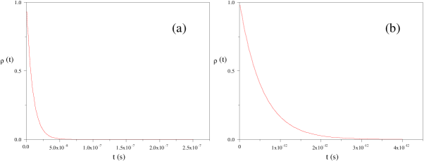
Figure 2: Damping of the non-diagonal terms of the density operator for two different values of $\tau$. For both cases we used $\Delta E=4\;$eV.  (a) Slower damping for $\tau=6.26\times 10^{-24}\;$s; (b) faster damping for $\tau=\times 10^{-19}\;$s.  This Figure is taken from Ref.[73].

5.5 Further comments

It should be noticed that the time-evolution operator (69) preserves trace, obeys the semigroup law, and implies an irreversible evolution towards a stationary diagonal form. In other words, notwithstanding the simplicity of the present “discrete” theory, that is, of the chronon approach, an intrinsic relation is present between measurement process and irreversibility: Indeed, the operator (13), meeting the properties of a semigroup, does not possess in general an inverse (and non-invertible operators are, of course, related to irreversible processes). For instance, in a measurement process in which the microscopic object is lost after the detection, one is just dealing with an irreversible process that could be well described by an operator like (69).

In our (discrete and retarded) theory, the “reduction” to the diagonal form

$$\rho(t)\vspace{1.0cm}\stackrel{{\scriptstyle t\rightarrow 0}}{{\rightarrow}}\vspace{1.0cm}\sum_{n}\rho_{nn}(0)|n\rangle\langle n|$$

is not instantaneous, but depends —as we have already seen— on the characteristic value $\tau$. More precisely, the non diagonal terms tend exponentially to zero according to a factor which, to the first order, is given by

$$\exp{\left|{\frac{-\omega_{nm}^{2}\tau t}{2}}\right|}\ .$$ (75)

Thus, the reduction to the diagonal form occurs, provided that $\tau$ possesses a finite value, no matter how small, and provided that $\omega_{nm}\tau$, for every n,m, is not much smaller than $1$; where

$$\omega_{nm}=(E_{n}-E_{m})/\hbar$$

are the transition frequencies between the different energy eigenstates (the last condition being always satisfied, e.g., for non-bounded systems).

It is essential to notice that decoherence has been obtained above, without having recourse to any statistical approach, and in particular without assuming any “coarse graining” of time. The reduction to the diagonal form illustrated by us is a consequence of the discrete (retarded) Liouville–von Neumann equation only, once the inequality $\omega_{nm}\tau\ll 1$ is not verified.

Moreover, the measurement problem is still controversial even with regard to its mathematical approach: In the simplified formalization introduced above, however, we have not included any consideration beyond those common to the quantum formalism, allowing an as clear as possible recognition of the effects of the introduction of a chronon.  Of course, we have not fully solved the quantum measurement problem, since clearly we have not yet found a model for determing which one of the diagonal values the actual experiment will reveal…

Let us however repeat that the introduction of a fundamental interval of time in approaching the measurement problem made possible a simple but effective formalization of the diagonal reduction process (through a mechanism that can be regarded as a decoherence caused by interaction with the environment [see Ref.[74] and refs. therein] only for the retarded case. This is not obtainable, whem taking into account the symmetric version of the discretized LvN equation.

It may be worthwhile to stress that the retarded form (68) of the direct discretization of the LvN equation is the same equation obtained via the coarse grained description (extensively adopted in [78, 79]).  This lead us to consider such an equation as a basic equation for describing complex systems, which is always the case when a measurement process is involved.

Let us add some brief remarks. First: the “decoherence” does not occur when we use the time evolution operators obtained directly from the retarded Schroedinger equation; the dissipative character of that equation, in fact, causes the norm of the state vector to decay with time, leading again to a non-unitary evolution operator: However, this operator (after having defined the density matrix) yields damping terms which act also on the diagonal terms! We discussed this point, as well a the question of the compatibility between Schroedinger’s picture and the formalism of the density matrix, have been analyzed by us in an Appendix of Ref.[73].  Second: the new discrete formalism allows not only the description of the stationary states, but also a (space-time) description of transient states: The retarded formulation yields a natural quantum theory for dissipative systems; and it is not without meaning that it leads to a simple explication of the diagonal reduction process.  Third: Since the composite system ${\cal O}\;+\;{\cal A}$ is a complex system, it is suitably described by the coarse grained description (exploited by Bonifacio in some important papers of his[78, 79]): it would be quite useful to increase our understanding of the relationship between the two mentioned pictures in order to get a deeper insight on the decoherence processes involved.

A further comment is the following. We have seen that the chronon formalism[73] has obvious connections with our views connection with our view about time, and space-time. But let us remind that the discrete formalism bears a further element of interest, since it possesses a non-hermitian character [as better clarified e.g. in the Appendices of Ref.[73]]. We know by now, for instance, that in the Schrödinger representation of such formalism, proper continuous equations can reproduce the outputs obtained with the discretized equations, once we replace the (discrete) conventional Hamiltonian by the suitable (continuous) equivalent, non-hermitian Hamiltonian. Indeed, one can find out a new Hamiltonian $\tilde{H}$ such that the new continuous Schrödinger equation

$$i\hbar{{\partial\Psi\left({\bf x,t}\right)}\over{\partial t}}=\tilde{H}\Psi\left({\bf x,t}\right)$$

reproduces, at the points $t=n\tau$, the same results obtained from the discretized equations.  Let us recall that Casagrande and Montaldi[82] showed it to be always possible to find out a continuous generating function that allows obtaining a differential equation equivalent to the original finite-difference one, such that at every point of interest their solutions are identical. This procedure, as we know, is useful also because it is ofter rather difficult to work with the finite–difference equations on a quantitative (and qualitative) basis. This equivalent Hamiltonian $\tilde{H}$ is non-hermitian; even if, as expected,  $\tilde{H}\rightarrow\hat{H}$  when  $\tau\rightarrow 0$.

Let us finally recall that, as previously mentioned, the chronon can have consequences in several different areas of physics: for instance, in Ref.[114] we derived spin was derived within a discrete-time approach.  As a further example, in the next subsection we want to report, with some details, on the possible role of the chronon in Cosmology.

5.6 On the chronon in Quantum Cosmology

As we were saying, the chronon can play a role also in recent theories referring, e.g., to the “archaic” universe: Theories which are group-theoretical approaches to quantum cosmology based on works by L.Fantappié and G.Arcidiacono. Those classical, interesting (and often forgotten) publications by Fantappié and by Arcidiacono form such a large theoretical background, that here, as far as it is concerned, we can only refer the readers to papers like the ones quoted in this subsection, as well as to Ref.[115] and refs. therein.

Let us here recall that, in terms of the Penrose terminology, the structure of quantum mechanics (QM) can be regarded as represented essentially by a unitary evolution operator $U$, acting upon on the wavefunction $\Psi$, and by the $\Psi$-collapse that we indicate by $R$. Some of the problems of QM are known to come out from the difficulty in connecting, loosely speaking, $U$ and $R$; indeed the collapse does not seem to be derivable from $U$.  A possible way out for conciliating $U$ and $R$ is by the introduction of the “pilot wave”, which leads however to problems with the meaning of $\Psi$. A view on QM which can help is the new Transactional Interpretation of QM [116, 117, 118].

Its first version, due to Cramer[119], regarded the non-local connections as a link between advanced and retarded potentials a la Wheeler-Feynman: But this arouse of course a lot of mathematical and conceptual problems, connected also to its too classical context. Intuitively the idea was rather simple: each particle “responded” to all its future possibilities… In the new version of the so-called Transactional Interpretation one does not meet any longer complication of this kind; and one just needs some simple rules about the opening and closing of the “transactions” in order to be able to fix in a univocal way the evolution operators.

Actually, at a fundamental level only the transactions between the field-modes take place, and the wave-function manifests itself as a statistical coverage of a large amount of elementary transitions.

In this context, the adoption of the chronon as a minimum duration of the transaction opening/ending is a possibly useful hypothesis, justified for instance by the role —as in Caldirola’s papers– of the classical electron radius, and the very range of strong interactions in particle physics; even if future developments in quantum gravity might shift the chronon value towards the Planck scale[120]… According to these views, physical processes whose duration is not larger than a chronon are possible only as virtual processes; so that cosmology could result to be connected with the foundations of QM.  Indeed, when the age of the “cosmos” (or rather of its precursor) did not exceed a chronon, it may be expected that all matter was associated with quantum virtual processes. By contrast, when the age of such a “cosmos” exceeded a chronon, the transactionals processes became possible and conversion of matter from the virtual to the real state could have taken place: This conversion might be nothing but what we call “big bang”.

Such an idea plays an important role in the theories of the Archaic Universe, when one refers indeed to a quantum vacuum still populated solely by virtual processes (without ordinary particles); and gets, among the others, that the geometry of such a vacuum becomes then a de Sitter Euclidean 5-dimensional (hyper)spherical surface. More specifically, the “archaic universe” theories go back to the group theoretical approaches proposed in the mentioned, classical works of Arcidiacono and Fantappié [121-126] wherein the Projective Relativity” was introduced.

Let us recall some basic concepts. Projective Relativity differs from the usual einsteinian Relativity in the existence of a de Sitter horizon, located at the same chronological distance from any observer. Because this distance does not depend on cosmic time, it is now the same as it was at the big bang time. But the existence of the a Sitter horizon in the past of an observer who emerged out from the big bang does imply in its turn the pre-existence of some form of spacetime, even before the big bang. In other words, before big-bang the aforementioned conversion process had to take place. In the meantime, no real matter existed; as a consequence, the geometry of this “pre-spacetime” must be that of the de Sitter space (according to the gravitational equations of Projective Relativity itself in the absence of matter). The inexistence of real processes could be seen, if you prefere, as the inexistence of time… It is terefore possible to assume that such an archaic universe was the four-dimensional surface of a five-dimensional hemisphere (cf. also Ref.[115] and refs. therein), that is, the Wick-rotated version of the de Sitter space. The “precursor” of time was, then, the five-dimensional distance from the plane of the equator; and the big bang happened when this time became equal to a chronon. Afterward, matter became real and real physical processes were started, requiring a radical change of geometry.

The new geometry will be connected to the “archaic” geometry via a Wick rotation (with the emergence of time); why the gravitational equations in presence of matter involved a scale reduction.  Using the Milne terminology, the public archaic spacetime now breaks down into a multitude of single private spacetimes (one for each “fundamental observer”), connected at the beginning by the de Sitter group. It may be even shown that this nucleation from the pre-vacuum can naturally recover, as a consequence of the geometry one had to adopt, the Hartle-Hawking condition[127].

6 Some conclusions

1. We have shown that the Time operator (1), hermitian even if non-selfadjoint, works for any quantum collisions or motions, in the case of a continuum energy spectrum, in non-relativistic quantum mechanics and in one-dimensional quantum electrodynamics. The uniqueness of the (maximal) hermitian time operator (1) directly follows from the uniqueness of the Fourier-transformations from the time to the energy representation. The time operator (1) has been fruitfully used in the case, for instance, of tunnelling times (see Refs.[24-28]), and of nuclear reactions and decays (see Refs.[10-13] and also Ref.[110]). We have discussed the advantages of such an approach with respect to POVM’s, which is not applicable for three-dimensional particle collisions, within a wide class of Hamiltonians.

The mathematical properties of the present Time operator have actually demonstrated — without introducing any new physical postulates — that time can be regarded as a quantum-mechanical observable, at the same degree of other physical quantities (spatial coordinates, energy, momentum,…).

The commutation relations (Eqs. (8), (22), (31)) here analyzed, and the uncertainty relations (9), result to be analogous to those known for other pairs of canonically conjugate observables (as for coordinate $\hat{x}$ and momentum $\hat{p}_{x}$, in the case of Eq.(9)). Of course, our new relations do not replace, but merely extend the meaning of the classic time and energy uncertainties, given e.g. in Ref.[41]. In subsection 2.6, we have studied the properties of Time, as an observable, for quantum-mechanical systems with discrete energy spectra.

2. Let us stress that the Time operator (1), and relations (2), (3), (4), (15), (16), have been used for the temporal analysis of nuclear reactions and decays in Refs.[10-13]; as well as of new phenomena, about time delays-advances in nuclear physics and about time resonances or explosions of highly excited compound nuclei, in Refs.[111-113,110]. Let us also recall that, besides the time operator, other quantities, to which (maximal) hermitian operators correspond, can be analogously regarded as quantum-physical observables: For example, von Neumann himself [8, 9, 45]) considered the case of the momentum operator $-i\partial/\partial x$ in a semi-space with a rigid wall orthogonal to the $x$-axis at $x=0$, or of the radial momentum $-i\partial/\partial r$, even if both act on packets defined only over the positive $x$ or $r$ axis, respectively.

Subsection 2.5 has been devoted to a new “hamiltonian approach”: namely, to the introduction of the analogue of the “Hamiltonian” for the case of the Time operator.

3. In Section 3, we have proposed a suitable generalization for the Time operator (or, rather, for a Space-Time operator) in relativistic quantum mechanics. For instance, for the Klein-Gordon case, we have shown that the hermitian part of the three-position operator $\hat{x}$ is nothing but the Newton-Wigner operator, and corresponds to a point-like position; while its anti-hermitian part can be regarded as yielding the sizes of an extended-type (ellipsoidal) localization. When dealing with a 4-position operator, one finds that the Time operator is selfadjoint for unbounded energy spectra, while it is a (maximal) hermitian operator when the kinetic energy, and the total energy, are bounded from below, as for a free particle. We have extensively made recourse, in the latter case, to bilinear forms, which dispense with the necessity of eliminating the lower point — corresponding to zero velocity — of the spectra. It would be interesting to proceed to further generalizations of the 3- and 4-position operator for other relativistic cases, and analyze the localization problems associated with Dirac particles, or in 2D and 3D quantum electrodynamics, etc. Work is in progress on time analyses in 2D quantum electrodynamic, for application, e.g., to frustrated (almost total) internal reflections. Further work has still to be done also about the joint consideration of particles and antiparticles.

4. Non-hermitian Hamiltonians can play an important role in the description of Unstable States, by associating the decaying “resonances” with the eigenvectors of quasi-hermitian Hamiltonians: But on this point we just referred the interested reader to Refs.[59, 40, 110].  In Sections 4 and 5 of this work we paid attention, instead, to the possible role non-hermitian Hamiltonians, and non-unitary time-evolution operators, the cases of the nuclear optical model, of microscopic quantum dissipation, and particularly with an approach to the measurement problem in QM in terms of the chronon.  We have particularly devoted Sect.5 to the chronon formalism —where the chronon is a “quantum” of time, in the sense specified above— for its obvious connection with our view of time, and of space-time; and also because that discrete formalism has a non-hermitian character[73].  As to quantum dissipation[68-93], we discussed e.g. a particular approach for getting decoherence through interaction with the environment[73, 74].  In Sect.4 we had however touched also questions related with collisions in absorbing media; mentioning the case of the optical model in nuclear physics. Without forgetting that non-hermitian operators show up even in the case of tunnelling — e.g., in fission phenomena — with quantum dissipation, and of quantum friction.  As we were saying, among the many approaches to quantum irreversibility, in Sec.4.3 we already anticipated the possible way, for obtaining a “reduction to diagonal form”, by the introduction of finite-difference equations (in terms of the “chronon”): And we have subsequently exploited at lenght this issue, for showing the consequences of the introduction of a chronon in classical physics and in quantum mechanics (Sect.5).

5. Let us eventually observe that the “dual equations” (26) and (27) seem to be promising also for the study the initial stage of our cosmos, when tunnellings can take place through the barriers which appear in quantum gravity in the limiting case of quasi-Schröedinger equations[128].

7 Acknowledgements

This paper is largely based on work developed by one of us (ER), along the years, in collaboration with V.S.Olkhovsky, and, in smaller parts, with P.Smrz, with R.H.A.Farias, and with S.P.Maydanyuk; while another of us (IL) achnowledges the collaboration of L.Chiatti.  Thanks are moreover due, for stimulating discussions or kind collaboration, to Y.Aharonov, A.Agodi, M.Baldo, R.Bonifacio, E.O.Capelas, H.E.Hernández-Figueroa, A.S.Holevo, V.L.Lyuboshitz, C.Meroni, R.Mignani, S.Paleari, A.Pennisi, V.Petrillo, U.V.G.Recami, P.Riva, G.Salesi, A.Santambrogio, and B.N.Zakhariev.  One of the authors’ home-page is  www.unibg.it/recami .

References

- [1] Pauli W 1926 Handbuch der Physik vol. 5/1 (Berlin: Ed. by S. Fluegge) p. 60
- [2] Pauli W 1980 General Principles of Quantum Theory (Berlin: Springer)
- [3] Olkhovsky V S and Recami E 1968 Nuovo Cimento A53 610
- [4] Olkhovsky V S and Recami E 1969 Nuovo Cimento A63 814
- [5] Olkhovsky V S and Recami E 1970 Lett. Nuovo Cim. (First Series) 4 1165
- [6] Olkhovsky V S 1973 Ukrainskiy Fiz. Zhurnal [in Ukrainian and Russian] 18 1910
- [7] Olkhovsky V S, Recami E and Gerasimchuk A 1974 Nuovo Cimento A22 263
- [8] Recami E An operator for the observable time 1976 in Recent Developments in Relativistic Q.F.T. and Its Application (Proc. of the XIII Karpatz Winter School on Theor. Phys.), vol.II, ed. by W.Karwowski (Wroclaw Univ.Press; Wroclaw), pp.251-265
- [9] Recami E A time operator and the time-energy uncertainty relation 1977 in The Uncertainty Principle and Foundation of Quantum Mechanics, ed. by C.Price and S.Chissik (J.Wiley; London), Chap.4, pp.21-28
- [10] Olkhovsky V S 1984 Sov. J. Part. Nucl. 15 130
- [11] Olkhovsky V S 1990 Nukleonika 35 99
- [12] Olkhovsky V S 1992 Atti Accademia Peloritana dei Pericolanti, Sci., Mat. e Nat. 70 21 and 135
- [13] Olkhovsky V S 1998 Mysteries, Puzzles and Paradoxes in Quantum Mechanics (ed. by R. Bonifaccio, AIP) pp.272-276
- [14] Holevo A S 1978 Rep. Math. Phys. 13 379
- [15] Holevo A S 1982 Probabilistic and Statistical Aspects of Quantum Theory (Amsterdam)
- [16] Srinivas M D and Vijayalakshmi R 1981 Pramana J. Phys. 16 173
- [17] Busch P, Grabowski M and Lahti P J 1994 Phys. Lett. A191 357
- [18] Kobe D H and Aguilera-Navarro V C 1994 Phys. Rev. A50 933
- [19] Blanchard P and Jadczyk A 1996 Helv. Phys. Acta 69 613
- [20] Grot N, Rovelli C and Tate R S 1996 Phys. Rev. A54 4676
- [21] Leo’n J 1997 J. Phys. A30 4791
- [22] Aharonov Y, Oppenhem J, Popescu S, Reznik B and Unruh W 1998 Phys. Rev. A57 4130
- [23] Atmanspacher H and Amann A 1998 Internat. J. Theor. Phys. 37 629
- [24] Olkhovsky V S and Recami E 1992 Phys. Rep. 214 339
- [25] Olkhovsky V S, Recami E, Raciti F and Zaichenko A K 1995 J. de Phys. (France) I 5 1351
- [26] Olkhovsky V S, Recami E and Jakiel J 2004 Phys. Rep. 398 133
- [27] Olkhovsky V S and Recami E 2007 Intern. J. Mod. Phys A22 5063
- [28] Olkhovsky V S and Agresti A 1997 Proc. of the Adriatico Research. Conf. on Tunneling and its Implications (World Sci.) pp.327–355
- [29] Giannitrapani R 1997 Int. J. Theor. Phys. 36 1575
- [30] Kijowski J 1999 Phys. Rev. A59 897
- [31] Toller M 1999 Phys. Rev. A59 960
- [32] Delgado V 1999 Phys. Rev. A59 1010
- [33] Muga J, Palao J and Leavens C 1999 Phys. Lett. A253 21
- [34] Egusquiza I L and Muga J G 1999 Phys. Rev. A61 012104
- [35] Kocha’nski P and Wo’dkievicz K 1999 Phys. Rev. A60 2689
- [36] Góźdź A and Dȩbicki M 2007 Phys. At. Nuclei 70 529
- [37] Zhi-Yong Wang and Cai-Dong Xiong 2007 Annals of Physics 322 2304
- [38] Recami E., Olkhovsky V.S. and Maydanyuk S.P. 2010 Int. J. Mod. Phys. A25 1785-1818
- [39] Naimark M A 1940 Izvestiya Akademii Nauk SSSR, seriya matematicheskaya [in Russian, partially in English] 1940 4 277
- [40] Recami E, Rodrigues W A and Smrz P 1983 Hadronic Journal 6 1773-1789
- [41] Olkhovsky V S and Recami E 2008 Int. J. Mod. Phys. B22 1877
- [42] Stone M H 1930 Proc. Nat. Acad. Sci. USA 16, issue no. 1
- [43] Akhiezer N I and Glazman I M 1981 The Theory of Linear Operators in Hilbert Space (Pitman; Boston, Mass.)
- [44] D ter Haar 1971 Elements of Hamiltonian Mechanics (Oxford)
- [45] Von Neumann J 1955 Mathematical foundations of quantum mechanics (Princeton Univ. Press, Princeton, N.J.)
- [46] Aharonov Y and Bohm D 1961 Phys. Rev. A122 1649
- [47] Naimark M A 1943 Izvestiya Akademii Nauk SSSR, seriya Matematika 7 237–244
- [48] Carleman T 1923 Sur les Equations Integrales Anoyau R el et Sym trique (Uppsala)
- [49] Schweber S 1961 An Introduction to Relativistic Quantum Field Theory Chapt.5.3 (Row, Peterson and Co.)
- [50] Akhiezer A I and Berestezky V B 1959 Quantum Electrodynamics [in Russian] (Fizmatgiz; Moscow)
- [51] Rosenbaum D M 1969 J. Math. Phys. 10 1127
- [52] Ka’lnay A J 1966 Boletin del IMAF (Co’rdoba) 2 11
- [53] Ka’lnay A J and Toledo B P 1967 Nuovo Cimento A48 997
- [54] Gallardo J A, Ka’lnay A J, Stec B A and Toledo B P 1967 Nuovo Cimento A48 1008
- [55] Gallardo J A, Ka’lnay A J, Stec B A and Toledo B P 1967 Nuovo Cimento A49 393
- [56] Gallardo J A, Ka’lnay A J and Risenberg S H 1967 Phys. Rev. 158 1484
- [57] Baldo M and Recami E 1969 Lett. Nuovo Cim. 2 613
- [58] Recami E 1970 Atti Accad. Naz. Lincei (Roma) 49 77
- [59] Agodi A, Baldo M and Recami E 1973 Annals of Physics 77 157
- [60] Feshbach H, Porter C E and Weisskopf V F 1954 Phys. Rev. 96 448
- [61] Hodgson P I 1963 The Optical Model of Elasstic Scattering (Clarendon Press; Oxford, UK)
- [62] Moldauer P A 1963 Nucl. Phys. 47 65
- [63] Koning A G, Delaroche J P 2003 Nucl. Phys. A713 231
- [64] Kunieda S, Chiba S, Shilata K, Ichihara A and Suchovitski E Sh 2007 J. Nucl. Sc. and Techn. 44 838
- [65] Nikolaiev M V and Olkhovsky V S 1977 Theor. Mathem. Phys. 31 418
- [66] Olkhovsky V S 1975 Theor. Mathem. Phys. 20 774
- [67] Olkhovsky V S and Zaichenko A K 1981 Nuovo Cimento A63 155
- [68] Caldirola P, Casati G and Prosperetti A 1978 Nuovo Cimento A43, 127
- [69] Caldirola P 1979 Rivista N. Cim. 2, issue no. 13
- [70] Caldirola P and Lugiato L 1982 Physica A116, 248
- [71] Caldirola P “Dissipation in quantum theory (40 years of research)”, 1983 Hadronic Journal 6, 1400-1433
- [72] Caldirola P and Montaldi E 1979 Nuovo Cimento B53 291
- [73] Farias A R H and Recami E “Introduction of a quantum of time (‘chronon’) and its consequences for the electron in quantum and classical physics”, 2010 Advances in Imaging & Electron Physics (AIEP) 163, 33-115 [83 printed pages].
- [74] Recami E and Farias A R H “A simple quantum (finite-difference) equation for dissipation and decoherence”, 2009 Nuovo Cimento B124, 765-776, and refs. therein
- [75] See, e.g., Dirac P.A.M. “The classical theory of electron” 1938 Proc. Royal Soc. A167 148
- [76] Caldirola P. 1956 Suppl. Nuovo Cim. 3 297; and 1979 Rivista Nuovo Cim. 2, issue no.13, and refs. therein. Cf. also Yaghjian A.D. 1992 Relativistic Dynamics of a Charged Sphere (Springer; Berlin)
- [77] Cf., e.g., Recami E. and Salesi G. 1998 Physical Review A57 98, and refs. therein
- [78] Bonifacio R 1983 Lett. N. Cim. 37 481
- [79] Bonifacio R. 1999 Nuovo Cimento B114 473
- [80] Bonifacio R and Caldirola P 1983 Lett. N. Cim. 38 615
- [81] Ghirardi G C and Weber T 1984 Lett. N. Cim. 39 157
- [82] Casagrande F and Montaldi E 1977 Nuovo Cimento A40 369
- [83] Mignani R 1983 Lett. N. Cim. 38 169
- [84] Caldirola P 1941 Nuovo Cimento 18 393
- [85] Janussis A, et al. Lett. N. Cim. 29 (1980) 259
- [86] Janussis A, et al. Lett. N. Cim. 30 (1981) 289
- [87] Janussis A, et al. Lett. N. Cim. 31 (1981) 533
- [88] Janussis A, et al. Lett. N. Cim. 35 (1982) 485
- [89] Janussis A, et al. Nuovo Cimento B67 (1982) 161
- [90] Janussis A, et al. Lett. N. Cim. 34 (1982) 571
- [91] Janussis A, et al. Lett. N. Cim. 39 (1984) 75
- [92] Janussis A, Brodimas G and Mignani R 1991 J. Phys. A: Math. Gen. 24 L775
- [93] Janussis A, Leodaris A and Mignani R 1995 Phys. Lett. A197 187
- [94] Caldirola P 1941 Nuovo Cimento 18 393
- [95] Kanai E 1948 Progr. Theor. Phys. 3 440
- [96] Angelopoulon P, et al. 1995 Int. J. Mod. Phys. B9 2083
- [97] Caldeira A and Leggett A 1983 Annals of Physics 149 374
- [98] Olkhovsky V S, Recami E and Salesi G 2002 “Tunneling through two successive barriers and the Hartman (Superluminal) effect” Europhysics Letters 57 879-884 [e-print quant-ph/0002022]
- [99] Recami E 2004 “Superluminal tunneling through successive barriers. Does QM predict infinite group-velocities? ” Journal of Modern Optics 51 913-923
- [100] Olkhovsky V S, Recami E and Zaichenko A K 2005 “Resonant and non-resonant tunneling through a double barrier” Europhysics Letters 70 712-718 [e-print arXiv:quant-th/0410128]
- [101] Aharonov Y, Erez N and Resnik B 2002 Phys. Rev. A65 no. 052124
- [102] Raciti F and Salesi G 1994 J. Phys.-I (France) 4 1783
- [103] Nimtz G, Spieker H and Brodowsky M 1994 J. Phys.-I (France) 4 1379
- [104] Caldirola P Lett. N. Cim. 16 (1976) 151
- [105] Caldirola P Lett. N. Cim. 17 (1976) 461
- [106] Caldirola P Lett. N. Cim. 18 (1977) 465
- [107] Mignani R 1983 Lett. N. Cim. 38 169
- [108] Santilli R M 1979 Hadronic Journal 2 1460
- [109] Santilli R M 1983 Foundations of Theoretical Mechanics, Vol.II: Birkhoffian Generalization of Hamiltonian Mechanics (Springer; Berlin)
- [110] Olkhovsky V S, Dolinska M E and Omelchenko S A 2006 Central European Journal of Physics 4(2) 1-18
- [111] Olkhovsky V S, Doroshko N L 1992 Europhys. Lett. 18(6) 483-486
- [112] D’Arrigo A, Doroshko N L, Eremin N V, Olkhovsky V S, et al. 1992 Nucl. Phys. A549 375-386
- [113] D’Arrigo A, Doroshko N L, Eremin N V, Olkhovsky V S, et al. 1993 Nucl. Phys. A564 217-226
- [114] Recami E and Salesi G “Deriving Spin within a Discrete-Time Theory” 2007 Foundations of Physics 37 277-294
- [115] Recami E “Relativity and Beyond”, Chap.16 in Albert Einstein, 1879-1979: Relativity, Cosmology and Quanta, ed. by F.de Finis and M.Pantaleo 1979 (Johnson Rep. Co., New York, N.Y.), Vol.2, pp.537-597; “Teoriya Otnositelnosti i ee Obobstchenya”, in Astrofizika, Kyanti i Teoriya Otnositelnosti, ed. by F.I.Fedorov (Mir, Moscow, 1982), Chap.4, pp.53-128; both being translations, into English and Russian respectively, of E.Recami, “Alcune Possibili Estensioni della Relatività”, Chapt18 in Astrofisica e Cosmologia, Gravitazione, Quanti e Relatività – Centenario di Einstein, ed. by M.Pantaleo 1979 (Giunti-Barbera, Florence), pp.1021-1097
- [116] Chiatti L 2012 arXiv: 1204.6636
- [117] Licata I 2013 Europ. Phys J. - Web of Conferences (in press).
- [118] Kastner R E 2013 The Transactional Interpretation of Quantum Mechanics (Cambridge Univ. Press, UK).
- [119] Cramer J G 1988 Int. J. Theor. Phys. 27 227-236
- [120] Licata I 1991 Hadronic J. 14 225-250
- [121] Fantappié L 1959 Collectanea Mathematica 11(2) 78-136
- [122] Arcidiacono G 1976 Gen. Rel. Grav. 7 885
- [123] Arcidiacono G 1977 Gen. Rel. Grav. 7 865
- [124] Licata I 2006 EJTP 3(10) 211-224
- [125] Licata I and Chiatti L 2009 Int. J. Theor. Phys. 48 1003 1018
- [126] Licata I and Chiatti L 2010 Int. J. Theor. Phys. 49 2379 2402
- [127] Hartle J and Hawking S 1983 Physical Review D28 2960
- [128] Olkhovsky V S, Maydanuyk S P, Del Popolo A. and Recami E “A Fully quantum model of Big-Bang”, 2012 in Theoretical Concepts in Quantum Mechanics (Intech), p.341-382: [ISBN 978-953-51-0088-1]; DOI 10.5772/2075.