Sensitivity to perturbations and quantum phase transitions

Abstract

The local density of states or its Fourier transform, usually called fidelity amplitude, are important measures of quantum irreversibility due to imperfect evolution. In this letter we study both quantities in a paradigmatic many body system: the Dicke Hamiltonian, where a single-mode bosonic field interacts with an ensemble of $N$ two-level atoms. This model exhibits a quantum phase transition in the thermodynamic limit while for finite instances the system undergoes a transition from quasi-integrability to quantum chaotic. We show that the width of the local density of states clearly points out the imprints of the transition from integrability to chaos but no trace remains of the quantum phase transition. The connection with the decay of the fidelity amplitude is also established.

The sensitivity to perturbations is one of the major impediments to fully control quantum systems. With the advent of quantum information and its technological development, which enable the manipulation of many body systems such as cold atoms in optical lattices Bloch , a deep understanding of the sources that perturb and deteriorate quantum evolutions is required qinfo ; casati . This would help us to develop strategies to protect and manipulate quantum systems, but also by analysing the response to perturbations one would be able to extract information from the actual dynamics.

In quantum evolutions, the effects of perturbations can be analyzed by measuring how difficult is to reverse a given dynamics, as it was proposed by Peres peres . To this end several figures of merit have been defined. Among them, the so-called local density of states (LDOS) or strength function, defined by Wigner wigner to describe the statistical behavior of perturbed eigenfunctions, has been extensively studied due to its connections with fundamental problems such as irreversibility, thermalization or dissipation in quantum systems rigol ; santos . Moreover, the LDOS provides significant information in quantum quenches, one of the simplest nonequilibrium quantum phenomena silva . Consider a one parameter dependent Hamiltonian $H(\lambda)$, with eigenenergies $E_{j}(\lambda)$ and eigenstates $|j(\lambda)\rangle$. The LDOS of an eigenstate $|i(\lambda_{0})\rangle$, that we call unperturbed, is defined as

$$\rho_{i}(E,\delta\lambda)=\sum_{j}|\left\langle j(\lambda)\mid i(\lambda_{0})\right\rangle|^{2}\delta(E-E_{ij}),$$ (1)

where $\delta\lambda=\lambda-\lambda_{0}$ and $E_{ij}=E_{j}(\lambda)-E_{i}(\lambda_{0})$. It is the distribution of the overlaps squared between the unperturbed and perturbed eigenstates. The LDOS has been studied in several systems with different perturbations wigner ; Flambaum ; Fyodorov ; Casati ; Cohen ; Wisniacki , and it is equivalent to the probability of work for a quantum quench silva . This quantity is also intimately related to other measures of irreversibility. In fact, the averaged LDOS is equal to the Fourier transform of the fidelity amplitude (FA),

$$O(t)=\mathrm{Tr}[U^{\dagger}_{\lambda_{0}+\delta\lambda}(t)U_{\lambda_{0}}(t)]$$ (2)

where $U_{\lambda_{0}}(t)$ is the evolution operator corresponding to the Hamiltonian $H(\lambda_{0})$, and $U_{\lambda_{0}+\delta\lambda}(t)$ corresponds the perturbed one that governs the backward evolution. Further, $O(t)$ is connected with other well-known quantity, the Loschmidt echo (LE), defined as $M_{\psi}(t)=|\langle\psi|U^{\dagger}_{\lambda_{0}+\delta\lambda}(t)U_{\lambda_{0}}(t)|\psi\rangle|^{2}$ for a given initial state $|\psi\rangle$. If we average the LE over initial states according to Haar measure (which is uniform over all quantum states in the Hilbert space) we obtain zanardi04 ; dankert :

$$\overline{M}(t)=\int d|\psi\rangle\,M_{\psi}(t)=\frac{[d+|O(t)|^{2}]}{d(d+1)},$$ (3)

where $d$ is the dimension of the Hilbert space. Thus, the width of the LDOS gives the characteristic time-scale for the decay of the FA and the averaged LE.

During the last years, a great deal of work has been devoted to characterize the sensitivity to perturbations and irreversibility using these three quantities, the LDOS, FA or LE prosen-rev ; jacquod ; scholarpedia . Several regimes were shown, and some of them appear to be universal jalabert ; diego . Despite the importance of correlated many body systems, not only from a theoretical point of view but also in actual experimental setups, most of these studies were focused in single body systems. Only a few recent contributions consider the LE and the FA for many body systems Izrailev ; zanardi ; zanardi2 ; zanardi3 ; OpSuscep ; manfredi1 ; manfredi2 ; Pastawski . In Ref. zanardi ; zanardi2 ; zanardi3 ; OpSuscep it is shown that the LE of the ground state is a good indicator of a quantum phase transition. These studies were carried out for a one-dimensional transverse Ising model and a Heisenberg spin chain by considering the ground state fidelity. Other works that consider the evolution of a many body system, approximated by self consistent hydrodynamical equations, found that the LE drops abruptly after a critical time manfredi1 ; manfredi2 . Despite the above evidence, little is known about the behaviour of the FA and the LDOS for general evolutions, where the excited region of the spectra of such many body systems is involved.

The goal of this letter is to study the LDOS and the FA in a paradigmatic many body system: the Dicke model, where a single bosonic field interacts with $N$ two-level atoms. This model exhibits a quantum phase transition in the thermodynamic limit ($N\rightarrow\infty$) when the parameter $\lambda$, that controls the strength of the interaction, crosses a critical value $\lambda_{c}$. On top of that, for finite $N$, the system undergoes a transition from quasi-integrability to quantum chaotic within the same region of parameters. Remarkably, an experimental realization of this model has been recently done using a superfluid gas in an optical cavity nature-dicke .

Here we show that the width $\Gamma$ of the LDOS, which provides the time-scale for the decay of the FA, has a well defined behaviour depending on which side of the transition belongs the unperturbed evolution. In the case where $\lambda_{0}<\lambda_{c}$, the width of the LDOS is a linear function of the strength of the perturbation $\delta\lambda$. However, if $\lambda_{0}>\lambda_{c}$, three regimes are observed. For sufficiently small $\delta\lambda$, so that first order perturbation theory is valid, the width grows linearly $\Gamma\sim\delta\lambda$. Then, a crossover to a Fermi golden rule regime in which $\Gamma\sim\delta\lambda^{2}$ is observed. Finally, for larger perturbations, $\Gamma$ grows linearly again. These results are consistent with those obtained in a banded random model initially studied by Wigner wigner ; Casati . In order determine whether the source of this behaviour is due to presence of the quantum phase transition, we also considered the Dicke model in the rotating wave approximation, where the Hamiltonian is quasi-integrable for every $\lambda$, but also displays a quantum phase transition. By comparing the results in these two situations, we were able to show that the transition in the behaviour of $\Gamma$ is related to the integrability-chaos transition and not to the quantum phase transition. Finally, we consider the decay of the FA, $O(t)$, and show the relation between the first two regimes of $\Gamma$ and the decay of $O(t)$.

We begin by describing the system that we consider: the single-mode Dicke Model. This model describes an ensemble of $N$ two-level atoms with level splitting $\omega_{0}$ coupled to a single bosonic mode of frequency $\omega$ via dipole interaction ($\hbar=1$):

$$H(\lambda)=\omega_{0}J_{z}+\omega\,a^{\dagger}a+\frac{\lambda}{\sqrt{2j}}(a^{\dagger}+a)(J_{+}+J_{-}),$$ (4)

in this case $J_{z}$ and $J_{\pm}$ are the collective angular momentum operators for a pseudospin of length $j=N/2$, $a$ and $a^{\dagger}$ are the bosonic operators of the field, and $\lambda$ is the atom-field coupling constant. In the thermodynamic limit, $N\rightarrow\infty$, this model exhibits a quantum phase transition at $\lambda_{c}=\sqrt{\omega\omega_{0}}/2$ where there is broken symmetry associated to the parity Hepp73 . When $\lambda<\lambda_{c}$ the system is in the normal phase, while for $\lambda>\lambda_{c}$ the system is in the superrandiant phase. For finite sized instances and sufficiently high $N$ it displays a crossover in its level statistics from Poissonian to a Wigner distribution at $\lambda\approx\lambda_{c}$ Brandes . We shall call this transition from quasi-integrable to quantum chaos. In this case the parity, $\Pi=\exp(i\pi\hat{N})$ with $\hat{N}=a^{\dagger}a+J_{z}+j$ the so-called excitation number, is a conserved quantity. Thus, the Hilbert space is split into two non-interacting subspaces with definite parity. On the other hand, if we neglect the counter rotating terms in the interaction, by applying the rotating wave approximation (RWA) Haroche , we can then define the following Hamiltonian:

$$H_{RWA}(\lambda)=\omega_{0}J_{z}+\omega a^{\dagger}a+{\frac{\lambda}{\sqrt{2j}}}(a^{\dagger}J_{-}+aJ_{+}),$$ (5)

that also exhibits a quantum phase transition in the thermodynamic limit, but it is quasi-integrable for every finite $N$ and $\lambda$ Brandes .

We will consider the system away from the thermodynamic limit. Since the parity is a conserved quantity, we have restricted to the odd subspace. The parameters that were used in our numerical simulations are such that the system is in scaled resonance, $\omega=\omega_{0}=1$, so that $\lambda_{c}=0.5$ and $\lambda_{c}^{RWA}=1$; $j=20$ corresponding to $N=40$; and we have truncated the bosonic mode to $n=350$. For the Hamiltonian of eq. (4) we have also checked that $N$ is high enough so that the level statistics obeys a Wigner distribution for $\lambda>\lambda_{c}$. Since we truncate the Hilbert space of the bosonic mode, we consider excited states whose energy does not change as the value of $n$ is increased. This was done in order to avoid numerical errors due to the truncation. In order to smooth fluctuations arising from individual wave functions, we compute the averaged LDOS: $\bar{\rho}(E,\delta\lambda)$. This is equivalent to consider a generalized LDOS for a microcanonical state located in a given energy window, $\frac{1}{N_{\Delta}}\sum_{j,|E-E_{j}|<\Delta}\left|j(\lambda_{0})\rangle\langle j(\lambda_{0})\right|$. The average was done using a window of 200 states around the eigenstate 500, similar results were obtained by averaging over other energy windows. In order to determine $\Gamma$ we have considered the distance from the mean value of the LDOS that contains 70$\%$ of the probability. That is, $\int^{\langle E\rangle+\sigma}_{\langle E\rangle-\sigma}\rho(E,\delta\lambda)dE=0.7\hskip 11.38092pt$ where $\langle E\rangle=\int E\;\rho(E,\delta k)dE$. Remarkably, the width of the averaged LDOS has another interesting interpretation as the fluctuations in the probability of work for a quantum quench starting from a microcanonical state in given energy window silva .

In Fig. 1 we display the width of the LDOS, $\Gamma$, as a function of the perturbation for some values of $\lambda_{0}$. There we can observe different behaviors depending on whether the Hamiltonian is quasi-integrable. On one hand, we can see a linear dependence with the perturbation for quasi-integrable systems, i.e. $H(\lambda_{0})$ (with small $\lambda_{0}$) and $H_{RWA}(\lambda_{0})$. On the other hand, for $H(\lambda_{0})$ and $\lambda_{0}>0.5$, we can identify three different regimes as a function of $\delta\lambda$. For small perturbations $\Gamma$ is a linear function of $\delta\lambda$, for moderate values of $\delta\lambda$ there is quadratic dependence, and finally for strong perturbations a linear dependence is achieved. The initial linear regime corresponds to the situation where first order perturbation holds. In this case, the matrix elements of the perturbation, defined as $H^{\prime}\equiv[H(\lambda_{0}+\delta\lambda)-H(\lambda_{0})]/\delta\lambda$, are such that $\frac{|H^{\prime}_{i,j}|\delta\lambda}{\Delta E}<1,$ where $\Delta E$ is the mean level spacing. In the inset of Fig. 1 we plot the value of the matrix elements of the perturbation in the basis of the unperturbed eigenstates. In the region of the spectra that we considered, $\Delta E\approx~{}0.07$ so that $\delta\lambda<0.003$. Thus, for $\delta\lambda>0.003$ a crossover from a linear to a quadratic regime is observed.

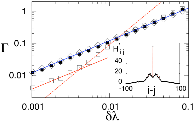
Figure 1: (Color online) Width of the LDOS as a function of the perturbation $\delta\lambda$ for: $\blacksquare$ $\lambda_{0}=0.1$; $\square$ $\lambda_{0}=0.8$; $\diamond$ $\lambda_{0}=1.6$ with the RWA. Inset: Mean value of the matrix elements $|H^{{}^{\prime}}_{i\;j}|$ as a function of $i-j$ for $\lambda_{0}=0.8$ in the unperturbed basis. See text for details.

As we will see, the appearance of a quadratic regime determines the range of perturbations where the LDOS has a Lorentzian shape [see Fig. 2 (b)]. Finally, for strong perturbations, a regime where $\Gamma$ depends linearly on $\delta\lambda$ is achieved, this is the non-perturbative regime. The last two regimes have been observed also in the banded random matrix model, as the one studied by Wigner wigner ; doron . Another conclusion that we can extract is that, if one considers moderate values of perturbations, the decay of the FA, given by the width of the LDOS, is faster for the quasi-integrable Hamiltonian than for the chaotic one. This is in agreement with the numerical simulations that are shown bellow [see Fig. 4].

Let us now consider the structure of the LDOS. In Fig. 2 we show the typical behavior of the mean LDOS for the Dicke model. If we consider $\lambda=0.8$ for $\delta\lambda<0.003$, as we discussed before, the LDOS is a Gaussian distribution [see Fig. 2 (a)]. This regime is characterized by the validity of the first order perturbation theory, so the overlap of unperturbed and perturbed states is approximately $\left\langle j(\lambda)\mid i(\lambda_{0})\right\rangle\sim\delta_{ij}$ and the gaussian distribution comes from the distributions of the eigenenergies that appear in Eq. 1. For greater values of $\delta\lambda$, first order perturbation theory is no longer valid and a crossover to a Lorentzian distribution is observed [see Fig. 2 (b)]. In Fig. 2 (c) and (d) we show the corresponding mean LDOS when $\lambda<\lambda_{c}$. In this case, the LDOS has no recognizable structure. Similar distributions were obtained for the RWA Hamiltonian.

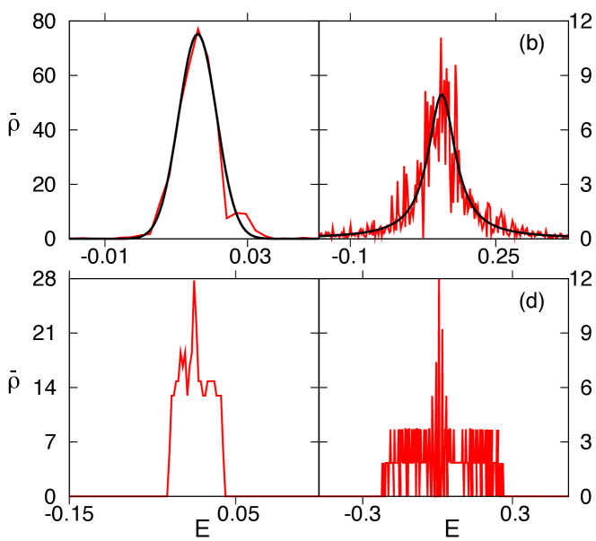
Figure 2: Mean LDOS $\bar{\rho}(E,\delta\lambda)$ for the Dicke model. The average was done using 200 states around the eigenstate with energy $E_{500}$. (a) $\delta\lambda=0.001$ and $\lambda_{0}=0.8$, (b) $\delta\lambda=0.08$ and $\lambda_{0}=0.8$, (c) $\delta\lambda=0.001$ and $\lambda_{0}=0.2$ and (d) $\delta\lambda=0.08$ and $\lambda_{0}=0.2$.

The transition from quasi-integrability to quantum chaos that appears in the Dicke Hamiltonian is reflected in the behavior of the width of the LDOS. This becomes evident when we compare the above results with the case where no such transition is present, the RWA Hamiltonian. In addition to this change in the spectral statistics, there is a quantum phase transition in the thermodynamic limit in both systems. However, Fig. 1 seems to indicate that no trace of this transition is present in the width of the LDOS for an excited region of the spectra. In order to show this in more detail, in Fig. 3 we plot the width of the LDOS in terms of $\lambda$ for a fixed small perturbation $\delta\lambda$. In Fig. 3 (a) we consider $\delta\lambda=0.001$, so we are in the regime where $\Gamma$ depends linearly with $\delta\lambda$ for the Dicke Hamiltonian and its RWA. In Fig. 3 (b) $\delta\lambda=0.06$, so $\Gamma$ depends quadratically with $\delta\lambda$ for the Dicke Hamiltonian. From the plot we can see that for small enough values of $\lambda$ this function is the same for both Hamiltonians, reflecting the fact that the RWA is a good approximation for small values of $\lambda$. As $\lambda$ is increased the value of $\Gamma$ decreases for the full Hamiltonian up to a value which is approximately $\lambda_{c}$ where it remains constant again. While when we consider the RWA Hamiltonian $\Gamma(\lambda)$ remains approximately constant for the full range. Therefore, $\Gamma(\lambda)$ behaves as an indicator of the quasi-integrable to quantum chaotic transition, but it does not show any trace of the quantum phase transition that is also present in the RWA. A related quantity that behaves in a similar way is the operator fidelity metric OpFidelity but, in contrast the width of the LDOS, it is time-dependent.

Figure 3: Width of the LDOS, $\Gamma$, as a function of $\lambda_{0}$ for a fixed small perturbation $\delta\lambda$. $\blacktriangle$ RWA, $\circ$ without RWA. In (a) $\delta\lambda=0.001$ and (b) $\delta\lambda=0.06$.

We turn now to the discussion of the behavior of the FA. In Fig. 4 we consider the modulus of the FA as a function of time. As in the previous results, the FA was computed by averaging 200 states around the eigenstate 500. We show some examples for the quasi-integrable region and for the quantum chaotic region. In Fig.4 (a) $\lambda=0.1$, so the system is quasi-integrable and in (b) we show the chaotic case using $\lambda=0.8$ Brandes . Comparing the decays for the same $\delta\lambda$ of Fig.4 (a) and (b) we can clearly see that if $\delta\lambda<0.01$ the quasi-integrable case decays faster than the chaotic one. If $\delta\lambda>0.01$ both cases decay approximately in the same way. As we said above, we could extract the same conclusion from looking at the width of the LDOS in Fig. 1, which provides a characteristic time-scale for the decay of the FA. Similar behavior was previously observed in one body systems prosen-rev . We would like to remark that, similarly to what happens in Pastawski , in this many body system no signatures of hypersensibility in which the FA or LE drops abruptly was observed manfredi1 ; manfredi2 .

We have also analyzed the short time decay of the modulus of the FA. When the system is quasi-integrable [Fig.4 (a)] and for $\delta\lambda<2\,10^{-2}$, the decay at short times is essentially Gaussian, and also displays some oscillations due to degeneracy. But, if the system is chaotic we can show that the time dependence of $|O(t,\delta\lambda)|$ is of the form,

$$|O(t,\delta\lambda)|\approx a\,e^{-b^{2}t^{2}}+(1-a)\,e^{-ct}.$$ (6)

for appropriate $a$, $b$ and $c$ that depend on $\lambda$ and $\delta\lambda$. For small perturbations is a linear combination of Gaussian and an exponential decay. As the perturbation is increased the value of $a$ tends to zero, and for the region where $\Gamma$ is quadratic with $\delta\lambda$ (see also Fig. 1) we recover the exponential decay.

Figure 4: Modulus of the FA $|O(t)|$ as a function of time. In (a) $\lambda=0.1$ and (b) $\lambda=0.8$, both without the RWA. The FA was computed using 200 states around the eigenstate with energy $E_{500}$. $\square$ $\delta\lambda=10^{-3}$, $\blacksquare$ $\delta\lambda=3.1\,10^{-3}$, $\circ$ $\delta\lambda=9.4\,10^{-3}$, $\bullet$ $\delta\lambda=2.9\,10^{-2}$, $\blacktriangle$ $\delta\lambda=8.7\,10^{-2}$.

Summarizing, we have considered the sensitivity to perturbations and the irreversible dynamics in the critical Dicke model by using the LDOS and the FA. We have studied the width of the LDOS, which defines the time-scale for the decay of the FA, and showed the appearance of three different regimes, depending on the strength of the perturbation, for the chaotic Hamiltonian. These regimes were also observed in a banded random matrix model defined by Wigner wigner ; Casati . On the other hand, for integrable Hamiltonians the width of the LDOS increases linearly with perturbation. We showed that the decay of the fidelity amplitude, given by the width of the LDOS $\Gamma(\lambda)$, is sensitive to the transition from quasi-integrability to quantum chaos. However, a proper comparison with its RWA shows that no trace of the phase transition can be found in the excited spectra. Thus, the FA is unable to detect the quantum phase transition unless the ground state fidelity is considered. Finally, we would also like to stress that our results have further applications in relation to the probability of work in quantum quenches.

- (1) I. Bloch, J. Dalibard and W. Zwerger Rev. Mod. Phys. 80, 885 (2008).
- (2) M. A. Nielsen and I. L. Chuang Quantum Computation and Quantum Information Cambridge, (2010).
- (3) G. Benenti, G. Casati and G. Strini, Principle of Quantum Computation and Information. Vol. II: Basic tools and special topics, World Scientific (2007).
- (4) A. Peres Phys. Rev. A, 30 1610 (1984).
- (5) E. P. Wigner, Ann. Math. 62, 548 (1955).
- (6) M. Rigol, V. Dunjko, and M. Olshanii, Nature (London) 452, 854 (2008).
- (7) L. F. Santos, F. Borgonovi and F. M. Izrailev, Phys. Rev. Lett. 108, 094102 (2012).
- (8) A. Silva, Phys. Rev. Lett. 101, 120603 (2008).
- (9) V. V. Flambaum, A. A. Gribakina, G. F. Gribakin, and M. G. Kozlov, Phys. Rev. A 50, 267 (1994).
- (10) Y. Fyodorov, O. Chubykalo, F. Izrailev, and G. Casati, Phys. Rev. Lett. 76, 1603 (1996).
- (11) G. Casati, B. V. Chirikov, I. Guarneri, and M. Izrailev, Phys. Lett. A 223, 430 (1996).
- (12) D. Cohen and E. J. Heller, Phys. Rev. Lett. 84, 2841 (2000).
- (13) D. A. Wisniacki, N. Ares and E. G. Vergini, Phys. Rev. Lett. 104, 254101 (2010).
- (14) P. Zanardi and D. A. Lidar, Phys. Rev. A 70, 012315 (2004).
- (15) Ch. Dankert, arXiv:quant-ph/0512217 (2005).
- (16) Ph. Jacquod and C. Petitjean, Adv. Phys. 58, 67 (2009).
- (17) A. Goussev, R. Jalabert, H. Pastawski and D. A. Wisniacki, Scholarpedia 7, 11687 (2012).
- (18) T. Gorin, T. Prosen, T. H. Seligman, M. Z̆nidaric̆, Phys. Rep. 435, 33 (2006).
- (19) R. A. Jalabert and H. M. Pastawski, Phys. Rev. Lett. 86, 2490 (2001).
- (20) D. A. Wisniacki, D. Cohen, Phys. Rev. E 66, 046209 (2002).
- (21) V. V. Flambaum, and F. M. Izrailev, Phys. Rev. E 64, 026124 (2001).
- (22) H. Quan, Z. Song, X. Liu, P. Zanardi, and C. Sun, Phys. Rev. Lett. 96, 140604 (2006).
- (23) P. Zanardi, and N. Paunković, Phys. Rev. E 74, 031123 (2006).
- (24) X. Lu, Z. Sun, X. Wang, and P. Zanardi, Phys. Rev. A 78, 032309 (2008).
- (25) X. Wang, Z. Sun, and Z. D. Wang, Phys. Rev. A 79, 012105 (2009).
- (26) G. Manfredi, P. A. Hervieux, Phys. Rev. Lett. 97, 190404 (2006).
- (27) G. Manfredi, P. A. Hervieux, Phys. Rev. Lett. 100, 050405 (2008).
- (28) P. R. Zangara, A. D. Dente, P. R. Levstein, and H. M. Pastawski, Phys. Rev. A 86, 012322 (2012)
- (29) K. Baumann, G. Guerlin, F. Brennecke, T. Esslinger, Nature 464, 140604 (2010).
- (30) K. Hepp and E. H. Lieb, Ann. Phys. (N.Y.) 76, 360 (1973).
- (31) C. Emary and T. Brandes, Phys. Rev. Lett. 90, 044101 (2003); C. Emary and T. Brandes, Phys. Rev. E 67, 066203 (2003).
- (32) S. Haroche and J.-M. Raimond, Exploring the Quantum, Atoms, Cavities and Photons, Oxford Univ. Press, (2006).
- (33) M. Hiller, D. Cohen, T. Geisel, T. Kottos Ann. of Phys. 321, 1025 (2006).
- (34) P. Giorda and P. Zanardi, Phys. Rev. E 81, 017203 (2010).