Numerical calculation of the runaway electron distribution function and associated synchrotron emission

Abstract

Synchrotron emission from runaway electrons may be used to diagnose plasma conditions during a tokamak disruption, but solving this inverse problem requires rapid simulation of the electron distribution function and associated synchrotron emission as a function of plasma parameters. Here we detail a framework for this forward calculation, beginning with an efficient numerical method for solving the Fokker-Planck equation in the presence of an electric field of arbitrary strength. The approach is continuum (Eulerian), and we employ a relativistic collision operator, valid for arbitrary energies. Both primary and secondary runaway electron generation are included. For cases in which primary generation dominates, a time-independent formulation of the problem is described, requiring only the solution of a single sparse linear system. In the limit of dominant secondary generation, we present the first numerical verification of an analytic model for the distribution function. The numerical electron distribution function in the presence of both primary and secondary generation is then used for calculating the synchrotron emission spectrum of the runaways. It is found that the average synchrotron spectra emitted from realistic distribution functions are not well approximated by the emission of a single electron at the maximum energy.

I Introduction

Due to the decrease in the Coulomb collision cross section with velocity, charged particles in an electric field can “run away” to high energies. In tokamaks, the resulting energetic particles can damage plasma-facing components and are expected to be a significant danger in the upcoming ITER experiment. Electrons are typically the species for which runaway is most significant Dreicer (1960); Connor and Hastie (1975), but runaway ions Furth and Rutherford (1972) and positrons Helander and Ward (2003); Fülöp and Papp (2012) can also be produced. Relatively large electric fields are required for runaway production, and in tokamaks these can arise during disruptions or in sawtooth events. Understanding of runaway electrons and their generation and mitigation is essential to planning future large experiments such as ITER.

Runaway electrons emit measurable synchrotron radiation, which can potentially be used to diagnose the distribution function, thereby constraining the physical parameters in the plasma. The runaway distribution function and associated synchrotron emission depend on the time histories of the local electric field $E$, temperature $T$, average ion charge $Z$, and density $n$. To infer these quantities (and the uncertainty in these quantities) inside a disrupting plasma using the synchrotron emission, it is necessary to run many simulations of the runaway process, scanning the various physical parameters. To make such a scan practical, computational efficiency is important.

To this end, in this work we demonstrate a framework for rapid computation of the runaway distribution function and associated synchrotron emission for given plasma parameters. The distribution function is computed using a new numerical tool named CODE (COllisional Distribution of Electrons). Physically, the distribution function is determined by a balance between acceleration in the electric field and collisions with both electrons and ions. The calculation in CODE is fully relativistic, using a collision operator valid for both low and high velocities Papp et al. (2011) and it includes both primary and secondary runaway electron generation. If primary runaway electron generation dominates, CODE can be used in both time-dependent and time-independent modes. The latter mode of operation, in which a long-time quasi-equilibrium distribution function is calculated, is extremely fast in that it is necessary only to solve a single sparse linear system. Due to its speed and simplicity, CODE is highly suitable for coupling within larger more expensive calculations. Besides the inverse problem of determining plasma parameters from synchrotron emission, other such applications could include the study of instabilities driven by the anisotropy of the electron distribution function, and comprehensive modeling of disruptions.

Other numerical methods for computing the distribution function of runaways have been demonstrated previously, using a range of algorithms. Particle methods follow the trajectories of individual marker electrons. Deterministic particle calculations Martín-Solís et al. (1998) can give insight into the system behavior but cannot calculate the distribution function, since diffusion is absent. Collisional diffusion may be included by making random adjustments to particles’ velocities, an approach which has been used in codes such as ASCOTHeikkinen et al. (1993) and ARENAEriksson and Helander (2003). For a given level of numerical uncertainty (noise or discretization error), we will demonstrate that CODE is more than 6 orders of magnitude faster than a particle code on the same computer. Other continuum codes developed to model energetic electrons include BANDITO’Brien et al. (1986), CQL3DChiu et al. (1998); Harvey et al. (2000) and LUKE Peysson et al. (2003); Peysson and Decker (2008). These sophisticated codes were originally developed to model RF heating and current drive, and contain many features not required for the calculations we consider. For example, CQL3D contains $\sim 90,000$ lines of code and LUKE contains $\sim 118,000$ lines, whereas CODE contains $<1,200$ lines (including comments). While future more elaborate modeling may require the additional features of a code like CQL3D or LUKE, for the applications we consider, we find it useful to have the nimble and dedicated tool CODE. For calculations of non-Maxwellian distribution functions in the context of RF heating, an adjoint method Karney and Fisch (1986) can be a useful technique for efficient solution of linear inhomogeneous kinetic equations. However, the kinetic equation we will consider is nonlinear (if avalanching is included) and homogeneous, so the adjoint method is not applicable.

In several previous studies, a single particle with a representative momentum and pitch-angle is used as an approximation for the entire runaway distribution Jaspers et al. (2001); Yu et al. (2013) when computing the synchrotron emission. In this paper, we present a computation of the synchrotron radiation spectrum of a runaway distribution in various cases. By showing the difference between these spectra and those based on single particle emission we demonstrate the importance of taking into account the entire distribution.

The remainder of the paper is organized as follows. In Sec. II we present the kinetic equation and the collision operator used. Section III details the discretization scheme and calculation of the primary runaway production rate, with typical results shown in section IV. The avalanche source term and its implementation are described in Sec. V. In this section we also demonstrate agreement with an analytic model for the distribution function Fülöp et al. (2006). Computation of the synchrotron emission spectrum from the distribution function is detailed in Sec. VI, and comparisons to single-particle emission are given. We conclude in Sec. VII.

II Kinetic Equation and Normalizations

We begin with the kinetic equation

$$\frac{\partial f}{\partial t}-eE\mbox{\boldmath$b$}\cdot\nabla_{\mbox{\boldmath$p$}}f=C\{f\}+S.$$ (1)

Here, $-e$ is the electron charge, $E$ is the component of the electric field along the magnetic field, $\mbox{\boldmath$b$}=\mbox{\boldmath$B$}/B$ is a unit vector along the magnetic field, $\nabla_{\mbox{\boldmath$p$}}$ is the gradient in the space of relativistic momentum $\mbox{\boldmath$p$}=\gamma m\mbox{\boldmath$v$}$, $\gamma=1/\sqrt{1-v^{2}/c^{2}}$, $v=|\mbox{\boldmath$v$}|$ is the speed, $m$ is the electron rest mass, $c$ is the speed of light, $C$ is the electron collision operator, and $S$ represents any sources. All quantities refer to electrons unless noted otherwise. Equation (1) is the large-aspect-ratio limit of the bounce- and gyro-averaged Fokker-Planck equation (e.q. (2) in (Rosenbluth and Putvinski (1997))). Particle trapping effects are neglected, which is reasonable since runaway beams are typically localized close to the magnetic axis. We may write $\mbox{\boldmath$b$}\cdot\nabla_{\mbox{\boldmath$p$}}f$ in (1) in terms of scalar variables using

$$\mbox{\boldmath$b$}\cdot\nabla_{\mbox{\boldmath$p$}}f=\xi\frac{\partial f}{\partial p}+\frac{1-\xi^{2}}{p}\frac{\partial f}{\partial\xi}$$ (2)

where $p=|\mbox{\boldmath$p$}|$, and $\xi=\mbox{\boldmath$p$}\cdot\mbox{\boldmath$b$}/p$ is the cosine of the pitch angle relative to the magnetic field. The distribution function is defined such that the density $n$ is given by $n=\int d^{3}p\;f$, so $f$ has dimensions of $(\mathrm{length}\times\mathrm{momentum})^{-3}$, and we assume the distribution function for small momentum to be approximately the Maxwellian $f_{\mathrm{M}}=n\pi^{-3/2}(mv_{\mathrm{e}})^{-3}\exp(-y^{2})$ where $v_{\mathrm{e}}=\sqrt{2T/m}$ is the thermal speed, and $y=p/(mv_{\mathrm{e}})=\gamma v/v_{\mathrm{e}}$ is the normalized momentum.

We use the collision operator from Appendix B of Ref. Papp et al. (2011). This operator is constructed to match the usual nonrelativistic test-particle operator in the limit of $v\ll c$, and in the relativistic limit it reduces to the operator from Appendix A of Ref. Sandquist et al. (2006). The collision operator is

$$C\{f\}=\frac{1}{p^{2}}\frac{\partial}{\partial p}p^{2}\left[C_{A}\frac{\partial f}{\partial p}+C_{F}f\right]+\frac{C_{B}}{p^{2}}\frac{\partial}{\partial\xi}(1-\xi^{2})\frac{\partial f}{\partial\xi}$$ (3)

where

$$C_{A} = \frac{\Gamma}{v}\Psi(x),$$ (4)

$$C_{B} = \frac{\Gamma}{2v}\left[Z+\phi(x)-\Psi(x)+\frac{\delta^{4}x^{2}}{2}\right],$$ (5)

$$C_{F} = \frac{\Gamma}{T}\Psi(x),$$ (6)

$\delta=v_{\mathrm{e}}/c$, $x=v/v_{\mathrm{e}}=y/\sqrt{1+\delta^{2}y^{2}}$, $Z$ is the effective ion charge,

$$\Gamma=4\pi ne^{4}\ln\Lambda=(3\sqrt{\pi}/4)\nu_{\mathrm{ee}}v_{\mathrm{e}}^{3}m^{2}$$ (7)

is identical to the $\Gamma$ defined in Refs. Papp et al. (2011); Sandquist et al. (2006); Karney and Fisch (1985), $\nu_{\mathrm{ee}}=4\sqrt{2\pi}e^{4}n\ln\Lambda/(3\sqrt{m}T^{3/2})$ is the usual Braginskii electron collision frequency, $\phi(x)=2\pi^{-1/2}\int_{0}^{x}\exp(-s^{2})\,ds$ is the error function, and

$$\Psi(x)=\frac{1}{2x^{2}}\left[\phi(x)-x\frac{d\phi}{dx}\right]$$ (8)

is the Chandrasekhar function. In the nonrelativistic limit $\delta\to 0$, then $y\to x$, and (3) reduces to the usual Fokker-Planck test-particle electron collision operator.

The collision operator (3) is approximate in several ways. First, it originates from the Fokker-Planck approximation in which small-angle collisions dominate, which is related to an expansion in $\ln\Lambda\gg 1$. Consequently, the infrequent collisions with large momentum exchange are ignored, so the secondary avalanche process is not included at this stage, but will be addressed later in Sec. V. Also, the modifications to the Rosenbluth potentials associated with the high-energy electrons are neglected, i.e. collisions with high-energy field particles are ignored.

The kinetic equation is normalized by multiplying through with $m^{3}v_{\mathrm{e}}^{3}\pi^{3/2}/(\nu_{\mathrm{ee}}n)$, and defining the normalized distribution function

$$F=(\pi^{3/2}m^{3}v_{\mathrm{e}}^{3}/n)f$$ (9)

so that $F\to 1$ at $p\to 0$. We also introduce a normalized electric field

$$\hat{E}=-eE/(mv_{\mathrm{e}}\nu_{\mathrm{ee}})$$ (10)

which, up to a factor of order unity, is $E$ normalized by the Dreicer field. The normalized time is $\hat{t}=\nu_{\mathrm{ee}}t$ and the normalized source is $\hat{S}=Sm^{3}v_{\mathrm{e}}^{3}\pi^{3/2}/(\nu_{\mathrm{ee}}n)$. We thereby obtain the dimensionless equation

$$\frac{\partial F}{\partial\hat{t}}+\hat{E}\xi\frac{\partial F}{\partial y}+\hat{E}\frac{1-\xi^{2}}{y}\frac{\partial F}{\partial y}-\frac{3\sqrt{\pi}}{4}\frac{1}{y^{2}}\frac{\partial}{\partial y}y^{2}\left[\frac{\Psi(x)}{x}\frac{\partial F}{\partial y}+2\Psi(x)F\right]$$ (11)

$$-\frac{3\sqrt{\pi}}{4}\frac{1}{2xy^{2}}\left[Z+\phi(x)-\Psi(x)+\frac{\delta^{4}x^{2}}{2}\right]\frac{\partial}{\partial\xi}(1-\xi^{2})\frac{\partial F}{\partial\xi} = \hat{S}.$$

Notice that this equation has the form of a linear inhomogeneous 3D partial differential equation:

$$\frac{\partial F}{\partial\hat{t}}+MF=\hat{S}$$ (12)

for a linear time-independent differential operator $M$. If a time-independent equilibrium solution exists, it will be given by $F=M^{-1}\hat{S}$.

Since both the electric field acceleration term and the collision operator in the kinetic equation (1) have the form of a divergence of a flux in velocity space, the total number of particles is constant in time in the absence of a source: $(d/dt)\int d^{3}p\;f=\int d^{3}p\;S$. However, runaway electrons are constantly gaining energy, so without a source at small $p$ and a sink at large $p$, no time-independent distribution function will exist. From another perspective, a nonzero source is necessary to find a nonzero equilibrium solution of (11), because when $\hat{S}=0$, (11) with $\partial/\partial\hat{t}=0$ is a homogeneous equation with homogeneous boundary conditions. (The boundary conditions are that $F$ be regular at $y=0$, $\xi=-1$, and $\xi=1$, and that $f\to 0$ as $y\to\infty$.) Thus, the solution of the time-independent problem $F=M^{-1}\hat{S}$ for $\hat{S}=0$ would be $F=0$.

To find a solution, we must either consider a time-dependent problem or include a nonzero $S$. In reality, spatial transport can give rise to both sources and sinks, and a sink exists at high energy due to radiation. When included, secondary runaway generation (considered in Sec. V) also introduces a source. To avoid the added complexity of these sinks and sources and simultaneously avoid the intricacies of time dependence, when restricting ourselves to primary generation we may formulate a time-independent problem as follows. We take $\hat{S}=\alpha e^{-y^{2}}$ for some constant $\alpha$, representing a thermal source of particles. Equation (11) for $\partial/\partial\hat{t}=0$ may be divided through by $\alpha$ and solved for the unknown $F/\alpha$. Then $\alpha$ may be determined by the requirement $F(p=0)=1$, and $F$ is then obtained by multiplying the solution $F/\alpha$ by this $\alpha$.

The constant $\alpha$ represents the rate at which particles must be replenished at low energy to balance their flux in velocity space to high energy. Therefore, $\alpha$ is the rate of runaway production. As we do not introduce a sink at high energies, $F$ will have a divergent integral over velocity space.

CODE can also be run in time-dependent mode. Once the velocity space coordinates and the operator $M$ are discretized, any implicit or explicit scheme for advancing a system of ordinary differential equations (forward or backward Euler, Runge-Kutta, trapezoid rule, etc.) may be applied to the time coordinate. (Results shown in this paper are computed using the trapezoid rule.) Due to the diffusive nature of $M$, numerical stability favors implicit time-advance schemes.

III Discretization

We first expand $F$ in Legendre polynomials $P_{L}(\xi)$:

$$F(y,\xi)=\sum_{L=0}^{\infty}F_{L}(y)P_{L}(\xi).$$ (13)

Then the operation

$$\frac{2L+1}{2}\int_{-1}^{1}P_{L}(\xi)(\;\;\;\cdot\;\;\;)d\xi$$ (14)

is applied to the kinetic equation. Using the identities in the appendix, we obtain

$$\frac{\partial F_{L}}{\partial\hat{t}}+\sum_{\ell=0}^{\infty}\left\{\hat{E}\left[\frac{L+1}{2L+3}\delta_{L+1,\ell}+\frac{L}{2L-1}\delta_{L-1,\ell}\right]\frac{\partial}{\partial y}\right.$$ (15)

$$+\frac{\hat{E}}{y}\left[\frac{(L+1)(L+2)}{2L+3}\delta_{L+1,\ell}-\frac{(L-1)L}{2L-1}\delta_{L-1,\ell}\right]$$

$$-\frac{3\sqrt{\pi}}{4}\frac{\Psi(x)}{x}\delta_{L,\ell}\frac{\partial^{2}}{\partial y^{2}}-\frac{3\sqrt{\pi}}{2}\left[\frac{2\Psi(x)}{y}+\frac{dx}{dy}\frac{d\Psi}{dx}\right]\delta_{L,\ell}$$

$$-\frac{3\sqrt{\pi}}{4}\left[\frac{1}{x}\frac{dx}{dy}\frac{d\Psi}{dx}+\frac{2\Psi(x)}{xy}-\frac{\Psi(x)}{x^{2}}\frac{dx}{dy}+2\Psi(x)\right]\delta_{L,\ell}\frac{\partial}{\partial y}$$

$$\left.+\frac{3\sqrt{\pi}}{8xy^{2}}\left[Z+\phi(x)-\Psi(x)+\frac{\delta^{4}x^{2}}{2}\right]L(L+1)\delta_{L,\ell}\right\}F_{\ell} = \hat{S}_{L}$$

where $dx/dy=(1+\delta^{2}y^{2})^{-3/2}$, $d\Psi/dx=2\pi^{-1/2}e^{-x^{2}}-(2/x)\Psi(x)$, and $\hat{S}_{L}=(2L+1)\,2^{-1}\int_{-1}^{1}\hat{S}\;d\xi$ is the appropriate Legendre mode of $\hat{S}(y,\xi)=\sum_{L=0}^{\infty}\hat{S}_{L}(y)P_{L}(\xi)$. Note that the collision operator is diagonal in the $L$ index, and the electric field acceleration term is tridiagonal in $L$.

It is useful to examine the $L=0$ case of (15), which corresponds to (half) the integral of the kinetic equation over $\xi$:

$$\frac{\partial F_{0}}{\partial\hat{t}}-\frac{1}{y^{2}}\frac{\partial}{\partial y}\left[-y^{2}\frac{\hat{E}}{3}F_{1}+\frac{3\sqrt{\pi}}{4}y^{2}\left\{\frac{\Psi(x)}{x}\frac{\partial F_{0}}{\partial y}+2\Psi(x)F_{0}\right\}\right]=\hat{S}_{0}.$$ (16)

Applying $4\pi^{-1/2}\int_{y_{b}}^{\infty}dy\;y^{2}(\;\;\;\cdot\;\;\;)$ for some boundary value $y_{b}$, and assuming the source is negligible in this region, we obtain

$$\frac{1}{\nu_{\mathrm{ee}}n}\frac{dn_{r}}{d\hat{t}}=-\frac{4}{\sqrt{\pi}}\left[-y^{2}\frac{\hat{E}}{3}F_{1}+\frac{3\sqrt{\pi}}{4}y^{2}\left\{\frac{\Psi(x)}{x}\frac{\partial F_{0}}{\partial y}+2\Psi(x)F_{0}\right\}\right]_{y=y_{b}}$$ (17)

where $n_{r}$ is the number of runaways, meaning the number of electrons with $y>y_{b}$, so that $n_{r}=\int_{y>y_{b}}d^{3}p\;f=2\pi\int_{mv_{\mathrm{e}}y_{b}}^{\infty}dp\;p^{2}\int_{-1}^{1}d\xi\;f$. The runaway rate calculated from (17) should be independent of $y_{b}$ in steady state (as long as $y_{b}$ is in a region of $\hat{S}_{0}=0$), which can be seen by applying $\int_{y_{b1}}^{y_{b2}}dy\;y^{2}(\;\;\;\cdot\;\;\;)$ to (16). We find in practice it is far better to compute the runaway production rate using (17) than from the source magnitude $\alpha$, since the latter is more sensitive to the various numerical resolution parameters.

To discretize the equation in $y$, we can apply fourth-order finite differences on a uniform grid. Alternatively, for greater numerical efficiency, a coordinate transformation can be applied so grid points are spaced further apart at high energies. The $y$ coordinate is cut off at some finite maximum value $y_{max}$. The appropriate boundary conditions at $y=0$ are $dF_{0}/dy=0$ and $F_{L}=0$ for $L>0$. For the boundary at large $y$, we impose $F_{L}=0$ for all $L$. This boundary condition creates some unphysical grid-scale oscillation at large $y$, which may be eliminated by adding an artificial diffusion $c_{1}y^{-2}(\partial/\partial y)y^{2}\exp(-[y-y_{max}]/c_{2})\partial/\partial y$ localized near $y_{max}$ to the linear operator. Suitable values for the constants are $c_{1}=0.01$ and $c_{2}=0.1$. This term effectively represents a sink for particles, which must be included in the time-independent approach due to the particle source at thermal energies. Since this diffusion term is exponentially small away from $y_{max}$, the distribution function is very insensitive to the details of the ad-hoc term except very near $y_{max}$. All results shown hereafter are very well converged with respect to doubling the domain size $y_{max}$, indicating the results are insensitive to the details of the diffusion term.

IV Results for primary runaway electron generation

Figure 1 shows typical results from a time-independent CODE computation. To verify convergence, we may double $N_{\xi}$ (the number of Legendre modes), double $N_{y}$ (the number of grid points in $y$), and double the maximum $y$ ($y_{max})$ at fixed $y$ grid resolution (which requires doubling $N_{y}$ again.) As shown by the overlap of the solid red and dashed blue curves in Fig. 1a, excellent convergence is achieved for the parameters used here. Increasing the ad-hoc diffusion magnitude $c_{1}$ by a factor of 10 for the parameters of the red curve causes a relative change in the runaway rate (computed using (17) for $y_{b}=10$) of $|dn_{r}/d\hat{t}(c_{1}=0.1)-dn_{r}/d\hat{t}(c_{1}=0.01)|/[dn_{r}/d\hat{t}(c_{1}=0.01)]<10^{-9}$, demonstrating the results are highly insensitive to this diffusion term. As expected, the distribution function is increased in the direction opposite to the electric field ($p_{||}>0$). While the distribution function is reduced in the direction parallel to the electric field ($p_{||}<0$) for $y<5$, $F$ is actually slightly increased for $y>5$ due to pitch-angle scattering of the high-energy tail electrons, an effect also seen in Fokker-Planck simulations of RF current drive Karney and Fisch (1979). The pitch-angle scattering term can be artificially suppressed in CODE, in which case $F$ is reduced in the direction parallel to the electric field for all $y$.

Figure 2 compares the distribution functions obtained from the time-independent and time-dependent approaches. At sufficiently long times, the time-dependent version produces results that are indistinguishable from the time-independent version.

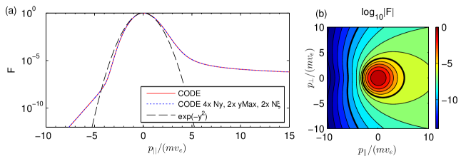
Figure 1: (Color online) Typical results of CODE, obtained for $\delta=0.1$, $\hat{E}=0.1$, and $Z=1$. (a) Normalized distribution function $F$ for $p_{\bot}=0$. Results are plotted for two different sets of numerical parameters ($\{N_{y}=300,y_{max}=20,N_{\xi}=20\}$ and $\{N_{y}=1200,y_{max}=40,N_{\xi}=40\}$). The results overlap completely, demonstrating excellent convergence. A Maxwellian is also plotted for comparison. (b) Contours of $F$ at values $10^{z}$ for integer $z$. Bold contours indicate $F=10^{-5}$ and $10^{-10}$.

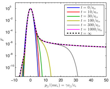
Figure 2: (Color online) The distribution function from time-dependent CODE at various times. At $t=1000/\nu_{\mathrm{ee}}$, the distribution function is indistinguishable from the solution obtained using the time-independent scheme ($t=\infty$) over the momentum range shown.

For comparison with previously published results, we show in Figure 3 results by Kulsrud et al Kulsrud et al. (1973), who considered only the nonrelativistic case $\delta\to 0$. The agreement with CODE is exceptional. The runaway production rate in CODE is computed using (17) for $y_{b}=10$. (Any value of $y_{b}>5$ gives indistinguishable results.) Ref. Kulsrud et al. (1973) uses a different normalized electric field $E_{K}$ which is related to $\hat{E}$ by $E_{K}=2(3\sqrt{\pi})^{-1}\hat{E}$, and in Ref. Kulsrud et al. (1973) the runaway rate is also normalized by a different collision frequency $\nu_{K}=3\sqrt{\pi/2}\,\nu_{\mathrm{ee}}$. It should also be noted that the Kulsrud computations are time-dependent, with a simulation run until the flux in velocity space reaches an approximate steady state. Each CODE point shown in figure 3 took approximately 0.08s on a single Dell Precision laptop with Intel Core i7-2860 2.50 GHz CPU and 16 GB memory, running in MATLAB. Faster results could surely be obtained using a lower-level language.

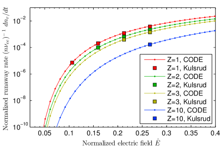
Figure 3: (Color online) Benchmark of CODE in the nonrelativistic limit $\delta\to 0$ against data in Table 1 of Ref. Kulsrud et al. (1973).

To emphasize the speed of CODE, we have directly compared it to the ARENA code Eriksson and Helander (2003) for computing the runaway rate using the parameters considered in Kulsrud et al. (1973). ARENA is a Monte Carlo code written in Fortran 90 and designed specifically to compute the runaway distribution function and runaway rate. Detailed description of the current version of ARENA is given in Refs. Rydén (2012); Csépány (2012). Both codes were run on a single thread on the same computer with an Intel Xeon 2.0 GHz processor. ARENA required 49,550 seconds to reproduce the left square point in figure 3, and 5,942 seconds to reproduce the top-right square point. 50,000 particles were required for reasonable convergence. For comparison, at a similar level of convergence, time-independent CODE required 0.00106 s and 0.000696 s for the two respective points, and time-dependent CODE required 0.0307 s and 0.00082 s respectively. Thus, for these parameters, both time-independent and time-dependent CODE require less than $1.5\times 10^{-7}$ as many cpu-hours as ARENA for the same hardware.

V Secondary runaway electron generation

In the previous sections we used the Fokker-Planck collision operator, which includes “distant” (large impact parameter) collisions but not “close” (small impact parameter) collisions in which a large fraction of energy and momentum are transferred between the colliding particles. Close collisions are infrequent compared to distant collisions, and are therefore neglected in the Fokker-Planck operator. However, close collisions may still have a significant effect on runaway generation, since the density of runaways is typically much smaller than the density of thermal electrons which may be accelerated in a close collision. The production of runaways through close collisions is known as secondary production, or as avalanche production since it may occur with exponential growth. To simulate secondary generation of energetic electrons, we use a source term derived in Rosenbluth and Putvinski (1997), starting from the Møller scattering cross-section in the $w\gg 1$ limit, with $w=p/(mc)=\delta y$ a normalized momentum. In this limit, the trajectories of the primary electrons are not much deflected by the collisions. The source then takes the form

$$S=\frac{n_{r}}{4\pi\tau\ln\Lambda}\delta(\xi-\xi_{2})\frac{1}{w^{2}}\frac{\partial}{\partial w}\left(\frac{1}{1-\sqrt{1+w^{2}}}\right),$$ (18)

where $1/\tau=4\pi ne^{4}\ln{\Lambda}/(m^{2}c^{3})$ is the collision frequency for relativistic electrons, $n_{r}$ is the density of the fast electrons and $\xi_{2}=w/(1+\sqrt{1+w^{2}})$ is the cosine of the pitch angle at which the runaway is born. (Our Eq. (18) differs by a factor $m^{3}c^{3}$ compared to the source in Ref. Rosenbluth and Putvinski (1997) since we normalize our distribution function as $n=\int d^{3}p\;f$ instead of $n=\int d^{3}w\;f$. There is also a factor of $2\pi$ difference due to the different normalization of the distribution function.)

Due to the approximations used to derive $S$, care must be taken in several regards. First, to define $n_{r}$ in (18), it is not clear where to draw the dividing line in velocity space between runaways and non-runaways. One possible strategy for defining $n_{r}$ is to compute the separatrix in velocity space between trajectories that will have bounded and unbounded energy in the absence of diffusion, and to define the runaway density as the integral of $f$ over the latter region Smith et al. (2005). This approach may somewhat overestimate the true avalanche rate, since it neglects the fact that some time must elapse between an electron entering the runaway region and the electron gaining sufficient energy to cause secondary generation. As most runaways have $\xi\approx 1$, we may approximate the separatrix by setting $dw/dt=0$ where $dw/dt=eE/(mc)-(1+1/w^{2})/\tau$ defines the trajectory of a particle with $\xi=1$, neglecting diffusion in momentum and pitch angle. The runaway region is therefore $w>w_{c}$ where $w_{c}=\left[(E/E_{c})-1\right]^{-1/2}$ and $E_{c}=mc/(e\tau)$ is the critical field, and so we take $n_{r}=2\pi m^{3}c^{3}\int_{-1}^{1}d\xi\int_{w_{c}}^{\infty}dw\;w^{2}f$. (We cannot define $n_{r}$ by the time integral of (17), since (17) is no longer valid when $S$ is nonzero away from $p\approx 0$.) A second deficiency of (18) is that $S$ is singular at $w\to 0$, so the source must be cut off below some threshold momentum. Following Ref. Harvey et al. (2000), we choose the cutoff to be $w_{c}$. Neither of the cutoffs discussed here would be necessary if a less approximate source term than (18) were used, but derivation of such an operator is beyond the scope of this paper.

Normalizing and applying (14) as we did previously for the other terms in the kinetic equation, the source included in CODE becomes

$$\hat{S}_{L}=\frac{n_{r}}{n}\frac{3\pi\delta^{5}}{16\ln\Lambda}\frac{2L+1}{2}P_{L}(\xi_{2})\frac{1}{(1-\sqrt{1+w^{2}})^{2}\sqrt{1+w^{2}}y}.$$ (19)

When secondary generation is included, CODE must be run in time-dependent mode.

To benchmark the numerical solution of the kinetic equation including the above source term by CODE, we use the approximate analytical expression for the avalanche distribution function derived in Section II of Ref. Fülöp et al. (2006):

$$f_{aa}(w_{\parallel},w_{\perp})=\frac{k}{w_{||}}\exp\left({\tilde{\gamma}}t-\frac{{\tilde{\gamma}}\tau}{E/E_{c}-1}w_{||}-\left[\frac{E/E_{c}-1}{Z+1}\right]\frac{w_{\perp}^{2}}{2w_{||}}\right)$$ (20)

where $k$ is a constant. The quantity ${\tilde{\gamma}}$ is the growth rate ${\tilde{\gamma}}=(1/f)\partial f/\partial t$, which must be independent of both time and velocity for (20) to be valid. Equation (20) is also valid only where $p_{||}\gg p_{\perp}$ and in regions of momentum space where $S$ is negligible. (This restriction is not a major one since $S=0$ everywhere except on the $\xi=\xi_{2}$ curve.) If most of the runaway distribution function is accurately described by (20), then we may approximate $n_{r}\approx\int d^{3}p\;f_{aa}=2\pi m^{3}c^{3}\int_{-\infty}^{\infty}dw_{\parallel}\int_{0}^{\infty}dw_{\perp}\;w_{\perp}f_{aa}$, giving ${\tilde{\gamma}}=(1/n_{r})dn_{r}/dt$ and

$$k=n_{r}e^{-{\tilde{\gamma}}t}\frac{\tau}{2\pi m^{3}c^{3}(1+Z)}$$ (21)

where $n_{r}e^{-{\tilde{\gamma}}t}$ is constant. (Equation (21) may be inaccurate in some situations even if (20) is accurate in part of velocity-space, because (21) requires (20) to apply in all of velocity-space.) Figures 4 and 5 show comparisons between distributions from CODE and (20)-(21) for two different sets of parameters. More precisely, the quantity plotted in figures 4-5 is $\log_{10}(m^{3}c^{3}f/n_{r})$. To generate the figures, CODE is run for a sufficiently long time that $(1/f)\partial f/\partial t$ becomes approximately constant. The resulting numerical value of $(1/n_{r})dn_{r}/dt$ is then used as ${\tilde{\gamma}}$ when evaluating (20)-(21). For a cleaner comparison between CODE and analytic theory in these figures, we minimize primary generation in CODE in these runs by initializing $f$ to 0 instead of to a Maxwellian. For both sets of physical parameters, the agreement between CODE and (20) is excellent in the region where agreement is expected: where $p_{||}\gg p_{\perp}$ and away from the curve $\xi=\xi_{2}$.

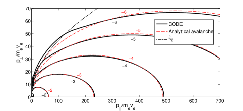
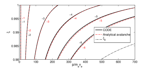
Figure 4: (Color online) Contour plots of the long-time distribution function from CODE (shown in two different coordinate systems), obtained for $E/E_{c}=40$ $(\hat{E}=0.532)$, $Z=3$, $\delta=0.1$ and $t=5000/\nu_{\mathrm{ee}}$. Results are plotted for the numerical parameters $N_{y}=1500$, $y_{max}=1500$ and $N_{\xi}=100$, with time step $dt=10/\nu_{\mathrm{ee}}$. The analytical distribution in (20)-(21) for the same physical parameters is also plotted for comparison, together with part of the curve where avalanche runaways are created ($\xi=\xi_{2}$).

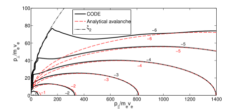
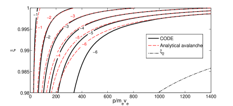
Figure 5: (Color online) Contour plots of the long-time distribution function from CODE (shown in two different coordinate systems), obtained for $E/E_{c}=100$ $(\hat{E}=0.332)$, $Z=1$, $\delta=0.05$ and $t=6000/\nu_{\mathrm{ee}}$. Results are plotted for the numerical parameters $N_{y}=1500$, $y_{max}=3000$ and $N_{\xi}=180$, with time step $dt=25/\nu_{\mathrm{ee}}$. The analytical distribution in (20)-(21) is also plotted for comparison, together with part of the curve where avalanche runaways are created ($\xi=\xi_{2}$).

VI Synchrotron emission

Using the distribution functions calculated with CODE, we now proceed to compute the spectrum of emitted synchrotron radiation. Due to the energy dependence of the emitted synchrotron power, the emission from runaways completely dominates that of the thermal particles. The emission also depends strongly on the pitch-angle of the particle. In a cylindrical plasma geometry, the emitted synchrotron power per wavelength at wavelength $\lambda$ from a single highly energetic particle is given by Bekefi (1966)

$$\quad\mathcal{P}(\gamma,\gamma_{\|},\lambda)=\frac{4\pi}{\sqrt{3}}\,\frac{ce^{2}}{\lambda^{3}\gamma^{2}}\int_{\lambda_{c}/\lambda}^{\infty}\!\!\!K_{5/3}(l)\,dl\ ,\quad$$ (22)

where the two-dimensional momentum of the particle is determined by $\gamma$ and $\gamma_{\|}=1/\sqrt{1-v_{\|}^{2}/c^{2}}$, $K_{\nu}(x)$ is a modified Bessel function of the second kind, and

$$\lambda_{c}=\frac{4\pi}{3}\frac{mc^{2}\gamma_{\parallel}}{eB\gamma^{2}}\ ,$$ (23)

where $B$ is the magnetic field strength.

Using CODE we will demonstrate that the synchrotron radiation spectrum from the entire runaway distribution is substantially different from the spectrum obtained from a single particle approximation. By transforming to the more suitable coordinates $w$ and $\xi$, related to $\gamma$ and $\gamma_{\|}$ through $\gamma^{2}=1+w^{2}$ and $\gamma_{\|}^{2}=(1-w^{2}\xi^{2}/(1+w^{2}))^{-1}$, and integrating (22) over the runaway region $R$ in momentum space, we obtain the total synchrotron emission from the runaway distribution. Normalizing to $n_{r}$, we find that the average emitted power per runaway particle at a wavelength $\lambda$ is given by

$$P(\lambda)=\frac{2\pi}{n_{r}}\int_{R}f(w,\xi)\,\mathcal{P}(w,\xi,\lambda)\,w^{2}\mbox{d}w\,\mbox{d}\xi\ .$$ (24)

Up to a factor $ecA$, where $A$ is the area of the runaway beam, normalization by $n_{r}$ is equivalent to normalization by the runaway current, since the emitting particles all move with velocity $\approx c$.

The per-particle synchrotron spectra generated by the CODE distributions in Figures 4 and 5 were calculated using this formula, and are shown in Figure 6, together with the spectra radiated by electron distributions for other electric field strengths. For the physical parameters used, we note that the peak emission occurs between 7 and 25 $\mu$m. The synchrotron spectra show a decrease in per-particle emission with increasing electric field strength. Even though a stronger electric field leads to more particles with high energy (and thus high average emission), it also leads to a more narrow distribution in pitch-angle. This reduction in the number of particles with large pitch-angle leads to a decrease in average emission. Both figures confirm that the average emission is reduced for higher electric fields, implying that the latter mechanism has the largest impact on the spectrum.

In calculating the spectra, the runaway region of momentum space, $R$, was defined such that the maximum particle momentum was $w_{\text{max}}=50$ (which translates to $y_{\text{max}}=500$ and $y_{\text{max}}=1000$ respectively for the cases shown in Figures 4 and 5), corresponding to a maximum particle energy of $\simeq 25$ MeV. Physically the cutoff at large energy can be motivated by the finite life-time of the accelerating electric field and the influence of loss mechanisms such as radiation. Since the radiated synchrotron power increases with both particle energy and pitch, this truncation of the distribution is necessary to avoid infinite emission, although the precise value for the cutoff depends on the tokamak and on discharge-specific limitations to the maximum runaway energy. For the low-energy boundary of $R$, $w_{\text{min}}=w_{c}=\left[(E/E_{c})-1\right]^{-1/2}$ was used, and all particles with $\xi\in[0,1]$ were included. Although no explicit cutoff was imposed in $\xi$, the distribution decreases rapidly as this parameter decreases from 1 (as can be seen in Figures 4 and 5) and there are essentially no particles below some effective cutoff value.

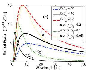
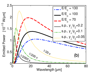
Figure 6: (Color online) Synchrotron spectra (average emission per particle) for the runaway distributions in (a) Figure 4 and (b) Figure 5. Emission spectra from the CODE distributions in Figures 4 and 5 are shown in solid black, together with spectra from distributions with varying electric field strength but otherwise identical physical parameters. A magnetic field of $B=3\,$T was used. The synchrotron spectra from single particles with $w=50$ and various pitch angles are also shown. (These single-particle spectra are the same in figures a and b, as the particle parameters are independent of simulation settings).

Figure 6 also shows the synchrotron spectrum from single particles with momentum corresponding to the maximum momentum of the distributions ($w=50$), and several values of pitch-angle $y_{\perp}/y_{\|}$. This single-particle “approximation” is equivalent to using a 2D $\delta$-function model of the distribution, as was done in Refs. Finken et al. (1990); Jaspers et al. (2001) (and with some modification in Yu et al. (2013)). The figure shows that this approximation significantly overestimates the synchrotron emission per particle. Note that in the figure, the values for the emitted power per particle were divided by a large number to fit in the same scale. The overestimation is not surprising, since the $\delta$-function approximation effectively assumes that all particles emit as much synchrotron radiation as one of the most strongly emitting particle in the actual distribution. The figure also shows that the $\delta$-function approximation leads to a different spectrum shape, with the wavelength of peak emission usually shifted towards shorter wavelengths. In order to obtain an accurate runaway synchrotron spectrum, it is thus crucial to use the full runaway distribution in the calculation.

In the cases shown in Fig. 6, the runaway electron distribution is dominated by secondary generation. For comparison, in Figs. 7-8 we show a case where the distribution is dominated by primary generation. Figure 7a shows contours of a distribution from primaries only, together with a distribution obtained with the avalanche source enabled, and confirms that the distribution is dominated by primaries, except for a small number of secondary runaways generated along the curve $\xi=\xi_{2}$. Fig. 7b shows contour plots with the avalanche source enabled, for three different times. The physical parameters used in Fig. 7 are temperature $T=10\;\rm keV$, density $n=5\times 10^{19}\;\rm m^{-3}$, effective charge $Z=1$, and electric field $E=0.45\;\rm V/m$. The collision time in this case is $0.39\;\rm ms$, so the times shown in the figure correspond to $5.9\;\rm ms$, $11.8\;\rm ms$ and $17.6\;\rm ms$, which correlates well with the time-scale of the electric field spike for a typical disruption in DIII-D (see e.g. Fig. 2 in Hollmann et al. (2013).) Figure 8 compares the synchrotron spectra from the distributions shown in Fig. 7. The main difference compared to the case dominated by secondary generation (Fig. 6) is the generally longer wavelengths in the spectrum. The reason is the low runaway electron energy ($w\mathrel{\mbox{\raisebox{-2.84526pt}{$\stackrel{{\scriptstyle<}}{{\sim}}$}}}10$) in the runaway electron distribution in this case. The small peak at short wavelengths in the spectra including the avalanche source stems from the secondary runaways generated at $\xi=\xi_{2}$ (visible in Fig. 7a).

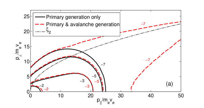
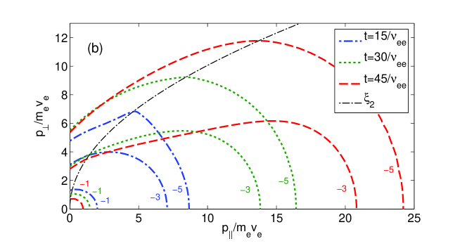
Figure 7: (Color online) (a) Contour plots of the distribution function from primaries only (black solid line), together with a distribution obtained with the avalanche source enabled (dashed red line), for $E/E_{c}=10$ $(\hat{E}=0.523)$, $Z=1$ and $\delta=0.2$ at $t=45/\nu_{ee}$. The quantity plotted is $\log_{10}(F)$. Results are plotted for the numerical parameters $N_{y}=20$, $y_{max}=100$ and $N_{\xi}=130$, with time step $dt=0.02/\nu_{ee}$. (b) Contour plots of the distribution function at different times with the avalanche source enabled, using the above parameters.

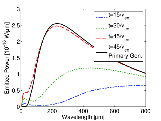
Figure 8: (Color online) Synchrotron spectra (average emission per particle) for the runaway distributions shown in Fig. 7 for magnetic field $B=3\,$T.

In principle, we may also use the synchrotron spectra from distributions calculated through CODE to estimate the maximum energy of the runaways in existing tokamaks. However, due to the region of sensitivity of the available detectors, there is only a limited wavelength range in which calculated spectra can be fitted to experimental data in order to determine the maximum runaway energy. The available range often corresponds to the short wavelength slope of the spectrum, where the emitted power shows an approximately linear dependence on wavelength. Indeed, the short-wavelength spectrum slope has been used to estimate the maximum runaway energy in experiments (Jaspers et al., 2001). If the runaway distribution function is approximated by a $\delta$-function at the maximum available energy and pitch angle, there is a monotonic relationship between the short-wavelength spectrum slope and the maximum particle energy (at fixed pitch angle). Such a relationship holds because increasing the particle energy leads to more emission at shorter wavelengths, resulting in a shift of the wavelength of peak emission towards shorter wavelengths, and a corresponding change in the spectrum slope.

Using an integrated synchrotron spectrum from a CODE distribution is much more accurate than the single particle approximation, but it also introduces additional parameters ($\hat{E}$, $\delta$, $Z$). If the physical parameters are well known, a unique relation still holds between the spectrum slope and the maximum particle energy. During disruptions however, many parameters (like the temperature and the effective charge) are hard to measure with accuracy. As the shape of the underlying distribution depends on the values of the parameters, the synchrotron spectrum will do so as well. This complexity is apparent in Figure 6, where the single particle approximation produces identical results in the two cases, whereas the spectra from the complete distributions are widely different. The dependence on distribution shape makes it possible in principle for two sets of parameters to produce the same spectrum slope for different maximum energies. Given this insight, using the complete runaway distribution when modeling experimentally obtained spectra is necessary for an accurate analysis and reliable fit of the maximum particle energy. In this context, CODE is a very useful tool with the possibility to contribute to the understanding of runaways and their properties.

VII Conclusions

In this work, we have computed the synchrotron emission spectra from distribution functions of runaway electrons. The distribution functions are computed efficiently using the CODE code. Both primary (Dreicer) and secondary (avalanche) generation are included. A Legendre spectral discretization is applied to the pitch-angle coordinate, with high-order finite differences applied to the speed coordinate. A nonuniform speed grid allows high resolution of thermal particles at the same time as a high maximum energy without a prohibitively large number of grid points. If secondary generation is unimportant, the long-time distribution function may be calculated by solving a single sparse linear system. The speed of the code makes it feasible to couple to other codes for integrated modeling of complex processes such as tokamak disruptions. CODE has been benchmarked against previous analytic and numerical results in appropriate limits, showing excellent agreement. In the limit of strong avalanching, CODE demonstrates agreement with the analytic distribution function (20) from Ref. Fülöp et al., 2006.

The synchrotron radiation spectra are computed by convolving the distribution function with the single-particle emission. We find that the radiation spectrum from a single electron at the maximum energy can differ substantially from the overall spectrum generated by a distribution of electrons. Therefore, experimental estimates of maximum runaway energy based on the single-particle synchrotron spectrum are likely to be inaccurate. A detailed study of the distribution-integrated synchrotron spectrum and its dependence on physical parameters can be found in Ref. Stahl et al. (2013).

In providing the electron distribution functions (and thus knowledge of a variety of quantities through its moments), the applicability of CODE is wide, and the potential in coupling CODE to other software, e.g. for modeling of runaway dynamics in disruptions, is promising. For a proper description of the runaways generated in disruptions it is important to take into account the evolution of the radial profiles of the electric field and fast electron current self-consistently. This can be done by codes such as GO, initially described in Ref. Smith et al. (2006) and developed further in Refs. Gál et al. (2008); Fehér et al. (2011). GO solves the equation describing the resistive diffusion of the electric field in a cylindrical approximation coupled to the runaway generation rates. In the present version of GO, the runaway rate is computed by approximate analytical formulas for the primary and secondary generation. Using CODE, the analytical formulas can be replaced by a numerical solution for the runaway rate which would have several advantages. One advantage would be that Dreicer, hot-tail and secondary runaways could all be calculated with the same tool, avoiding the possibilities for double-counting and difficulties with interpretations of the results. Also, in the present version of GO, it is assumed that all the runaway electrons travel at the speed of light, an approximation that can be easily relaxed using CODE, which calculates the electron distribution in both energy and pitch-angle. Most importantly, the validity region of the results would be expanded, as the analytical formulas are derived using various assumptions which are often violated in realistic situations. The output would be a self-consistent time and space evolution of electric field and runaway current, together with the electron distribution function. This information can then be used for calculating quantities that depend on the distribution function, such as the synchrotron emission or the kinetic instabilities driven by the velocity anisotropy of the runaways.

Appendix A Integrals of Legendre Polynomials

Here we list several identities for Legendre polynomials which are required for the spectral pitch-angle discretization. To evaluate the $\xi$ integral of the $\xi\;\partial F/\partial y$ term in (11), we use the recursion relation

$$\xi\;P_{L}(\xi)=\frac{L+1}{2L+1}P_{L+1}(\xi)+\frac{L}{2L+1}P_{L-1}(\xi)$$ (25)

where $P_{L-1}$ is replaced by 0 when $L=0$. Applied to the relevant integral in (11), and noting the orthogonality relation $(2L+1)2^{-1}\int_{-1}^{1}P_{L}(\xi)P_{\ell}(\xi)d\xi=\delta_{L,\ell}$, we find

$$\frac{2L+1}{2}\int_{-1}^{1}d\xi\;\xi\;P_{L}(\xi)P_{\ell}(\xi)=\frac{L+1}{2L+3}\delta_{\ell,L+1}+\frac{L}{2L-1}\delta_{\ell,L-1}.$$ (26)

Similarly, to evaluate the $\xi$ integral of the $\partial F/\partial\xi$ term in (11), we use the recursion relation

$$(1-\xi^{2})(dP_{L}/d\xi)=LP_{L-1}(\xi)-L\xi P_{L}(\xi)$$ (27)

to obtain

$$\frac{2L+1}{2}\int_{-1}^{1}d\xi\;P_{L}(\xi)(1-\xi^{2})\frac{dP_{\ell}}{d\xi}=\frac{(L+1)(L+2)}{2L+3}\delta_{\ell,L+1}-\frac{(L-1)L}{2L-1}\delta_{\ell,L-1}.$$ (28)

Finally, the pitch-angle scattering collision term gives the integral

$$\frac{2L+1}{2}\int_{-1}^{1}d\xi\;P_{L}(\xi)\frac{\partial}{\partial\xi}(1-\xi^{2})\frac{\partial}{\partial\xi}P_{\ell}(\xi)=-(L+1)L\delta_{L,\ell}.$$ (29)

References

- Dreicer (1960) H. Dreicer, Phys. Rev. 117, 329 (1960).
- Connor and Hastie (1975) J. W. Connor and R. J. Hastie, Nucl. Fusion 15, 415 (1975).
- Furth and Rutherford (1972) H. P. Furth and P. H. Rutherford, Phys. Rev. Lett. 28, 545 (1972).
- Helander and Ward (2003) P. Helander and D. Ward, Phys. Rev. Lett. 90, 135004 (2003).
- Fülöp and Papp (2012) T. Fülöp and G. Papp, Phys. Rev. Lett. 51, 043004 (2012).
- Papp et al. (2011) G. Papp, M. Drevlak, T. Fülöp, and P. Helander, Nucl. Fusion 51, 043004 (2011).
- Martín-Solís et al. (1998) J. R. Martín-Solís, J. D. Alvarez, R. Sánchez, and B. Esposito, Phys. Plasmas 5, 2370 (1998).
- Heikkinen et al. (1993) J. A. Heikkinen, S. K. Sipilä, and T. J. H. Pättikangas, Comp. Phys. Comm. 76, 215 (1993).
- Eriksson and Helander (2003) L.-G. Eriksson and P. Helander, Comp. Phys. Comm. 154, 175 (2003).
- O’Brien et al. (1986) M. R. O’Brien, M. Cox, and D. F. H. Start, Nucl. Fusion 26, 1625 (1986).
- Chiu et al. (1998) S. C. Chiu, M. N. Rosenbluth, R. W. Harvey, and V. S. Chan, Nucl. Fusion 38, 1711 (1998).
- Harvey et al. (2000) R. W. Harvey, V. S. Chan, S. C. Chiu, T. E. Evans, and M. N. Rosenbluth, Phys. Plasmas 7, 4590 (2000).
- Peysson et al. (2003) Y. Peysson, J. Decker, and R. W. Harvey, AIP Conf. Proc. 694, 495 (2003).
- Peysson and Decker (2008) Y. Peysson and J. Decker, AIP Conf. Proc. 1069, 176 (2008).
- Karney and Fisch (1986) C. Karney and N. Fisch, Phys. Fluids 29, 180 (1986).
- Jaspers et al. (2001) R. Jaspers, N. J. L. Cardozo, A. J. H. Donné, H. L. M. Widdershoven, and K. H. Finken, Rev. Sci. Instrum. 72, 466 (2001).
- Yu et al. (2013) J. H. Yu, E. M. Hollmann, N. Commaux, N. W. Eidietis, D. A. Humphreys, A. N. James, T. C. Jernigan, and R. A. Moyer, Phys. Plasmas 20, 042113 (2013).
- Fülöp et al. (2006) T. Fülöp, G. Pokol, P. Helander, and M. Lisak, Phys. Plasmas 13, 062506 (2006).
- Rosenbluth and Putvinski (1997) M. N. Rosenbluth and S. V. Putvinski, Nucl. Fusion 37, 1355 (1997).
- Sandquist et al. (2006) P. Sandquist, S. E. Sharapov, P. Helander, and M. Lisak, Phys. Plasmas 13, 072108 (2006).
- Karney and Fisch (1985) C. Karney and N. Fisch, Phys. Fluids 28, 116 (1985).
- Karney and Fisch (1979) C. Karney and N. Fisch, Phys. Fluids 22, 1817 (1979).
- Kulsrud et al. (1973) R. M. Kulsrud, Y.-C. Sun, N. K. Winsor, and H. A. Fallon, Phys. Rev. Lett. 31, 690 (1973).
- Rydén (2012) J. Rydén, Master’s thesis, Chalmers University of Technology (2012), http://publications.lib.chalmers.se/records/fulltext/179211/179211.pdf.
- Csépány (2012) G. Csépány, Master’s thesis, Budapest University of Technology and Economics (2012), http://deep.reak.bme.hu/~cheoppy/diploma-thesis-2012.pdf.
- Smith et al. (2005) H. Smith, P. Helander, L.-G. Eriksson, and T. Fülöp, Phys. Plasmas 12, 122505 (2005).
- Bekefi (1966) G. Bekefi, Radiation Processes in Plasmas (Wiley, 1966).
- Finken et al. (1990) K. H. Finken, J. G. Watkins, D. Rusbuldt, W. J. Corbett, K. H. Dippel, D. M. Goebel, and R. A. Moyer, Nucl. Fusion 30, 859 (1990).
- Hollmann et al. (2013) E. M. Hollmann, M. E. Austin, J. A. Boedo, N. H. Brooks, N. Commaux, N. W. Eidietis, D. A. Humphreys, V. A. Izzo, A. N. James, T. C. Jernigan, et al., Nucl. Fusion 53, 083004 (2013).
- Stahl et al. (2013) A. Stahl, M. Landreman, G. Papp, E. Hollmann, and T. Fülöp, Phys. Plasmas 20, 093302 (2013).
- Smith et al. (2006) H. Smith, P. Helander, L.-G. Eriksson, D. Anderson, M. Lisak, and F. Andersson, Phys. Plasmas 13, 102502 (2006).
- Gál et al. (2008) K. Gál, T. Fehér, H. Smith, T. Fülöp, and P. Helander, Plasma Phys. Controlled Fusion 50, 055006 (2008).
- Fehér et al. (2011) T. Fehér, H. M. Smith, T. Fülöp, and K. Gál, Plasma Phys. Controlled Fusion 53, 035014 (2011).