Applying electric field to charged and polar particles between metallic plates: Extension of the Ewald method

Abstract

We develop an efficient Ewald method of molecular dynamics simulation for calculating the electrostatic interactions among charged and polar particles between parallel metallic plates, where we may apply an electric field with an arbitrary size. We use the fact that the potential from the surface charges is equivalent to the sum of those from image charges and dipoles located outside the cell. We present simulation results on boundary effects of charged and polar fluids, formation of ionic crystals, and formation of dipole chains, where the applied field and the image interaction are crucial. For polar fluids, we find a large deviation of the classical Lorentz-field relation between the local field and the applied field due to pair correlations along the applied field. As general aspects, we clarify the difference between the potential-fixed and the charge-fixed boundary conditions and examine the relationship between the discrete particle description and the continuum electrostatics.

I Introduction

In many problems in physics and chemistry, the electrostatic potential and field acting on each constituting particle need to be calculated Is . A large number of simulations have been performed to accurately estimate the long-range electrostatic interactions among charged and polar particles Allen ; Frenkel . The Ewald method is a famous technique for efficiently summing these interactions using the Fourier transformation. It was originally devised for ionic crystals Ewald and has been widely used to investigate bulk properties of charged and polar particles under the periodic boundary condition in three dimensions (3D) Leeuw ; Leeuwreview ; Weis ; Mazars . It has also been modified for filmlike systems bounded by non-polarizable and insulating regions under the periodic boundary condition in the lateral directions Frenkel ; Parry ; Smith ; Crozier ; Yeh ; KlappJCP ; Tyagi ; Smith1 .

However, the Ewald method has not yet been successful when charged or polar particles are in contact with metallic or polarizable plates and when electric field is applied from outside. Such situations are ubiquitous in solids and soft matters. In idealized metallic plates, the surface charges spontaneously appear such that the electrostatic potential is homogeneous within the plates, thus providing the well-defined boundary condition for the potential within the cell Landau . Between two parallel plates, we may control the potential difference to apply an electric field. However, the electrostatic interaction between the surface charges and the particles within the cell is highly nontrivial. On the other hand, such surface changes are nonexistent for the magnetic interaction.

Each charged particle between parallel metallic plates induces surface charges producing a potential equivalent to that from an infinite number of image charges outside the cell. If a charged particle approaches a metal wall, it is attracted by the wall or by its nearest image. Some mathematical formulae including these image charges in the Ewald sum were presented by Hautman et al.Hautman and by Perram and Ratner Perram . In the same manner, for each dipole in the cell, an infinite number of image dipoles appear. A dipole close to a metal surface is attracted and aligned by its nearest image. Accounting for these image dipoles, Klapp Klapp performed Monte Carlo simulations of 500 dipoles interacting with the soft-core potential, but without applied electric field, to find wall-induced ordering. The image effect is also relevant in electrorheological fluids between metallic plates Hasley ; Tao .

Inclusion of the image effect in molecular dynamics simulations of molecules near a conducting or polarizable surface is still challenging in a variety of important systems including proteins Corni , polyelectrolytes Messina , and colloidal particles colloid . Moreover, the effects of applied electric field remain largely unexplored on the microscopic level, while the continuum electrostatics is well established Landau ; OnukiNATO . For example, the local electric field acting on a dipole is known to be different from the applied electric field in dielectrics and polar fluids Onsager ; Kirk , where the difference is enlarged in highly polarizable systems. In contrast, a number of microscopic simulations have been performed on the effect of uniform magnetic field for systems of magnetic dipoles magnetic ; Weis ; Mazars .

In this paper, we hence aim to develop an efficient Ewald method to treat charged and polar particles between parallel metallic plates accounting for the image effect, where we apply an electric field with an arbitrary size. In the Ewald sum in this case, we can sum up the terms homogeneous in the lateral $xy$ plane but inhomogeneous along the normal $z$ axis into a simple form and can calculated them precisely. This one-dimensional part of the electrostatic energy yields one-dimensional (laterally averaged) electric field along the $z$ axis for each particle.

Using our scheme, we present some numerical results under applied electric field, including the soft-core pair interaction and the wall-particle repulsive interaction. We confirm that accumulation of charges and dipoles near metallic walls gives rise to a uniaxially symmetric, homogeneous interior region. We also examine formation of ionic crystals super and that of dipole chains Hasley ; Tao ; PG under electric field. Here, we are interested in the mechanisms of dipole alignment near metallic walls, which are caused by the image interaction or by the applied electric field. We shall also see that the classical local field relation Onsager ; Kirk is much violated in our dipole systems because of strong pair correlations along the applied field.

The organization of this paper is as follows. In Sec.II, we will extend the Ewald scheme for charged particles between metallic plates. In Sec.III, we will further develop the Ewald scheme for point-like dipoles between metallic plates. In these two sections, we will present some numerical results. In Appendix B, we will clarify the difference between two boundary conditions at a fixed potential difference and at fixed surface charges. In Appendix D, we will compare the electrostatics of our discrete particle systems and the continuum electrostatics.

II Charged particles

We consider $N$ charged particles in a cell. Their positions and charges are ${\mbox{\boldmath$r$}}_{i}$ and $q_{i}$ ($1\leq i\leq N)$. We assume the charge neutrality condition,

$$\sum_{i}q_{i}=0.$$ (2.1)

In terms of the electrostatic energy $U=U({\mbox{\boldmath$r$}}_{1},\cdots,{\mbox{\boldmath$r$}}_{N})$, the electrostatic force on particle $i$ is given by

$${\mbox{\boldmath$F$}}_{i}^{e}=q_{i}{\mbox{\boldmath$E$}}_{i}=-\frac{\partial}{\partial{\mbox{\boldmath$r$}}_{i}}U,$$ (2.2)

where ${\mbox{\boldmath$E$}}_{i}$ is the electric field on particle $i$. There can also be neutral particles interacting with charged ones.

II.1 Ewald method for charged particles in the periodic boundary condition

When the bulk properties of charged particle systems are calculated, the periodic boundary condition is usually assumed in molecular dynamics simulation. In a $L\times L\times L$ cell, the electrostatic energy is written as Allen ; Frenkel

$$U_{\rm p}=\frac{1}{2}\sum_{\mbox{\boldmath$m$}}{\sum_{i,j}}^{\prime}\frac{q_{i}q_{j}}{|{\mbox{\boldmath$r$}}_{ij}+L{\mbox{\boldmath$m$}}|},$$ (2.3)

where ${\mbox{\boldmath$r$}}_{ij}={\mbox{\boldmath$r$}}_{i}-{\mbox{\boldmath$r$}}_{j}$ is the relative positional vector, ${\mbox{\boldmath$m$}}=(m_{x},m_{y},m_{z})$ is a 3D vector with three integer components, and the self terms ($j=i$ and ${\mbox{\boldmath$m$}}={(0,0,0)}$) are excluded in the summation ${\sum_{i,j}}^{\prime}$. Here, ${\mbox{\boldmath$E$}}_{i}$ is obtained from Eq.(2.2) with $U=U_{\rm p}$. In some papersTyagi ; Smith1 , discussions have been made on the convergence of the Ewald sum under Eq.(2.1).

In the Ewald method, the Coulomb potential $q_{i}q_{j}/r$ is divided into the short-range part $q_{i}q_{j}\psi_{s}(r)$ and the long-range part $q_{i}q_{j}\psi_{\ell}(r)$, where

$$\psi_{s}(r)={\rm erfc}(\gamma r)\frac{1}{r},\quad\psi_{\ell}(r)={\rm erf}(\gamma r)\frac{1}{r}.$$ (2.4)

Here, ${\rm erf}(u)=(2/\sqrt{\pi})\int_{0}^{u}due^{-u^{2}}$ is the error function and ${\rm erfc}(u)=1-{\rm erf}(u)$ is the complementary error function. The function $\psi_{\ell}(r)$ is the solution of $\nabla^{2}\psi_{\ell}(r)=-4\pi\varphi_{3}(r)$, where $\varphi_{3}(r)=\varphi(x)\varphi(y)\varphi(z)$ is a normalized 3D Gaussian distribution with

$$\varphi(x)=(\gamma/\sqrt{\pi})\exp(-\gamma^{2}x^{2}).$$ (2.5)

The inverse $\gamma^{-1}$ is an adjustable potential range. For $r\gg\gamma^{-1}$, we have $\psi_{\ell}\cong r^{-1}$. For $r\ll\gamma^{-1}$ it is finite as

$$\psi_{\ell}(r)=(2\gamma/\sqrt{\pi})(1-\gamma^{2}r^{2}/3\cdots).$$ (2.6)

As is well-known Allen ; Frenkel , the Ewald form of $U_{\rm p}$ reads

$$U_{\rm p}=\sum_{\mbox{\boldmath$m$}}{\sum_{i,j}}^{\prime}\frac{q_{i}q_{j}}{2}\psi_{s}({|{\mbox{\boldmath$r$}}_{ij}+L{\mbox{\boldmath$m$}}|})-\sum_{i}\frac{\gamma q_{i}^{2}}{\sqrt{\pi}}$$

$$+\frac{1}{L^{3}}{\sum_{{\mbox{\boldmath$\nu$}}\neq{\mbox{\boldmath$0$}}}}\sum_{i,j}\frac{q_{i}q_{j}}{2}\Psi_{\ell}(k)e^{{\rm i}{\mbox{\boldmath$k$}}\cdot{\mbox{\boldmath$r$}}_{ij}}+\frac{2\pi}{3L^{3}}\bigg{|}\sum_{i}q_{i}{\mbox{\boldmath$r$}}_{i}\bigg{|}^{2},$$ (2.7)

where the second term is equal to $-\sum_{i}q_{i}^{2}\psi_{\ell}(0)/2$ and the last two terms arise from $\sum_{\mbox{\boldmath$m$}}{\sum_{i,j}}{q_{i}q_{j}}\psi_{\ell}({|{\mbox{\boldmath$r$}}_{ij}+L{\mbox{\boldmath$m$}}|})/2$ including the self part. Use is made of the Fourier transformation $\psi_{\ell}(r)=(2\pi)^{-3}\int d{\mbox{\boldmath$k$}}\Psi_{\ell}(k)\exp[{{\rm i}{\mbox{\boldmath$k$}}\cdot{\mbox{\boldmath$r$}}}]$, where

$$\Psi_{\ell}(k)=4\pi\exp(-k^{2}/4\gamma^{2})/k^{2}.$$ (2.8)

In the third term, $k$ is discretized as

$${\mbox{\boldmath$k$}}=(2\pi/L)(\nu_{x},\nu_{y},\nu_{z}),$$ (2.9)

and the term with ${\mbox{\boldmath$\nu$}}=(\nu_{x},\nu_{y},\nu_{z})={(0,0,0)}$ is excluded, where $\nu_{x}$, $\nu_{y}$, and $\nu_{z}$ are integers ($0,\pm 1,\pm 2,\cdots$). This discretization stems from the summation over $m$ in Eq.(2.3). The last term in Eq.(2.7) arises from the $k$-integration at small $|{\mbox{\boldmath$k$}}|\lesssim L^{-1}$. However, it is negligible without overall polarization or for $\sum_{i}q_{i}{\mbox{\boldmath$r$}}_{i}\cong{\mbox{\boldmath$0$}}$. See Appendix A for the derivation of the last two terms.

II.2 Ewald method for charged particles between metallic plates under applied electric field

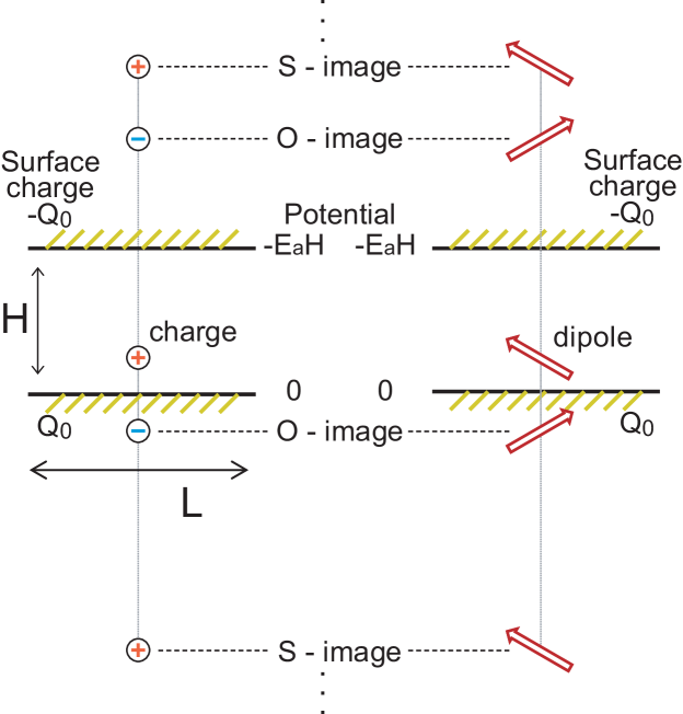
As in Fig.1, we consider a $L\times L\times H$ parallel plate geometry, where the plates at $z=0$ and $H$ are both metallic. They are assumed to be smooth and structureless. We assume the periodic boundary condition along the $x$ and $y$ axes. We adopt the fixed-potential boundary condition. See Appendix B for discussions of another typical boundary condition with fixed surface charges.

We treat an infinite number of image charges. Let a particle $i$ at ${\mbox{\boldmath$r$}}_{i}=(x_{i},y_{i},z_{i})$ with charge $q_{i}$ approach the surface at $z=0$. For not strong applied electric field, it is acted by a growing attractive force produced by the closest image with the opposite charge $-q_{i}$ at Landau ,

$${\bar{\mbox{\boldmath$r$}}}_{i}=(x_{i},y_{i},-z_{i}).$$ (2.10)

This force is written as $-\partial v_{\rm I}/\partial z_{i}=-q_{i}^{2}/(2z_{i})^{2}$ for small $z_{i}$, so the potential due to this image is of the form,

$$v_{\rm I}(z_{i})=-q_{i}^{2}/4z_{i}.$$ (2.11)

Figure 1: (Color online) System of a capacitor with parallel metallic plates containing charges (left) and dipoles (right). For each charge or dipole at $(x_{j},y_{j},z_{j})$, there appear O-images at $(x_{j},y_{j},-z_{j}-2Hn)$ ($n=0,\pm 1,\cdots)$ and S-images at $(x_{j},y_{j},z_{j}-2Hn)$ ($n=\pm 1,\cdots)$. The electrostatic potential $\Phi$ is $0$ at the bottom and is $-\Delta\Phi=-E_{a}H$ at the top. The surface charge is $Q_{0}$ at the bottom and $-Q_{0}$ at the top. As typical experiments, we may fix either of $\Delta\Phi$ or $Q_{0}$.

II.2.1 Electrostatic potential and image charges

We write the electrostatic potential away from the particle positions $({\mbox{\boldmath$r$}}\neq{\mbox{\boldmath$r$}}_{j}$) as

$$\Phi({\mbox{\boldmath$r$}})=\phi({\mbox{\boldmath$r$}})-E_{a}z.$$ (2.12)

The electric field away from the particle positions is ${\mbox{\boldmath$E$}}=E_{a}{\mbox{\boldmath$e$}}_{z}-\nabla\phi$, where ${\mbox{\boldmath$e$}}_{z}$ is the unit vector along the $z$ axis. We assume that the charged particles are repelled from the walls at short distances and that no ionization occurs on the walls. Then, the excess potential $\phi$ in Eq.(2.12) satisfies the boundary condition,

$$\phi(x,y,0)=\phi(x,y,H)=0.$$ (2.13)

From the bottom to the top, the potential difference is

$$\Delta\Phi=\Phi(x,y,0)-\Phi(x,y,H)=HE_{a}.$$ (2.14)

In the region $0<z<H$, $\phi({\mbox{\boldmath$r$}})$ is the solution of the Poisson equation under the boundary condition (2.13),

$$-\nabla^{2}\phi=4\pi\sum_{j}q_{j}\delta({\mbox{\boldmath$r$}}-{\mbox{\boldmath$r$}}_{j}).$$ (2.15)

To calculate $\phi({\mbox{\boldmath$r$}})$, we consider its 2D Fourier expansion,

$$\phi=\frac{4\pi}{L^{2}}\sum_{{\mbox{\boldmath$\nu$}}_{\perp}}\sum_{j}q_{j}G_{k}(z,z_{j})e^{{\rm i}\cdot(k_{x}(x-x_{j})+k_{y}(y-y_{j}))},$$ (2.16)

where ${\mbox{\boldmath$\nu$}}_{\perp}=(\nu_{x},\nu_{y})$ and $(k_{x},k_{y})=(2\pi/L)(\nu_{x},\nu_{y})$ with $\nu_{x}$ and $\nu_{y}$ being integers. From Eq.(2.15) the Green function $G_{k}(z,z^{\prime})$ satisfies

$$(k^{2}-\partial^{2}/\partial z^{2})G_{k}(z,z^{\prime})=\delta(z-z^{\prime}),$$ (2.17)

where $k=(k_{x}^{2}+k_{y}^{2})^{1/2}$. Here, $G_{k}(0,z^{\prime})=G_{k}(H,z^{\prime})=0$ from Eq.(2.13), so we solve Eq.(2.17) as OnukiNATO ; Perram

$$G_{k}(z,z^{\prime}) = \frac{1}{2k}e^{-k|z-z^{\prime}|}-\frac{1}{2k\sinh(kH)}$$ (2.18)

$$\times\bigg{[}\sinh(kz)e^{-k(H-z^{\prime})}+\sinh(kH-kz)e^{-kz^{\prime}}\bigg{]},$$

which has the symmetry $G_{k}(z,z^{\prime})=G_{k}(z^{\prime},z)$. The first term in Eq.(2.18) arises from the 2D Fourier transformation of the direct Coulombic interaction, while the second term is induced by the surface charges on the metallic surfaces. Note that the term with $k_{x}=k_{y}=0$ is included in Eq.(2.16), which give rise to a term independent of $x$ and $y$. From Eq.(2.18) the long wavelength limit $G_{0}(z,z^{\prime})=\lim_{k\rightarrow 0}G_{k}(z,z^{\prime})$ becomes

$$G_{0}(z,z^{\prime})=(z+z^{\prime}-|z-z^{\prime}|)/2-zz^{\prime}/H.$$ (2.19)

To find image charges, we further use the expansion $1/\sinh(kH)=2\sum_{n\geq 0}e^{-kH(2n+1)}$ in Eq.(2.18) to obtain

$$G_{k}(z,z^{\prime})=\frac{1}{2k}\sum_{n}\bigg{[}e^{-k|z-z^{\prime}+2Hn|}-e^{-k|z+z^{\prime}+2Hn|}\bigg{]},$$ (2.20)

where $n=0,\pm 1,\pm 2,\cdots$. Since $2\pi\exp({-k|z|})/k=\int dxdy\exp(ik_{x}x+ik_{y}y)/r$, substitution of the above expansion into Eq.(2.16) yields $\phi({\mbox{\boldmath$r$}})$ in the following superposition of Coulomb potentials,

$$\phi=\sum_{{\mbox{\boldmath$m$}}}{\sum_{j}}\frac{q_{j}}{|{\mbox{\boldmath$r$}}-{\mbox{\boldmath$r$}}_{j}+{\mbox{\boldmath$h$}}|}-\sum_{\mbox{\boldmath$m$}}{\sum_{j}}\frac{q_{j}}{|{\mbox{\boldmath$r$}}-{\bar{\mbox{\boldmath$r$}}}_{j}+{\mbox{\boldmath$h$}}|},$$ (2.21)

where ${\mbox{\boldmath$m$}}=(m_{x},m_{y},m_{z})$ with integer components and

$${\mbox{\boldmath$h$}}=(Lm_{x},Lm_{y},2Hm_{z}).$$ (2.22)

For each charge $q_{j}$ at ${\mbox{\boldmath$r$}}_{j}=(x_{j},y_{j},z_{j})$ in the cell, we find images with the opposite charge $-q_{j}$ at $(x_{j},y_{j},-z_{j}-2Hn)$ ($n=0,\pm 1,\cdots)$, giving rise to the second term in Eq.(2.21). We call them O-image charges. We also find those with the same charge $q_{j}$ at $(x_{j},y_{j},z_{j}-2Hn)$ ($n=\pm 1,\cdots)$ in the first term in Eq.(2.21), which are called S-image charges. See Fig.1 for these images.

The electrostatic energy $U_{\rm m}$ is now given by Hautman ; Perram

$$U_{\rm m} = \frac{1}{2}\sum_{\mbox{\boldmath$m$}}{\sum_{ij}}^{\prime}\frac{q_{i}q_{j}}{|{\mbox{\boldmath$r$}}_{ij}+{\mbox{\boldmath$h$}}|}-\frac{1}{2}\sum_{\mbox{\boldmath$m$}}{\sum_{ij}}\frac{q_{i}q_{j}}{|{\bar{\mbox{\boldmath$r$}}}_{ij}+{\mbox{\boldmath$h$}}|}$$ (2.23)

$$-E_{a}\sum_{i}q_{i}z_{i},$$

where ${\bar{\mbox{\boldmath$r$}}}_{ij}={\mbox{\boldmath$r$}}_{i}-{\bar{\mbox{\boldmath$r$}}}_{j}=(x_{i}-x_{j},y_{i}-y_{j},z_{i}+z_{j})$. In $\sum_{ij}^{\prime}$, we exclude the self term with $j=i$ for ${\mbox{\boldmath$m$}}=(0,0,0)$. The second term includes the direct image potential (2.11). For infinitesimal changes ${\mbox{\boldmath$r$}}_{i}\to{\mbox{\boldmath$r$}}_{i}+d{\mbox{\boldmath$r$}}_{i}$ and $E_{a}\to E_{0}+dE_{a}$, the differential form of $U_{\rm m}$ in Eq.(2.23) is given by

$$dU_{\rm m}=-\sum_{i}q_{i}{\mbox{\boldmath$E$}}_{i}\cdot d{\mbox{\boldmath$r$}}_{i}-\sum_{i}q_{i}z_{i}dE_{a}.$$ (2.24)

II.2.2 Ewald representation

To obtain the Ewald representation, we divide the Coulomb potentials into the short-range and long-range parts as in Eq.(2.4). We then find

$$U_{{\rm m}}=\sum_{\mbox{\boldmath$m$}}\bigg{[}{\sum_{i,j}}^{\prime}\frac{q_{i}q_{j}}{2}\psi_{s}({|{\mbox{\boldmath$r$}}_{ij}+{\mbox{\boldmath$h$}}|})-{\sum_{i,j}}\frac{q_{i}q_{j}}{2}\psi_{s}({|{\bar{\mbox{\boldmath$r$}}}_{ij}+{\mbox{\boldmath$h$}}|})\bigg{]}$$

$$-\sum_{i}\frac{\gamma q_{i}^{2}}{\sqrt{\pi}}+U_{\rm m}^{\ell}-E_{a}\sum_{i}q_{i}z_{i},$$ (2.25)

where the first term is the short-range part and $U_{\rm m}^{\ell}$ is the long-range part (including the self terms) given by

$$U_{\rm m}^{\ell}=\sum_{\mbox{\boldmath$m$}}{\sum_{i,j}}\frac{q_{i}q_{j}}{2}\bigg{[}\psi_{\ell}({|{\mbox{\boldmath$r$}}_{ij}+{\mbox{\boldmath$h$}}|})-\psi_{\ell}({|{\bar{\mbox{\boldmath$r$}}}_{ij}+{\mbox{\boldmath$h$}}|})\bigg{]}$$

$$=\frac{1}{HL^{2}}{\sum_{{\mbox{\boldmath$\nu$}}_{\perp}\neq{\mbox{\boldmath$0$}}}}\sum_{i,j}\frac{q_{i}q_{j}}{4}\Psi_{\ell}(k)[e^{{\rm i}{\mbox{\boldmath$k$}}\cdot{\mbox{\boldmath$r$}}_{ij}}-e^{{\rm i}{\mbox{\boldmath$k$}}\cdot{\bar{\mbox{\boldmath$r$}}}_{ij}}]$$

$$\hskip 11.38109pt+\frac{2\pi}{L^{2}}\sum_{i,j}q_{i}q_{j}{K}_{0}(z_{i},z_{j}).$$ (2.26)

Here, the wave vector $k$ is discretized as

$${\mbox{\boldmath$k$}}=\pi(2\nu_{x}/L,2\nu_{y}/L,\nu_{z}/H),$$ (2.27)

where $\nu_{x},\nu_{y},$ and $\nu_{z}$ are integers. The summation in Eq.(2.26) is over ${\mbox{\boldmath$\nu$}}=(\nu_{x},\nu_{y},\nu_{z})$ with ${\mbox{\boldmath$\nu$}}_{\perp}=(\nu_{x},\nu_{y})\neq(0,0)$. The last term in Eq.(2.26) arises from the one-dimensional contributions with $\nu_{x}=\nu_{y}=0$ and $\nu_{z}\neq 0$, where the contribution from ${\mbox{\boldmath$\nu$}}=(0,0,0)$ vanishes in the present case Hautman . In Appendix C, we will derive

$$K_{0}(z,z^{\prime})=\int_{0}^{H}duG_{0}(z,u)[{\hat{\varphi}}(u-z^{\prime})-{\hat{\varphi}}(u+z^{\prime})]$$

$$=\frac{2H}{\pi^{2}}\sum_{n\geq 1}\frac{\exp[-(\pi n/2\gamma H)^{2}]}{n^{2}}\sin(\frac{\pi nz}{H})\sin(\frac{\pi nz^{\prime}}{H}),$$ (2.28)

where $G_{0}(z,u)$ is given by Eq.(2.19) and $\hat{\varphi}(z)$ is a periodic function with period $2H$. Use of $\varphi(z)$ in Eq.(2.5) gives

$$\hat{\varphi}(z)=\sum_{n=0,\pm 1,\cdots}\varphi(z-2Hn),$$ (2.29)

so $\hat{\varphi}(z)=\hat{\varphi}(-z)$ and $\int_{0}^{H}d{z}\hat{\varphi}(z)=1/2$. From the first line of Eq.(2.26), $U_{\rm m}^{\ell}$ vanishes as $z_{i}$ (or $z_{j}$) tends to $0$ or $H$, while the first term in Eq.(2.25) diverges in this limit since it contains $v_{\rm I}(z_{i})$ in Eq.(2.11).

II.2.3 Surface charges

In the parallel plate geometry, real charges are those within the cell and the excess electrons on the metal surfaces at $z=0$ and $H$. The image changes are introduced as a mathematical convenience. The surface charge densities are given by $\sigma_{0}(x,y)={E_{z}(x,y,0)}/4\pi$ at $z=0$ and $\sigma_{H}(x,y)=-{E_{z}(x,y,H)}/4\pi$ at $z=H$, where $E_{z}(x,y,z)=-\partial\Phi/\partial z$. From Eq.(2.18) we obtain their 2D Fourier expansions,

$$\sigma_{0}=\frac{{E_{a}}}{4\pi}-\frac{1}{L^{2}}\sum_{{\mbox{\boldmath$\nu$}}_{\perp}}\sum_{j}q_{j}\frac{\sinh(kH-kz_{j})}{\sinh(kH)}e^{{\rm i}{\mbox{\boldmath$k$}}\cdot({\mbox{\boldmath$r$}}-{\mbox{\boldmath$r$}}_{j})},$$

$$\sigma_{H}=-\frac{{E_{a}}}{4\pi}-\frac{1}{L^{2}}\sum_{{\mbox{\boldmath$\nu$}}_{\perp}}\sum_{j}q_{j}\frac{\sinh(kz_{j})}{\sinh(kH)}e^{{\rm i}{\mbox{\boldmath$k$}}\cdot({\mbox{\boldmath$r$}}-{\mbox{\boldmath$r$}}_{j})}.$$ (2.30)

Here, ${\mbox{\boldmath$\nu$}}_{\perp}=(\nu_{x},\nu_{y})$, ${\mbox{\boldmath$k$}}=(k_{x},k_{y},0)=(2\pi/L)(\nu_{x},\nu_{y},0)$, and $\exp[{\rm i}{\mbox{\boldmath$k$}}\cdot({\mbox{\boldmath$r$}}-{\mbox{\boldmath$r$}}_{j})]=\exp[{\rm i}(k_{x}(x-x_{j})+{\rm i}(k_{y}(y-y_{j})]$.

The total electric charges on the bottom and top surfaces $Q_{0}$ and $Q_{H}$ are the surface integral of $\sigma_{0}(x,y)$ and that of $\sigma_{H}(x,y)$, respectively. We pick up the terms with ${\mbox{\boldmath$\nu$}}_{\perp}=(0,0)$ in Eq.(2.30) to obtain

$$Q_{0}=-Q_{H}=\frac{1}{4\pi}L^{2}E_{a}+\frac{1}{H}\sum_{j}q_{j}z_{j}.$$ (2.31)

II.2.4 Local electric field

From Eqs.(2.25) and (2.26) we may calculate the local electric field ${\mbox{\boldmath$E$}}_{i}$ on particle $i$ using Eq.(2.2). The contribution from the first term in Eq.(2.25) is written as ${\mbox{\boldmath$E$}}_{i}^{\rm s}$, that from the first term in Eq.(2.26) as ${\mbox{\boldmath$E$}}_{i}^{\ell}$, and that from the remaining terms as $E_{i}^{0}{\mbox{\boldmath$e$}}_{z}$. Then,

$${\mbox{\boldmath$E$}}_{i}={\mbox{\boldmath$E$}}_{i}^{\rm s}+{\mbox{\boldmath$E$}}_{i}^{\ell}+{E}_{i}^{0}{\mbox{\boldmath$e$}}_{z}.$$ (2.32)

Here, $E_{i}^{0}$ is determined by the $z$ coordinates, $z_{1},z_{2},\cdots$, and use of Eqs.(2.28) and (C3) gives

$$E_{i}^{0}=\frac{4\pi}{L^{2}}\bigg{[}Q_{0}-\sum_{j}q_{j}\int_{-z_{j}}^{z_{j}}du{\hat{\varphi}}(u-z_{i})\bigg{]}$$

$$=E_{a}-\frac{8}{L^{2}}\sum_{n\geq 1}e^{-({\pi n}/{2\gamma H})^{2}}\frac{J_{n}}{n}\cos(\frac{\pi nz_{i}}{H}),$$ (2.33)

where $J_{n}$ depends on $z_{1},z_{2},\cdots$ as

$$J_{n}=\sum_{j}{q_{j}}\sin(\frac{\pi nz_{j}}{H}).$$ (2.34)

The first line of Eq.(2.33) tends to a well-defined limit in the continuum theory in Appendix D. Note that the last term of Eq.(2.26) is expressed as $(4H/\pi L^{2})\sum_{n\geq 1}e^{-({\pi n}/{2\gamma H})^{2}}J_{n}^{2}$ in terms of $J_{n}$.

II.3 Numerical example of charged particles between metallic plates under applied electric field

II.3.1 Model and method

This subsection presents results of molecular dynamics simulation of two-component charged particles between metallic plates at the fixed-potential condition. The numbers of the two species are $N_{1}=N_{2}=500$ and the charges are $q$ and $-q$. All the particles have a common mass $m$ and a common diameter $\sigma$. The average density is $n_{0}=(N_{1}+N_{2})/HL^{2}=0.57\sigma^{-3}$ and the cell dimensions are $H=L=12\sigma$.

The total potential energy consists of three parts as

$$U_{\rm tot}=U_{\rm m}+\sum_{i>j}v_{s}(r_{ij})+\sum_{i}v_{\rm w}(z_{i}).$$ (2.35)

First, $U_{\rm m}$ is given by Eq.(2.25), where we set $\gamma=0.5$ and sum over $k$ in the region $k\leq k_{c}=18\pi/L$. From the second line of Eq.(2.28), we calculated the one-dimensional electric field $E_{i}^{0}$ retaining the terms up to $n=18$, for which there is almost no error since $\exp[-(\pi n/2\gamma H)^{2}]\sim 10^{-10}$ at $n=18$. We also truncated the short-range part of the electrostatic interaction in Eq.(2.25) at $4\sigma$. Second, $v_{s}(r)$ is the soft-core pair potential,

$$v_{s}(r)=4\epsilon({\sigma}/{r})^{12}-C_{0},$$ (2.36)

where $\epsilon$ is the characteristic interaction energy. This potential is cut off at $r=r_{\rm cut}^{s}=4\sigma$ and $C_{0}$ ensures the continuity of $v_{s}(r)$ at this cut-off. Third, $v_{w}(z)$ is the repulsive potential from the walls written as

$$v_{w}(z)=w\exp(-z/\xi)+w\exp(-(H-z)/\xi),$$ (2.37)

with $\xi=0.01\sigma$ and $w=e^{40}\epsilon$. The minimum of $z_{i}$ and $H-z_{i}$ was then about $0.4\sigma$ in our examples.

In this paper, the charge size is set equal to

$$q=|q_{i}|=5({\epsilon\sigma})^{1/2}.$$ (2.38)

Hereafter, units of length, density, electrostatic potential, electric field, and electric charge are $\sigma$, $\sigma^{-3}$, $(\epsilon/\sigma)^{1/2}$, $(\epsilon/\sigma^{3})^{1/2}$, and $(\epsilon\sigma)^{1/2}$, respectively. The temperature $T$ is in units of $\epsilon/k_{B}$. Due to the choice (2.38), the typical magnitude of the Coulomb interaction among the particles is $q^{2}n_{0}^{1/3}\sim 20$ per particle, while that of the image interaction in Eq.(2.11) is $10$ at $z_{1}\sim 0.5$.

The particles obey the equations of motions,

$$m\frac{d^{2}}{dt^{2}}{{\mbox{\boldmath$r$}}}_{i}=-\frac{\partial}{\partial{\mbox{\boldmath$r$}}_{i}}U_{\rm tot}.$$ (2.39)

We measure time in units of

$$\tau_{0}=(m/\epsilon)^{1/2}\sigma.$$ (2.40)

We integrated Eq.(2.39) using the leap-frog method with the time step width being $0.002$. With a Nosé-Hoover thermostat attached, we started with a high temperature liquid state, lowered $T$ to a final value, and waited for a time interval of $10^{4}$. Next, we removed the thermostat, waited for another time interval of $10^{4}$, and took data. Thus, our simulation results were those in the NVE ensemble, where the average kinetic energy was kept at $3k_{B}T/2$ per particle. Hereafter, $T$ has this meaning. In this paper, we treat equilibrium states with homogeneous $T$.

We also carried out simulations for ($\gamma,r_{\rm cut}^{s})=(0.3,6)$ and $(1,6)$ for the situations in Fig.2. The results were essentially the same as those for the present choice $(0.5,4)$, while the long-range contributions (including $E_{i}^{0}$) become smoother with decreasing $\gamma$. See discussions on the choice of $\gamma$ by Deserno and Holm mesh .

Figure 2: (Color online) Simulation results of 1000 charged particles in liquid at $T=1$. They have a common diameter $\sigma$ in a cubic cell with length $12$. Snapshots of cations (in red) and anions (in blue) for $\Delta\Phi=1$ in (a) and $10$ in (a^′). Lateral density averages $\langle{n_{1}}\rangle(z)$ and $\langle{n_{2}}\rangle(z)$ divided by the space average $n_{0}$ are in (b) and (b^′). Lateral averages $\langle{E_{z}}\rangle(z)$ (red bold line) and $\langle{E_{z}^{0}}\rangle(z)$ (blue dotted line) are in (c) and (c^′). Particles are attracted to the walls and screening occurs.

Figure 3: (Color online) Top: Particle configurations in the first layer $0<z<1$ (in red or blue) and in the second layer $1<z<2$ (in lighter colors) for $\Delta\Phi=1$ (left) and $10$ (right). Bottom: Surface charge density $\sigma_{0}(x,y)$ at $z=0$ in Eq.(2.30) for $\Delta\Phi=1$ and $10$ in units of $(\epsilon/\sigma^{3})^{1/2}$. Data are common to those in (a) and (a^′) of Fig.2.

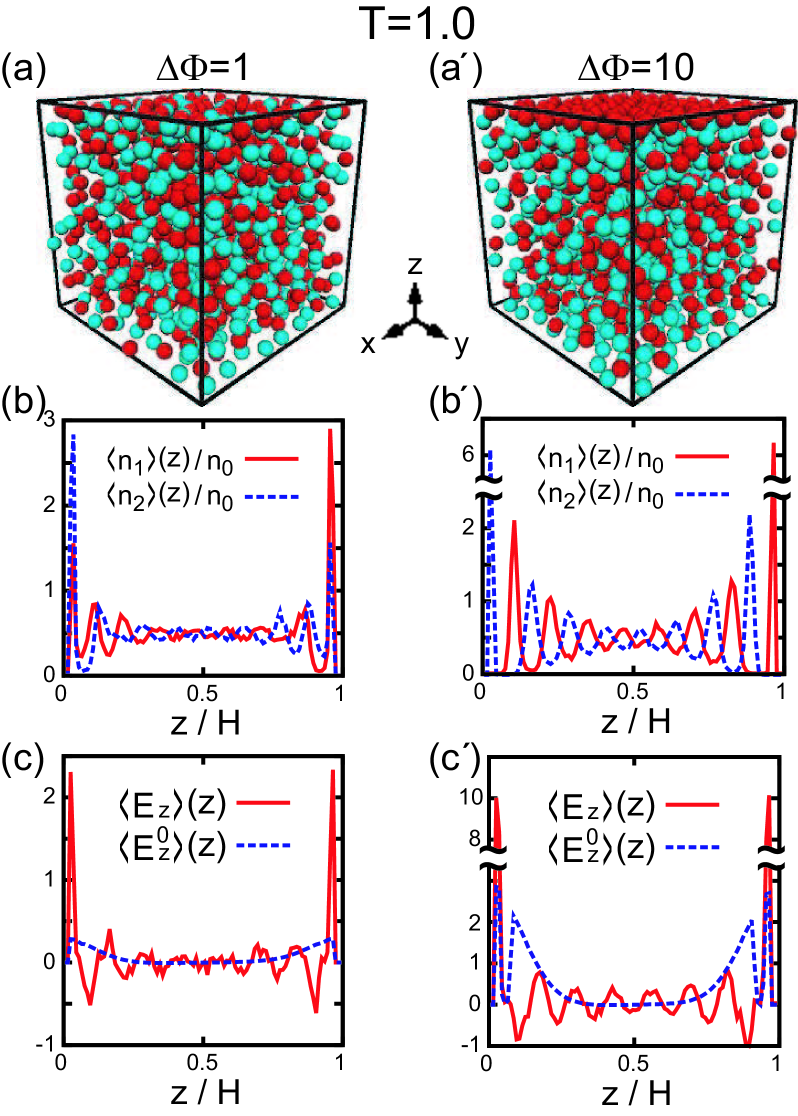
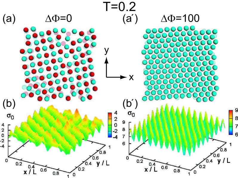
II.3.2 Charged particles at $T=1$: Screening effect

In Figs.2 and 3, we show simulation results in liquid at $T=1$ for $\Delta\Phi=1$ and $10$. In Fig.2(a)-(a^′), snapshots of the particles are given. In Fig.2(b)-(b^′), cross-sectional densities $\langle{n_{1}}\rangle(z)$ and $\langle{n_{2}}\rangle(z)$ are displayed, which show accumulation of the negative (positive) charges near the wall at $z=0$ ($z=H$). They are defined as follows. Let $\Delta N_{\alpha}(z)=\sum_{j\in\alpha}{\theta(z_{j}-z)\theta(z+\Delta z-z_{j})}$ be the particle numbers in layers $[z,z+\Delta z]$ ($z=n\Delta z$ with $n=0,1,\cdots)$ for the two species $\alpha=1,2$. The $\theta(u)$ is the step function being 1 for $u>0$ and 0 for $u\leq 0$. In this subsection, we set $\Delta z=H/100=0.12$, which is much smaller than the particle size. The laterally averaged densities for the two species are given by

$$\langle{n_{\alpha}}\rangle(z)=\langle{\Delta N_{\alpha}(z,t)}\rangle/L^{2}\Delta z.$$ (2.41)

Hereafter, $\langle{\cdots}\rangle$ represents the average over a time interval with width $10^{3}$.

In Fig.2(c)-(c^′), we display the laterally averaged (local) electric field along the $z$ axis calculated from

$$\langle{E_{z}}\rangle(z)=\sum_{j}\langle{E_{zj}\frac{\theta(z_{j}-z)\theta(z+\Delta z-z_{j})}{\Delta N(z)}}\rangle,$$ (2.42)

where $q_{j}E_{zj}=-\partial U_{\rm m}/\partial z_{j}$ and $\Delta N(z)=\Delta N_{1}(z)+\Delta N_{2}(z)$. We can see that $\langle{E_{z}}\rangle(z)$ exhibits sharp peaks near the walls but tends to zero in the interior. This screening is achieved only by one or two layers of the accumulated charges. In the same manner, replacing $E_{zj}$ in Eq.(2.42) by $E_{zj}^{s}$, $E_{zj}^{\ell}$, and $E_{j}^{0}$ in Eq.(2.33), we may define the lateral averages $\langle{E^{s}_{z}}\rangle(z)$, $\langle{E_{z}^{\ell}}\rangle(z)$, and $\langle{E^{0}}\rangle(z)$, respectively. For the examples in this subsection, we find $\langle{E_{z}^{\ell}}\rangle(z)\cong 0$ (less than 0.01) so that

$$\langle{E_{z}}\rangle(z)\cong\langle{E_{z}^{s}}\rangle(z)+\langle{E^{0}_{z}}\rangle(z).$$ (2.43)

In Fig.2(c)-(c^′), $\langle{E^{0}}\rangle(z)$ more smoothly varies than $\langle{E_{z}}\rangle(z)$ and tends to zero far from the walls, while $\langle{E_{z}^{s}}\rangle(z)$ exhibits sharp peaks near the walls and oscillates around zero far from the walls.

Figure 4: (Color online) Simulation results of charged particles in crystal at $T=0.2$. Cations (in red) and anions (in blue) for $\Delta\Phi=1$ in (a) and $100$ in (a^′). Normalized lateral density averages $\langle{n_{1}}\rangle(z)/n_{0}$ and $\langle{n_{2}}\rangle(z)/n_{0}$ are in (b) and (b^′). Lateral average $\langle{E_{z}}\rangle(z)$ are in (c) and (c^′). For $\Delta\Phi=0$, both cations and anions are somewhat denser in the first layer with larger $\langle{E_{z}}\rangle$ with a negative $\langle{E_{z}}\rangle$ in the second layer. For $\Delta\Phi=100$, anions are closely packed in the first layer, while their lateral density gradually decreases from the second layer. These ordered configurations are nearly stationary.

Figure 5: (Color online) Particle configuration in the first layer $0<z<1$ (in red or blue) and in the second layer $1<z<2$ (in lighter colors) for $\Delta\Phi=0$ in (a) and $100$ in (a^′). Surface charge density $\sigma_{0}(x,y)$ at $z=0$ for $\Delta\Phi=0$ in (b) and $100$ in (b^′) in units of $(\epsilon/\sigma^{3})^{1/2}$. Data are common to those in (a) and (a^′) of Fig.4. For $\Delta\Phi=0$, a square lattice (with defects) appears from the first layer. For $\Delta\Phi=100$, anions form a hexagonal lattice in the first layer, but are in a transition state in the second layer.

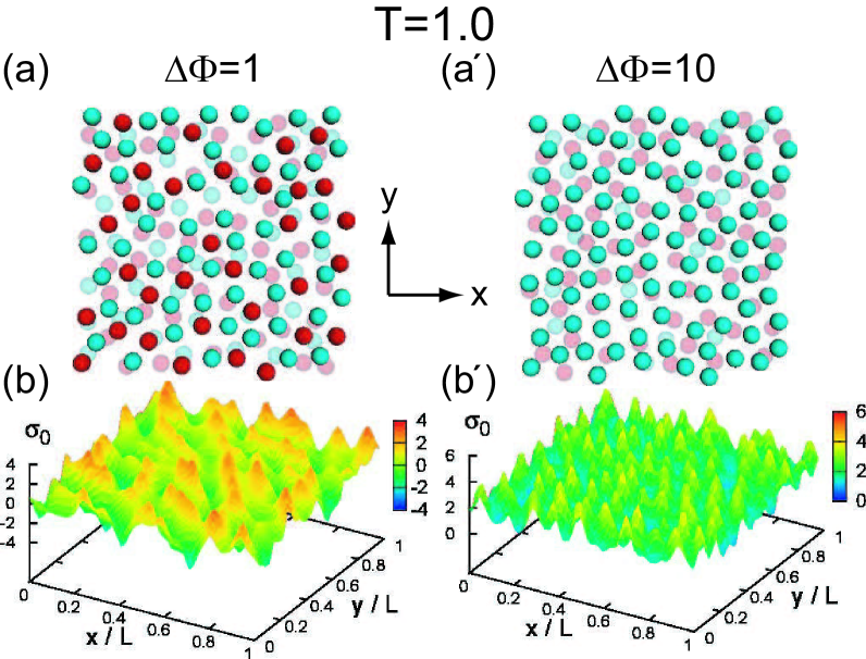
In Fig.3, we show snapshots of the particles in the two layers $0<z<1$ and $1<z<2$. For $\Delta\Phi=1$, cations and anions are both attracted to the wall due to the image interaction. For $\Delta\Phi=10$, only anions are attached in the first layer, but cations are richer in the second layer.

We divide Eq.(2.31) by $qL^{2}$ to obtain

$$Q_{0}/qL^{2}=E_{a}/4\pi q+\sum_{j}q_{j}z_{j}/qHL^{2},$$ (2.44)

where the second term is the areal density of excess cations at the top (with $z_{j}\cong H$) and is larger than the first term for strong screening commentS . The data in Figs.2(a)-(a^′) give $(E_{a}/4\pi q,\sum_{j}q_{j}z_{j}/qHL^{2})=(0.0013,0.106)$ for $\Delta\Phi=1$ and $(0.0013,0.426)$ for $\Delta\Phi=10$.

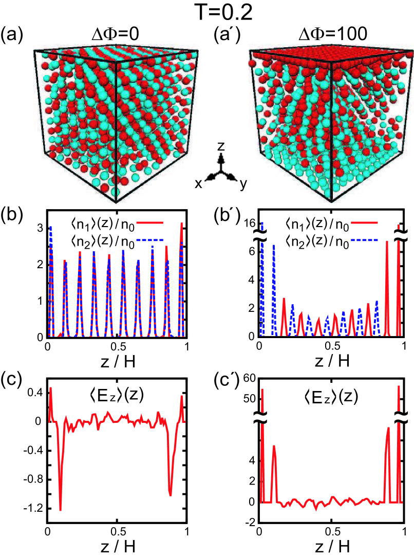
II.3.3 Charged particles at $T=0.2$: Ionic crystals

In Figs.4 and 5, we show simulation results in crystal at $T=0.2$. For $\Delta\Phi=0$ the cations and anions form a square lattice, as is well known for salts such as NaCl, from the first layer. However, for $\Delta\Phi=100$, we can see a hexagonal structure in the first layer $0<z<1$ and a square lattice for $z>2$, where the structure changes over in the second layer $1<z<2$. In this case, the first layer is composed of anions only and the second layer is anion-rich, as can also be seen in Fig.4(b^′). In the lower plates of Fig.5, the surface charge density $\sigma_{0}(x,y)$ varies nearly in one direction as a result of the complex charge distributions in the first few layers.

In addition, we examine Eq.(2.44). From the data in Figs.4(a)-(a^′) we have $(E_{a}/4\pi q,\sum_{j}q_{j}z_{j}/qHL^{2})=(0,0.024)$ for $\Delta\Phi=1$ and $(0.132,1.31)$ for $\Delta\Phi=100$. In the second example, the first layers next to the walls are nearly closely packed with cations or anions, as can be seen in Fig.5(a^′).

III Polar particles

In this section, we consider $N$ polar particles at positions ${\mbox{\boldmath$r$}}_{j}$ and with dipole moments ${\mbox{\boldmath$\mu$}}_{j}$. The derivatives of the electrostatic energy $U$ give the electrostatic force ${\mbox{\boldmath$F$}}_{i}^{e}$ and the electric field ${\mbox{\boldmath$E$}}_{i}$ on dipole $i$ as

$${\mbox{\boldmath$F$}}_{i}^{e}=-\frac{\partial}{\partial{\mbox{\boldmath$r$}}_{i}}U,\quad{\mbox{\boldmath$E$}}_{i}=-\frac{\partial}{\partial{\mbox{\boldmath$\mu$}}_{i}}U,$$ (3.1)

which are used in the equations of motions. There can also be neutral and charged particles.

III.1 Ewald method for dipoles in the periodic boundary condition

We first consider the electrostatic energy in the periodic boundary condition Allen ; Frenkel ; Leeuwreview , which is written as $U_{\rm p}^{\rm d}$. Here, there is no applied electric field. In Eq.(2.3) we replace $q_{i}$ by ${\mbox{\boldmath$\mu$}}_{i}\cdot\nabla_{j}$, where $\nabla_{i}=\partial/\partial{\mbox{\boldmath$r$}}_{i}$. Then, we obtain

$$U_{\rm p}^{\rm d}=\frac{1}{2}\sum_{\mbox{\boldmath$m$}}{\sum_{i,j}}^{\prime}({\mbox{\boldmath$\mu$}}_{i}\cdot\nabla_{i})({\mbox{\boldmath$\mu$}}_{j}\cdot\nabla_{j})\frac{1}{|{\mbox{\boldmath$r$}}_{ij}+L{\mbox{\boldmath$m$}}|}.$$ (3.2)

From Eq.(2.7) the Ewald representation is given by

$$U_{\rm p}^{\rm d}=\frac{1}{2}\sum_{\mbox{\boldmath$m$}}{\sum_{i,j}}^{\prime}{\mbox{\boldmath$\mu$}}_{i}\cdot{\stackrel{{\scriptstyle\leftrightarrow}}{{w}}}_{s}({|{\mbox{\boldmath$r$}}_{ij}+L{\mbox{\boldmath$n$}}|})\cdot{\mbox{\boldmath$\mu$}}_{j}$$

$$+\frac{1}{2L^{3}}{\sum_{{\mbox{\boldmath$k$}}}}^{\prime}\sum_{i,j}({\mbox{\boldmath$k$}}\cdot{\mbox{\boldmath$\mu$}}_{i})({\mbox{\boldmath$k$}}\cdot{\mbox{\boldmath$\mu$}}_{j})\Psi_{\ell}(k)e^{{\rm i}{\mbox{\boldmath$k$}}\cdot{\mbox{\boldmath$r$}}_{ij}}$$

$$-\sum_{i}\frac{2\gamma^{3}}{3\sqrt{\pi}}|{\mbox{\boldmath$\mu$}_{i}}|^{2}+\frac{2\pi}{3L^{3}}\bigg{|}\sum_{j}{\mbox{\boldmath$\mu$}}_{j}\bigg{|}^{2}.$$ (3.3)

In the first term, we introduce the tensor ${\stackrel{{\scriptstyle\leftrightarrow}}{{w}}}_{s}({\mbox{\boldmath$r$}})$ by

$$\stackrel{{\scriptstyle\leftrightarrow}}{{w}}_{s}({\mbox{\boldmath$r$}})=-\nabla\nabla\psi_{s}(r)=B(r)\stackrel{{\scriptstyle\leftrightarrow}}{{I}}-C(r)\frac{1}{r^{2}}{\mbox{\boldmath$r$}}{\mbox{\boldmath$r$}},$$ (3.4)

where $\stackrel{{\scriptstyle\leftrightarrow}}{{I}}$ is the unit tensor and

$$B(r)=\psi_{s}(r)/r^{2}+2\pi\varphi_{3}(r)/\gamma^{2}r^{2},$$

$$C(r)=3B(r)+4\pi\varphi_{3}(r),$$ (3.5)

with $\varphi_{3}(r)=\varphi(x)\varphi(y)\varphi(z)$ (see Eq.(2.5)). The third term in Eq.(3.3) is the counterpart of the second term in Eq.(2.7) following from the small-$r$ expansion (2.6).

III.2 Ewald method for dipoles between metallic plates under applied electric field

We consider $N$ dipoles between metallic plates in applied electric field $E_{a}$. The electrostatic potential $\Phi$ is written as Eq.(2.12). For each dipole ${\mbox{\boldmath$\mu$}}_{i}=(\mu_{xi},\mu_{yi},\mu_{zi})$ at ${\mbox{\boldmath$r$}}_{i}=(x_{j},y_{j},z_{j})$, there arise S-image dipoles at $(x_{i},y_{i},z_{i}-2Hn)$ ($n\neq 0$) with the same moment ${\mbox{\boldmath$\mu$}}_{i}$ and O-image dipoles at $(x_{i},y_{i},-z_{i}-2Hn)$ with the moment,

$$\bar{\mbox{\boldmath$\mu$}}_{i}=(-\mu_{xi},-\mu_{yi},\mu_{zi}).$$ (3.6)

See Fig.1 for these images. If a dipole at ${\mbox{\boldmath$r$}}_{i}$ approaches the bottom wall, its image at ${\bar{\mbox{\boldmath$r$}}}_{i}$ yields the dipolar electric field $-\partial v_{\rm I}^{\rm d}/\partial{\mbox{\boldmath$\mu$}}_{i}=-(2z_{i})^{-3}(\bar{{\mbox{\boldmath$\mu$}}}_{i}-3\bar{\mu_{zi}}{\mbox{\boldmath$e$}}_{z})$ at ${\mbox{\boldmath$r$}}_{i}$. Thus the interaction energy from this closest image is written as

$$v_{\rm I}^{\rm d}(z_{i},\theta_{i})=[{\mbox{\boldmath$\mu$}}_{i}\cdot{\bar{\mbox{\boldmath$\mu$}}}_{i}-3\mu_{zi}\bar{\mu}_{zi}]/2(2z_{i})^{3}$$

$$=-|{\mbox{\boldmath$\mu$}}_{i}|^{2}(1+\cos^{2}\theta_{i})/16z_{i}^{3},$$ (3.7)

where $\cos\theta_{i}=\mu_{zi}/|{\mbox{\boldmath$\mu$}}_{i}|$ with $\theta_{i}$ being the angle of ${\mbox{\boldmath$\mu$}}_{i}$ with respect to the $z$ axis. This interaction energy is negative and grows for small $z_{i}$. In the vicinity of the wall, where $|v_{\rm I}^{\rm d}|\gg k_{B}T$ holds, dipoles are attracted to the walls and are oriented in the parallel direction ($\theta_{i}=0$) or in the antiparallel direction ($\theta_{i}=\pi$) with respect to the $z$ axis.

From the formulae in the previous section, we obtain the counterparts by replacing $q_{j}$ by ${\mbox{\boldmath$\mu$}}_{j}\cdot\nabla_{j}$ for S-images and $-q_{j}$ by ${\bar{\mbox{\boldmath$\mu$}}}_{j}\cdot\nabla_{j}$ for O-images, where $\nabla_{j}=\partial/\partial{\mbox{\boldmath$r$}}_{j}$. From Eq.(2.21) the excess potential $\phi({\mbox{\boldmath$r$}})$ for ${\mbox{\boldmath$r$}}\neq{\mbox{\boldmath$r$}}_{j}$ is obtained in the following superposition,

$$\phi=\sum_{{\mbox{\boldmath$m$}}}{\sum_{j}}\nabla_{j}\cdot\bigg{[}\frac{{\mbox{\boldmath$\mu$}}_{j}}{|{\mbox{\boldmath$r$}}-{\mbox{\boldmath$r$}}_{j}+{\mbox{\boldmath$h$}}|}+\frac{{\bar{\mbox{\boldmath$\mu$}}}_{j}}{|{\mbox{\boldmath$r$}}-{\bar{\mbox{\boldmath$r$}}}_{j}+{\mbox{\boldmath$h$}}|}\bigg{]},$$ (3.8)

which surely vanishes at $z=0$ and $H$. The total electrostatic energy in the fixed-potential condition is written as $U_{\rm m}^{\rm d}$. From Eq.(2.23), we find

$$U_{\rm m}^{\rm d}=\frac{1}{2}\sum_{\mbox{\boldmath$m$}}\bigg{[}{\sum_{i,j}}^{\prime}({\mbox{\boldmath$\mu$}}_{i}\cdot\nabla_{i})({\mbox{\boldmath$\mu$}}_{j}\cdot\nabla_{j})\frac{1}{|{\mbox{\boldmath$r$}}_{ij}+{\mbox{\boldmath$h$}}|}$$

$$+{\sum_{i,j}}({{\mbox{\boldmath$\mu$}}}_{i}\cdot\nabla_{i})({\bar{\mbox{\boldmath$\mu$}}}_{j}\cdot\nabla_{j})\frac{1}{|{\bar{\mbox{\boldmath$r$}}}_{ij}+{\mbox{\boldmath$h$}}|}\bigg{]}-E_{a}\sum_{i}\mu_{iz},$$ (3.9)

where the self-interaction terms are removed in $\sum_{i,j}^{\prime}$ and $h$ is given by Eq.(2.22). The direct image interaction energy in Eq.(3.7) is included in the above expression. From Eq.(3.1) the differential form of $U_{\rm m}^{\rm d}$ is given by

$$dU_{\rm m}^{\rm d}=-\sum_{i}({\mbox{\boldmath$F$}}_{i}^{e}\cdot d{\mbox{\boldmath$r$}}_{i}+{\mbox{\boldmath$E$}}_{i}\cdot d{\mbox{\boldmath$\mu$}}_{i})-\sum_{i}\mu_{zi}dE_{a}.$$ (3.10)

The Ewald representation of $U_{\rm m}^{\rm d}$ may be written as Klapp

$$U_{\rm m}^{\rm d} = \frac{1}{2}\sum_{\mbox{\boldmath$m$}}{\sum_{i,j}}^{\prime}{\mbox{\boldmath$\mu$}}_{i}\cdot{\stackrel{{\scriptstyle\leftrightarrow}}{{w}}}_{s}({|{\mbox{\boldmath$r$}}_{ij}+{\mbox{\boldmath$h$}}|})\cdot{{\mbox{\boldmath$\mu$}}}_{j}$$ (3.11)

$$+\frac{1}{2}\sum_{\mbox{\boldmath$m$}}{\sum_{i,j}}{\mbox{\boldmath$\mu$}}_{i}\cdot{\stackrel{{\scriptstyle\leftrightarrow}}{{w}}}_{s}({|{\bar{\mbox{\boldmath$r$}}}_{ij}+{\mbox{\boldmath$h$}}|})\cdot{\bar{\mbox{\boldmath$\mu$}}}_{j}-\sum_{i}\frac{2\gamma^{3}}{3\sqrt{\pi}}|{\mbox{\boldmath$\mu$}_{i}}|^{2}$$

$$+\frac{1}{HL^{2}}{\sum_{{\mbox{\boldmath$\nu$}}_{\perp}\neq{\mbox{\boldmath$0$}}}}\sum_{i,j}\frac{\Psi_{\ell}(k)}{4}({\mbox{\boldmath$k$}}\cdot{\mbox{\boldmath$\mu$}}_{i}){\mbox{\boldmath$k$}}\cdot(e^{{\rm i}{\mbox{\boldmath$k$}}\cdot{\mbox{\boldmath$r$}}_{ij}}{\mbox{\boldmath$\mu$}}_{j}+e^{{\rm i}{\mbox{\boldmath$k$}}\cdot{\bar{\mbox{\boldmath$r$}}}_{ij}}{\bar{\mbox{\boldmath$\mu$}}}_{j})$$

$$+V_{\rm m}^{\rm d}-E_{a}\sum_{i}\mu_{zi}.$$

The first and second terms represent the short-range part with $\stackrel{{\scriptstyle\leftrightarrow}}{{w}}_{s}$ given in Eq.(3.4). The third term has appeared in Eq.(3.3). In the fourth long-range term, the summation is over ${\mbox{\boldmath$\nu$}}=(\nu_{x},\nu_{y},\nu_{z})$ with ${\mbox{\boldmath$\nu$}}_{\perp}=(\nu_{x},\nu_{y})\neq{\mbox{\boldmath$0$}}$ and $k$ is given by Eq.(2.27). The fifth term $V_{\rm m}^{\rm d}$ arises from the contributions with $k_{x}=k_{y}=0$. From Eqs.(2.26), (2.28), and (C4), we find

$$V_{\rm m}^{\rm d}=\frac{2\pi}{L^{2}}\sum_{ij}\mu_{zi}\mu_{zj}\bigg{[}\hat{\varphi}(z_{i}-z_{j})+\hat{\varphi}(z_{i}+z_{j})-\frac{1}{H}\bigg{]}$$

$$\hskip 17.07164pt=\frac{4\pi}{HL^{2}}\sum_{n\geq 1}e^{-(\pi n/2\gamma H)^{2}}K_{n}^{2},$$ (3.12)

where $K_{n}$ depends on $z_{1},z_{2},\cdots$ as

$$K_{n}=\sum_{j}\mu_{zj}\cos(\frac{\pi nz_{j}}{H}).$$ (3.13)

The electric field ${\mbox{\boldmath$E$}}_{i}$ on dipole $i$ can be calculated from Eq.(3.11). That is, the contribution from the first and second terms, that from the third and fourth terms, and that from the fifth and sixth terms are written as ${\mbox{\boldmath$E$}}_{i}^{\rm ds}$, ${\mbox{\boldmath$E$}}_{i}^{{\rm d}\ell}$, and $E_{i}^{{\rm d}0}{\mbox{\boldmath$e$}}_{z}$, respectively. Then,

$${\mbox{\boldmath$E$}}_{i}={\mbox{\boldmath$E$}}_{i}^{\rm ds}+{\mbox{\boldmath$E$}}_{i}^{{\rm d}\ell}+{E}_{i}^{{\rm d}0}{\mbox{\boldmath$e$}}_{z}.$$ (3.14)

From Eq.(3.12) ${E}_{i}^{{\rm d}0}$ is expressed as

$$E_{i}^{d0}=E_{a}-\frac{4\pi}{L^{2}}\sum_{j}\mu_{zj}\bigg{[}{\hat{\varphi}}(z_{i}-z_{j})+{\hat{\varphi}}(z_{i}+z_{j})-\frac{1}{H}\bigg{]}$$

$$=E_{a}-\frac{8\pi}{HL^{2}}\sum_{n\geq 1}e^{-({\pi n}/{2\gamma H})^{2}}K_{n}\cos(\frac{\pi nz_{i}}{H}).$$ (3.15)

In the first line, if the particles $j$ ($\neq i$) are randomly distributed in the cell, the second term vanishes, and the self term with $j=i$ is of order $\mu_{zi}\gamma/L^{2}$. Thus, if the boundary disturbances do not extend into the interior in a thick and wide cell, we have $E_{i}^{d0}\cong E_{a}$ (see Table 1 below). The first line of Eq.(3.15) is consistent with Eq.(D5) in Appendix D.

By replacing $q_{j}$ by ${\mbox{\boldmath$\mu$}}_{j}\cdot\nabla_{j}$ in Eq.(2.30), we obtain the surface charge densities, $\sigma_{0}(x,y)$ at $z=0$ and $\sigma_{H}(x,y)$ at $z=H$, in the 2D Fourier expansions,

$$\sigma_{0}=\frac{{E_{a}}}{4\pi}-\frac{1}{L^{2}}\sum_{{\mbox{\boldmath$\nu$}}_{\perp}}\sum_{j}{\mbox{\boldmath$\mu$}}_{j}\cdot\nabla_{j}\frac{\sinh(kH-kz_{j})}{\sinh(kH)}e^{{\rm i}{\mbox{\boldmath$k$}}\cdot({\mbox{\boldmath$r$}}-{\mbox{\boldmath$r$}}_{j})},$$

$$\sigma_{H}=-\frac{{E_{a}}}{4\pi}-\frac{1}{L^{2}}\sum_{{\mbox{\boldmath$\nu$}}_{\perp}}\sum_{j}{\mbox{\boldmath$\mu$}}_{j}\cdot\nabla_{j}\frac{\sinh(kz_{j})}{\sinh(kH)}e^{{\rm i}{\mbox{\boldmath$k$}}\cdot({\mbox{\boldmath$r$}}-{\mbox{\boldmath$r$}}_{j})},$$

where ${\mbox{\boldmath$\nu$}}_{\perp}=(\nu_{x},\nu_{y})$ and ${\mbox{\boldmath$k$}}=(2\pi\nu_{x}/L,2\pi\nu_{y}/L,0)$. Integrating $\sigma_{0}$ and $\sigma_{H}$ in the planar region $0<x,y<L$ yields the total electric charges on the metallic surfaces,

$$Q_{0}=-Q_{H}=\frac{1}{4\pi}L^{2}E_{a}+\frac{1}{H}\sum_{j}\mu_{zj}.$$ (3.17)

See Eq.(D6) for the counterpart in the continuum theory.

III.3 Numerical example for dipoles between metallic plates under applied electric field

III.3.1 Model and method

Next, we present results of molecular dynamics simulation of one-component spherical dipoles with number $N=1000$ between parallel metallic plates with $H=L$ at fixed potential difference $\Delta\Phi$.

As in Eq.(2.35), the total potential energy is given by

$$U_{\rm tot}=U_{\rm m}^{\rm d}+\sum_{i>j}v_{s}(r_{ij})+\sum_{i}v_{\rm w}(z_{i}),$$ (3.18)

where $U_{\rm m}^{\rm d}$ is given by Eq.(3.11), $v_{s}(r)$ by Eq.(2.36), and $v_{\rm w}(z)$ by Eq.(2.37). Hereafter, in terms of $\sigma$ and $\epsilon$ in $v_{s}(r)$, units of length, density, electrostatic potential, electric field, electric charge, dipole moment, and temperature are $\sigma$, $\sigma^{-3}$, $(\epsilon/\sigma)^{1/2}$, $(\epsilon/\sigma^{3})^{1/2}$, $(\epsilon\sigma)^{1/2}$, $(\epsilon\sigma^{3})^{1/2}$, and $\epsilon/k_{B}$, respectively. The average density $n_{0}=N/HL^{2}$ is chosen to be $0.19$, $0.38,$ and 0.57; then, $L=17.4,13.8$, and 12.0, respectively.

We cut off $v_{s}(r)$ and the short-range part of $U_{\rm m}^{\rm d}$ in Eq.(3.11) at $r=r_{\rm cut}^{s}=4$. In $U_{\rm m}^{\rm d}$, we set $\gamma=0.65$ and sum over $k$ in the region $k\leq k_{c}=18\pi/L$. Thus, in $E_{i}^{{\rm d}0}$ in Eq.(3.15), the terms up to $n=18$ are summed. In addition, we note that the simulation results are rather insensitive to the choice of $\gamma$. To confirm this, we also performed simulations for $\gamma=0.5$ and $1$ with $r_{\rm cut}^{s}=6$ for the case of $n_{0}=0.19$, $T=1.0$, and $E_{a}=0.058$. Then the numbers in the first line of Table 1 were changed only slightly with differences less than $5\%$.

The dipole moment has a fixed magnitude $\mu_{0}$ as

$${\mbox{\boldmath$\mu$}}_{i}=\mu_{0}{\mbox{\boldmath$n$}}_{i},$$ (3.19)

where ${\mbox{\boldmath$n$}}_{i}$ is the unit vector representing the direction of polarization. In this subsection, we set

$$\mu_{0}=|{\mbox{\boldmath$\mu$}}_{i}|=2(\epsilon\sigma^{3})^{1/2}.$$ (3.20)

Then our system is highly polarizable at high densities.

The total kinetic energy is assumed to be of the form,

$$K_{\rm tot}=\sum_{i}\frac{m}{2}|{\dot{\mbox{\boldmath$r$}}}_{i}|^{2}+\sum_{i}\frac{I_{1}}{2}|{\dot{\mbox{\boldmath$n$}}}_{i}|^{2},$$ (3.21)

where ${\dot{\mbox{\boldmath$r$}}}_{i}=d{\mbox{\boldmath$r$}}_{i}/dt$, ${\dot{\mbox{\boldmath$n$}}}_{i}=d{\mbox{\boldmath$n$}}_{i}/dt$, and $I_{1}$ is the moment of inertia. Regarding dipoles as spheres with diameter $\sigma$, we set $I_{1}=m\sigma^{2}/10$. The Newton equations of motions for ${\mbox{\boldmath$r$}}_{i}$ and ${\mbox{\boldmath$n$}}_{i}$ are written asEPL

$$m\frac{d^{2}}{dt^{2}}{{\mbox{\boldmath$r$}}}_{i}=-\frac{\partial{}}{\partial{{\mbox{\boldmath$r$}}_{i}}}U_{\rm tot},$$ (3.22)

$$I_{1}{\mbox{\boldmath$n$}}_{i}\times\frac{d^{2}}{dt^{2}}{{\mbox{\boldmath$n$}}}_{i}=-{\mbox{\boldmath$\mu$}}_{i}\times\frac{\partial{}}{\partial{{\mbox{\boldmath$\mu$}}_{i}}}U_{\rm tot},$$ (3.23)

where ${\mbox{\boldmath$n$}}_{i}\cdot{d^{2}{\mbox{\boldmath$n$}}_{i}/dt^{2}}=-|{\dot{\mbox{\boldmath$n$}}}_{i}|^{2}$ from ${\mbox{\boldmath$n$}}_{i}\cdot{\dot{\mbox{\boldmath$n$}}}_{i}=0$. The total energy $U_{\rm tot}+K_{\rm tot}$ is conserved in time. We integrated these equations in the NVE ensemble using the leap-frog method with the time step width being $0.002$, as in the previous section (see below Eq.(2.40)). The translational and rotational kinetic energies were kept at $3k_{B}T/2$ and $k_{B}T$, respectively, per particle.

III.3.2 Highly polarizable liquids

Figure 6: (Color online) Snapshots of spherical dipoles in liquid at $T=1$: (a) $n_{0}=0.19$ and $\Delta\Phi=1$, (b) $n_{0}=0.19$ and $\Delta\Phi=10$, (c) $n_{0}=0.38$ and $\Delta\Phi=1$, and (d) $n_{0}=0.38$ and $\Delta\Phi=10$. Colors represent the orientation of ${\mbox{\boldmath$\mu$}}_{i}$ as in Fig.7.

Figure 7: (Color online) Color maps of polarization direction ${\mbox{\boldmath$n$}}_{i}$ on a sphere surface: (a) Diagonally downward view, (b) diagonally upward view, (c) top view, and (d) bottom view. Spheres become white (gray) as they are parallel (antiparallel) to the applied field.

Figure 8: (Color online) Top: Dipole configurations in the two layers $0<z<1$ and $1<z<2$ for $\Delta\Phi=1$ (left) and $10$ (right), according to the color maps in Fig.7. Bottom: Surface charge density $\Delta\sigma_{0}(x,y)$ at $z=0$ for $\Delta\Phi=1$ and $10$ in units of $(\epsilon/\sigma^{3})^{1/2}$. Data are common to those in (a) and (a^′) of Fig.6.

Figure 9: (Color online) Simulation results of spherical dipoles for $n_{0}=0.38$ and $T=1$ in liquid, where $\Delta\Phi=1$ (left) and $10$ (right). Normalized lateral density average $\langle{n}\rangle(z)/n_{0}$ is in (b) and (b^′). Lateral average $\langle{E_{z}}\rangle(z)$ are in (c) and (c^′) and that $\langle{4\pi p_{z}}\rangle(z)$ are in (d) and (d^′). Here, $\Delta z=H/100$ (bold red lines) and $\Delta z=H/20$ (broken blue lines), where $\Delta z$ is the smoothing length.

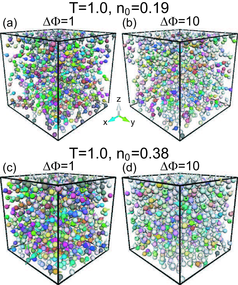
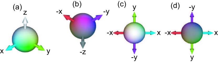
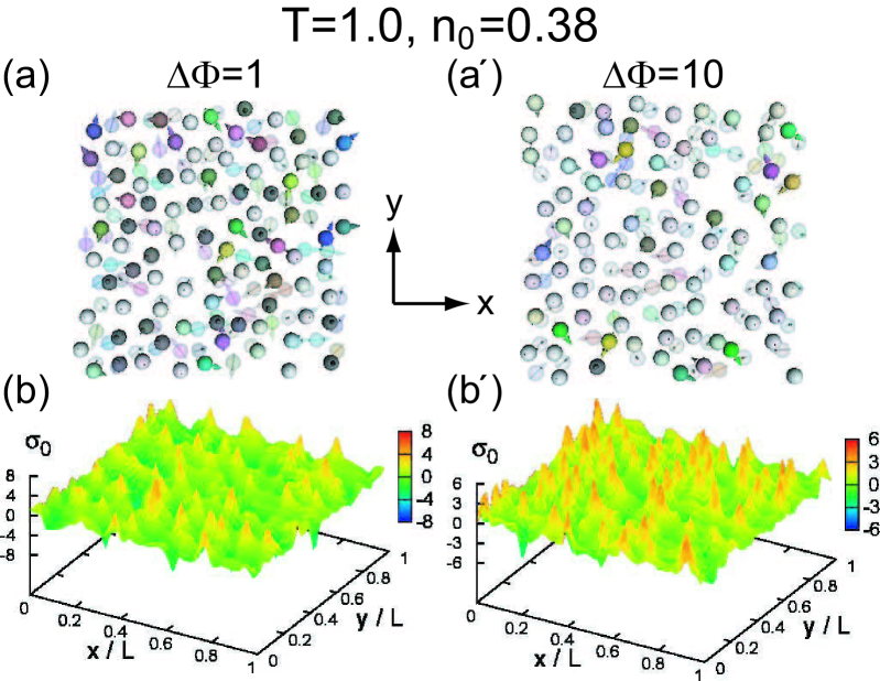
In Fig.6, we show snapshots of spherical dipoles for $n_{0}=0.19$ and $0.38$ in liquid at $T=1$ under $\Delta\Phi=1$ and 10. The colors of the spheres represent their polarization directions according to the color maps in Fig.7. We can see orientation enhancement with increasing $\Delta\Phi$. For $n_{0}=0.19$, chainlike associations are clearly visualized, whose lengths increase with increasing $\Delta\Phi$. For small $\Delta\Phi$ a large number of dimers appear.

In the top panels of Fig.8, we display particle configurations near the bottom wall in the two layers, $0<z<1$ and $1<z<2$, and the surface charge density $\sigma_{0}(x,y)$ in Eq.(3.16). In these cases, dipoles are accumulated on the walls and are oriented. For $\Delta\Phi=1$, the image interaction (3.7) is strong enough to induce alignment both in the parallel and antiparallel directions along the $z$ axis. For $\Delta\Phi=10$ those in the parallel direction increase. In the bottom panels of Fig.8, the surface charge density in Eq.(3.16) are written, which are highly heterogeneous and fluctuating in time.

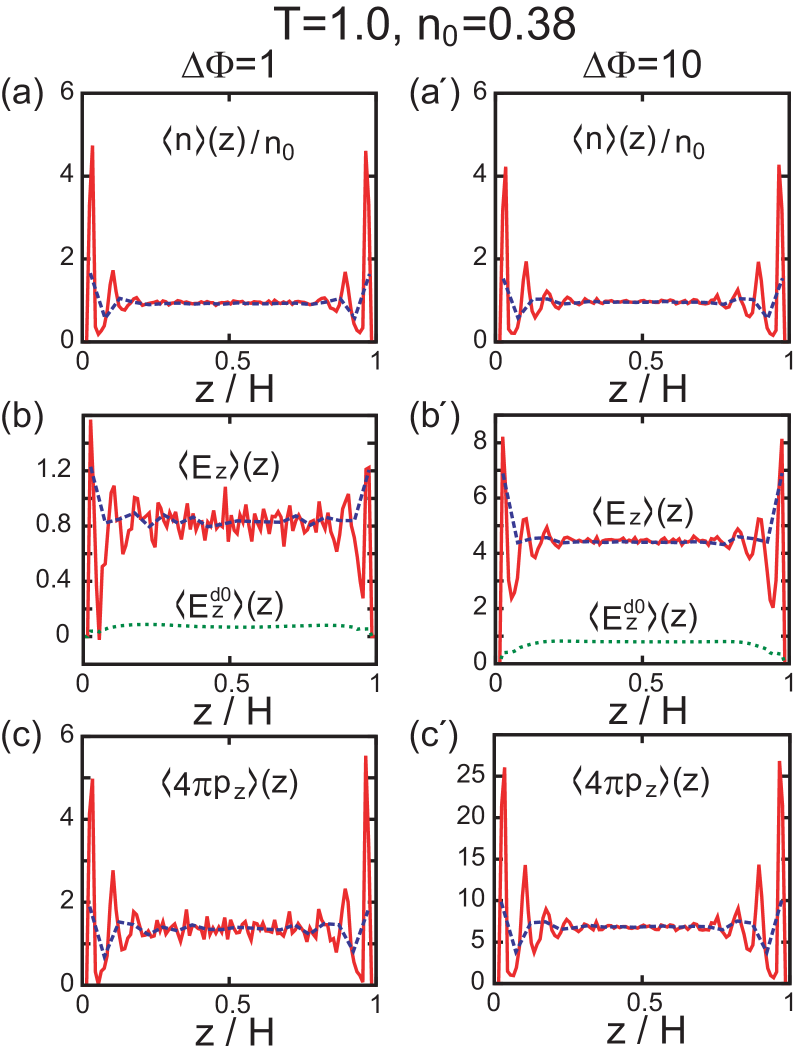
In Figs.9(a)-(a^′), we display the laterally averaged density $\langle{n}\rangle(z)$ defined as in Eq.(2.41), where we write two curves for $\Delta z=H/100=0.138$ and $H/20=0.69$. We recognize that the interior away from the walls is in a homogeneous, uniaxial equilibrium state under electric field for $H\gg 1$. In Table 1, the bulk density $\bar{n}$ in the interior is slightly smaller than $n_{0}$ because the dipoles are accumulated near the walls. We determined the interior (bulk) values from the lateral averages with $\Delta z=H/20$.

Table 1: Data for 1000 spherical dipoles in liquid at $T=1$ in a $L\times L\times H$ cell ($H=L$) under applied potential difference $\Delta\Phi=HE_{a}=1$ and 10 for three densities $n_{0}=0.19$, $0.38$, and $0.57$. Here, $\bar{n}$, ${\bar{\mu}}_{z}$, and ${\bar{p}}_{z}={\bar{n}}{\bar{\mu}}_{z}$ are bulk values in the interior. Also given are bulk values of $\langle{E^{{\rm d}0}}\rangle(z)$ and $\langle{E_{z}}\rangle(z)$, dielectric constant $\varepsilon_{\rm e}$ in Eq.(3.29), local field factor $\gamma_{\ell}$ in Eq.(3.30), polarizability $\alpha_{\rm e}={\bar{\mu}}_{z}/\langle{E_{z}}\rangle$.

$n_{0}$	$E_{a}$	$Q_{0}$	$\langle{E^{{\rm d}0}}\rangle$	${\bar{n}}/{n_{0}}$	${\bar{\mu}}_{z}$	$4\pi{\bar{p}}_{z}$	$\langle{E_{z}}\rangle$	$\varepsilon_{\rm e}$	$\gamma_{\ell}$	$\alpha_{\rm e}$
0.19	0.058	11.6	0.060	0.88	0.18	0.37	0.42	7.4	0.97	0.43
0.19	0.58	78.5	0.65	0.91	1.20	2.62	2.88	5.5	0.88	0.42
0.38	0.073	23.0	0.069	0.95	0.30	1.36	0.82	19.6	0.55	0.37
0.38	0.73	115	0.80	0.97	1.46	6.81	4.45	10.3	0.55	0.33
0.57	0.083	40.5	0.069	0.97	0.48	3.29	1.55	40.6	0.45	0.31
0.57	0.83	143	0.95	0.98	1.62	11.36	5.89	14.7	0.45	0.26

Using the decomposition (3.14) of the local field ${\mbox{\boldmath$E$}}_{i}$, we define the laterally averaged electric fields $\langle{E_{z}}\rangle(z)$, $\langle{E_{z}^{\rm ds}}\rangle(z)$, $\langle{E_{z}^{{\rm d}\ell}}\rangle(z)$, and $\langle{E^{{\rm d}0}}\rangle(z)$ as in Eq.(2.42). Hereafter, $\langle{\cdots}\rangle$ represents the average over a long time interval with width $10^{3}$. Along the $z$ axis we thus have

$$\langle{E_{z}}\rangle(z)=\langle{E_{z}^{\rm ds}}\rangle(z)+\langle{E_{z}^{{\rm d}\ell}}\rangle(z)+\langle{E^{{\rm d}0}}\rangle(z).$$ (3.24)

If the boundary layers are much thinner than $H$, we have $\langle{E^{{\rm d}0}}\rangle(z)\cong E_{a}$ in the interior (see the sentences below Eq.(3.15)). For the examples in Table 1, we can indeed see $\langle{E^{{\rm d}0}}\rangle\cong E_{a}$. We also find that $\langle{E_{z}^{{\rm d}\ell}}\rangle(z)$ is of the same order as $E_{a}$ ratio . In the bulk region of our examples, the short-range contribution $\langle{E_{z}^{\rm ds}}\rangle(z)$ is thus dominant in the right hand side of Eq.(3.24), typically being about $90\%$ of $\langle{E_{z}}\rangle$, so that

$$\langle{E_{z}}\rangle\cong\langle{E_{z}^{\rm ds}}\rangle.$$ (3.25)

We also define the lateral average of the polarization,

$$\langle{p_{z}}\rangle(z)=\sum_{j}\langle{\mu_{zj}\frac{\theta(z_{j}-z)\theta(z+\Delta z-z_{j})}{L^{2}\Delta z}}\rangle.$$ (3.26)

We plot $\langle{E_{z}}\rangle(z)$ in Fig.9(b)-(b^′) and $\langle{p_{z}}\rangle(z)$ in Fig.9(c)-(c^′) for $\Delta z=H/100$ and $H/20$, where the curves are more smooth for larger $\Delta z$. In the interior, they assume the bulk average values with small fluctuations. In Table 1, we give the average bulk values of $\langle{E_{z}}\rangle$, $\langle{E^{0}}\rangle(z)$, and $\langle{4\pi E_{z}}\rangle(z)$ at $T=1$ for three densities $n_{0}=0.19,0.38$, and 0.57 under $\Delta\Phi=1$ and 10.

In terms of the polarization variable,

$$\hat{\mbox{\boldmath$p$}}({\mbox{\boldmath$r$}})=\sum_{i}{\mbox{\boldmath$\mu$}}_{i}\delta({\mbox{\boldmath$r$}}_{i}-{\mbox{\boldmath$r$}}),$$ (3.27)

we have $\langle{p_{z}}\rangle(z)=\int_{0}^{L}dx\int_{0}^{L}dy\int_{z}^{z+{\Delta z}}dz{\hat{p}}_{z}({\mbox{\boldmath$r$}})/L^{2}\Delta z$. Averaging over the particles in the interior and over a long time yields the bulk average polarization,

$${\bar{p}}_{z}=\langle{\hat{p}_{z}}\rangle=\bar{n}{\bar{\mu}}_{z},$$ (3.28)

where ${\bar{\mu}}_{z}$ is the average of $\mu_{zi}$ in the interior. We define the effective dielectric constant by

$$\varepsilon_{\rm e}=1+4\pi{\bar{p}}_{z}/E_{a}.$$ (3.29)

In Table 1, $\varepsilon_{\rm e}$ is much larger than unity, increasing with increasing $n_{0}$ and decreasing with increasing $E_{a}$. For $\Delta\Phi=10$, ${\bar{\mu}}_{z}$ approaches its maximum $\mu_{0}=2$, where the system is in the nonlinear response regime. In addition, for $n_{0}=0.57$ and $\Delta\Phi=1$, $\varepsilon_{\rm e}$ is given by a large value of 40. With lowering $T$ at this density, we find occurrence of a ferroelectric phase transition around $T\cong 0.5$, on which we will report shortly.

Furthermore, since ${\mbox{\boldmath$E$}}_{i}$ is the local electric field, its lateral average $\langle{E_{z}}\rangle$ along the $z$ axis is related to the applied electric field $E_{a}$ and the local polarization ${\bar{p}}_{z}$ by

$$\langle{E_{z}}\rangle=E_{a}+4\pi\gamma_{\ell}{\bar{p}}_{z},$$ (3.30)

in the bulk region. The second term represents the Lorentz field with $\gamma_{\ell}$ being the local field factorOnsager ; Kirk ; local . The classical value of $\gamma_{\ell}$ is $1/3$. However, in Table 1, $\gamma_{\ell}$ considerably exceeds $1/3$. It increases with decreasing $n_{0}$ but is rather insensitive to $E_{a}$. We may also introduce the polarizability $\alpha_{\rm e}={\bar{\mu}}_{z}/\langle{E_{z}}\rangle$. Then, $\varepsilon_{\rm e}$ satisfies

$$\frac{{\varepsilon_{\rm e}}-1}{{1+\gamma_{\ell}(\varepsilon_{\rm e}-1)}}=4\pi{\bar{n}}\alpha_{\rm e},$$ (3.31)

which nicely holds in Table 1. The Clausius-Mossotti formula follows for $\gamma_{\ell}=1/3$. Here, we should suppose a thick cell ($H\gg 1$) to avoid the boundary effect in the relations (3.29) and (3.30), though our system size is still not large enough.

In our case, the classical local field relation breaks down because of strong pair correlations along the $z$ axis. To explain this, we assume a large homogeneous interior region in liquid for large $H$ and $L$. There, we define the pair correlation functions $g(r,\theta)$ and $g_{\rm p}(r,\theta)$ by

$$\langle{\hat{n}({\mbox{\boldmath$r$}_{0}})\hat{n}({\mbox{\boldmath$r$}_{0}}+{\mbox{\boldmath$r$}})}\rangle={\bar{n}}\delta({\mbox{\boldmath$r$}})+{\bar{n}}^{2}g(r,\theta),$$ (3.32)

$$\langle{\hat{n}({\mbox{\boldmath$r$}_{0}})\hat{{p}}_{z}({\mbox{\boldmath$r$}_{0}}+{\mbox{\boldmath$r$}})}\rangle={\bar{n}}\bar{{p}}_{z}\delta({\mbox{\boldmath$r$}})+{\bar{n}}{g}_{\rm p}(r,\theta),$$ (3.33)

where $\hat{n}({\mbox{\boldmath$r$}})=\sum_{i}\delta({\mbox{\boldmath$r$}}_{i}-{\mbox{\boldmath$r$}}_{0})$ is the density variable and $\hat{\mbox{\boldmath$p$}}({\mbox{\boldmath$r$}})$ is defined in Eq.(3.27). These relations are independent of ${\mbox{\boldmath$r$}}_{0}$ from the translational invariance. The $g(r,\theta)$ and $g_{\rm p}(r,\theta)$ depend only on $r$ and $\theta=\cos^{-1}(z/r)$ from the rotational invariance around the $z$ axis. For $r\gg 1$, we have $g(r,\theta)\to 1$ and $g_{\rm p}(r,\theta)\to{\bar{p}}_{z}$. Also from the invariance with respect to the inversion ${\mbox{\boldmath$r$}}\to-{\mbox{\boldmath$r$}}$, they are even functions of $\pi/2-\theta$ and we notice

$$\langle{\hat{n}({\mbox{\boldmath$r$}_{0}})\hat{{p}}_{x}({\mbox{\boldmath$r$}_{0}}+{\mbox{\boldmath$r$}})}\rangle=\langle{\hat{n}({\mbox{\boldmath$r$}_{0}})\hat{{p}}_{y}({\mbox{\boldmath$r$}_{0}}+{\mbox{\boldmath$r$}})}\rangle=0.$$ (3.34)

In Fig.10, we plot $g(r,\theta)$ and $g_{\rm p}(r,\theta)/{\bar{p}}_{z}$ for $T=1$, $n_{0}=0.38$, and $\Delta\Phi=10$. They exhibit first peaks at $r\sim 1.1$ and second peaks at $r\sim 2.2$. They are maximized for $\cos\theta=\pm 1$, so the associated dipoles are on the average oriented along the $z$ axis. However, this tendency is not clearly visualized in Fig.6(d) at $n_{0}=0.38$, while it is evident in Fig.6(b) at $n_{0}=0.19$. For ferromagnetic fluids, similar behavior of the pair correlation function $g(r,\theta)$ was theoretically examined PG and numerically calculated Ferro .

Figure 10: (Color online) Pair correlation functions $g(r,\theta)$ (left) and $g_{\rm p}(r,\theta)/{\bar{p}}_{z}$ (right) of dipoles in liquid on the $r$-$\cos\theta$ plane (top) and as functions of $r$ for $\cos\theta=1,0.8$, 0.5, and 0 (bottom), where $n_{0}=0.38$, $T=1$, and $\Delta\Phi=10$. They exhibit peaks at $r\sim 1.1$ and at $r\sim 2.2$ along the field ($\cos\theta\cong\pm 1$).

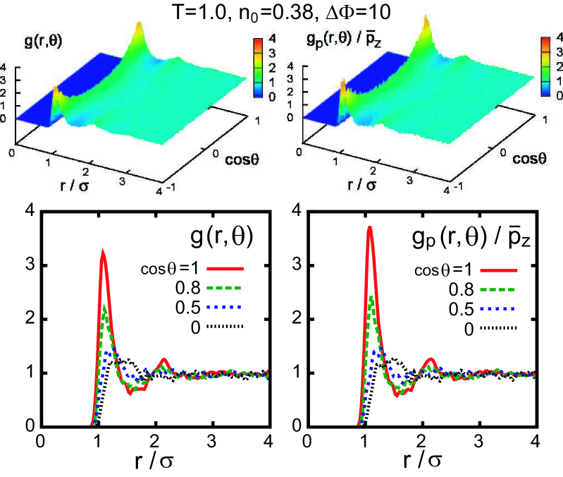
From the first term in Eq.(3.11), the short-range part of the local field in the interior is given by ${\mbox{\boldmath$E$}}_{i}^{\rm ds}\cong-\sum_{j\neq i}\stackrel{{\scriptstyle\leftrightarrow}}{{w}}_{s}(|{\mbox{\boldmath$r$}}_{ij}|)\cdot{\mbox{\boldmath$\mu$}}_{j}$, where the contributions with ${\mbox{\boldmath$m$}}\neq(0,0,0)$ are neglected. From Eqs.(3.4) and (3.33) the lateral average of its $z$ component is written in terms of $g_{\rm p}(r,\theta)$ for $\Delta z\ll 1$ as

$$\langle{E_{z}^{\rm ds}}\rangle\cong\int d{\mbox{\boldmath$r$}}[C(r)\cos^{2}\theta-B(r)]g_{\rm p}(r,\theta).$$ (3.35)

If we set $g_{\rm p}(r,\theta)={\bar{p}}_{z}$, the integral is nearly equal to $4\pi{\bar{p}}_{z}/3$ from Eq.(3.5) Lorentz . Use of Eq.(3.25) yields the correction to the classical value in the form,

$$\gamma_{\rm\ell}-\frac{1}{3}\cong\int\frac{d{\mbox{\boldmath$r$}}}{4\pi}[C(r)\cos^{2}\theta-B(r)][\frac{g_{\rm p}(r,\theta)}{{\bar{p}}_{z}}-1].$$ (3.36)

Here, we may well replace $C(r)\cos^{2}\theta-B(r)$ by $(3\cos^{2}\theta-1)/r^{3}$, since ${g_{\rm p}(r,\theta)}/{{\bar{p}}_{z}}-1$ is small for $r/\sigma\gtrsim\gamma^{-1}$ in Fig.10. In Table 1, the above formula reproduces the numerical values of $\gamma_{\ell}$ with errors of order $10\%$.

III.3.3 Dipole chains

Figure 11: (Color online) Chains of 1000 spherical dipoles at $T=0.2$ for $n_{0}=0.19$ in a $L\times L\times H$ cell ($H=L$). Potential difference $\Delta\Phi$ is set equal to 0, 8, 10, and 100. For small $\Delta\Phi$ dipoles parallel and antiparallel to the $z$ axis are both attracted and aligned by the image interaction near the walls. They are written in white or in gray, respectively. For large $\Delta\Phi$, they are aligned along the $z$ axis.

Figure 12: (Color online) Chains of 1000 spherical dipoles at $T=0.2$ for $n_{0}=0.57$ in a $L\times L\times H$ cell ($H=L$) for $\Delta\Phi=0$ (left) and 10 (right). Shown also are cross-sectional configurations in the bottom two layers, $0<z<1$ and $1<z<2$, in (b) and (b^′) and those in the middle two layers, $H/2+1<z<H/2+2$ and $H/2<z<H/2+1$, in (c) and (c^′). White (gray) particles are parallel (antiparallel) to the $z$ axis. Colors are lighter for dipoles in the second layers.

Figure 13: (Color online) Mean square displacements for the particles near the walls and those far from them for $\Delta\Phi=0$ (left) and 10 (right), where $T=0.2$ and $n_{0}=0.57$. The data are the same as in Fig.12. Time $t$ is in units of $\tau_{0}$ in Eq.(2.40).

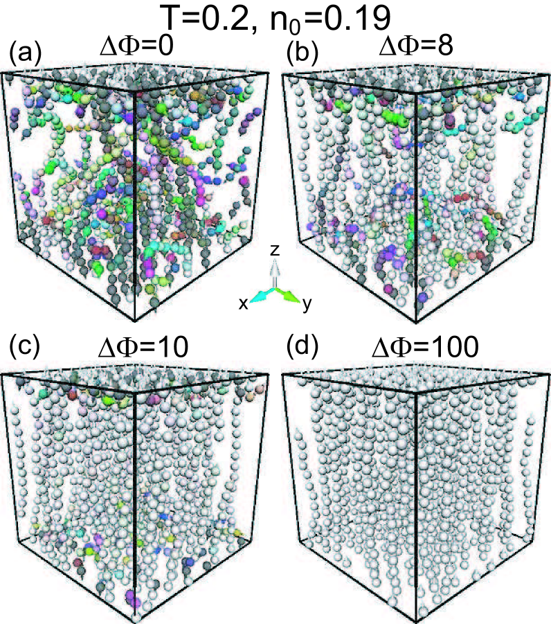
For ferromagnetic particles with permanent dipoles, chain formation was predicted PG and has been studied numerically Weis ; Mazars ; KlappJCP . As electrorheological fluids, use has been made of colloids with a dielectric constant different from that of the surrounding fluid Hasley ; Martin , which have induced dipole moments in electric field. Coating of colloids with urea (with a high molecular dipole moment of 4.6D) is known to increase the polarizability Shen . Experiments on such dielectric particles have been performed extensively, but simulations including the image interaction under applied electric field were performed only for induced point dipoles oriented along the $z$ axisTao . Here, we present simulation results on permanent point dipoles. We show that they are attracted to the walls by the image dipoles and the surface charges due to the applied electric field.

In Fig.11, we gives our examples of dipole chains at $T=0.2$ for $n_{0}=0.19$ under four potential differences $\Delta\Phi=0$, 8, 10, and 100. For $\Delta\Phi=0$ in (a), chains are formed near the walls, where dipoles are attracted to the walls and aligned in the directions parallel or antiparallel to the $z$ axis due to the image interaction (3.7). For $\Delta\Phi=8$ in (b), even dipoles away from the walls form strings along the $z$ axis. For $\Delta\Phi=10$ in (c), chains are stretched between the two plates, but antiparallel wall attachments still occur. For $\Delta\Phi=100$ in (d), all the dipoles are aligned along the $z$ axis.

We consider the average dipole moment over all the particles and that over those at the bottom defined by

$$\langle{\mu_{z}}\rangle_{\rm all}=\sum_{i}\mu_{zi}/N,\quad\langle{\mu_{z}}\rangle_{\rm wall}=\sum_{0<z_{i}<1}\mu_{zi}/N_{\rm w},$$ (3.37)

where $N_{\rm w}$ is the particle number in the layer $0<z_{i}<1$. For the data in Fig.11, we obtain $(\langle{\mu_{z}}\rangle_{\rm all},\langle{\mu_{z}}\rangle_{\rm wall})=(0,0),(0.67,0.09),(1.34,0.27),(1.91,0.69),(1.97,1.97)$ for $\Delta\Phi=0$, 8, 10, 100, respectively. Here, we estimate the image interaction energy as $|v_{\rm I}^{\rm d}|\sim 4$ for $z_{i}\sim 0.5$ from Eq.(3.7) and the typical field energy as $\mu_{0}E_{a}\sim 0.2\Delta\Phi$. Comparison of these two energies yields a crossover potential difference about 20, in accord with Fig.11.

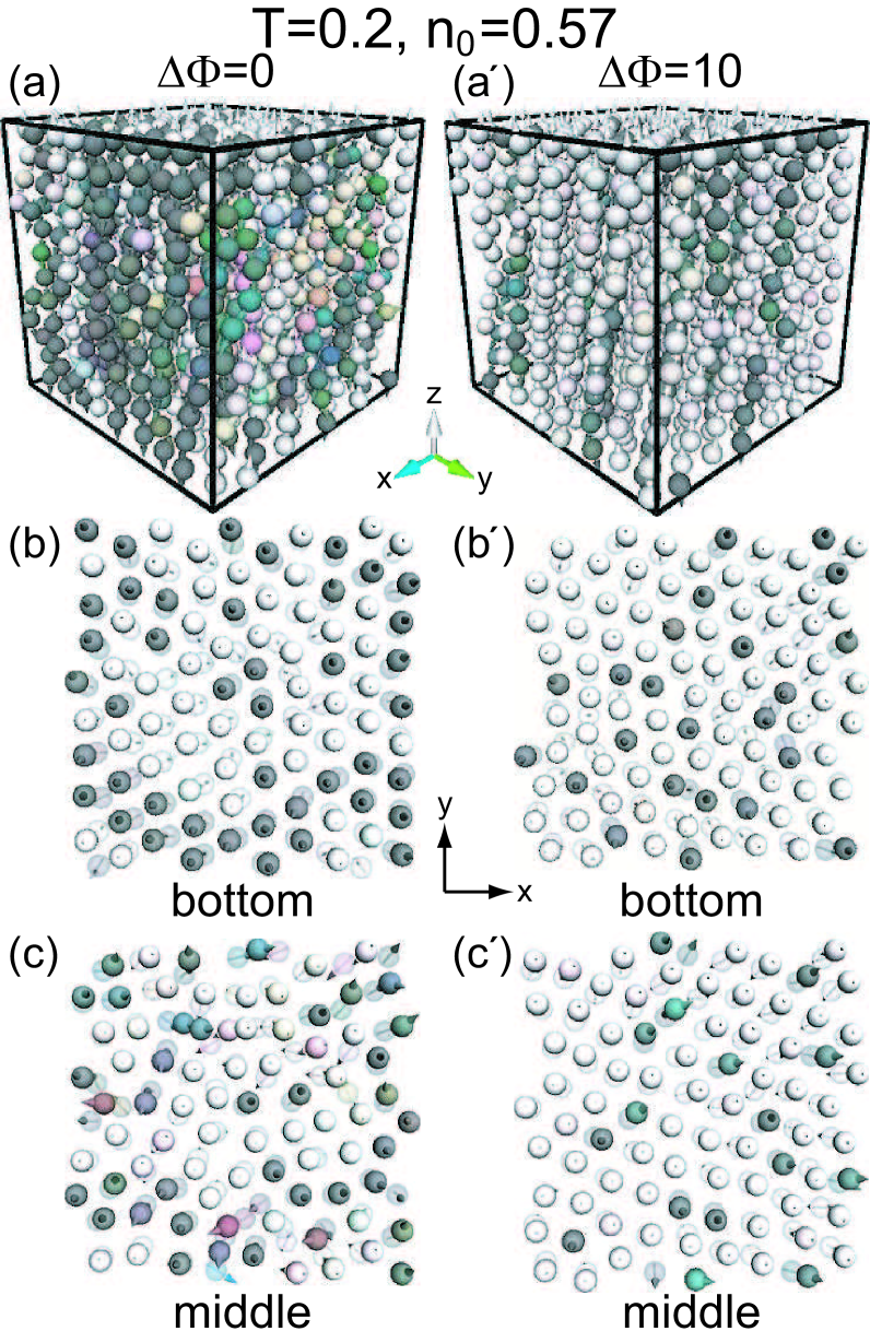
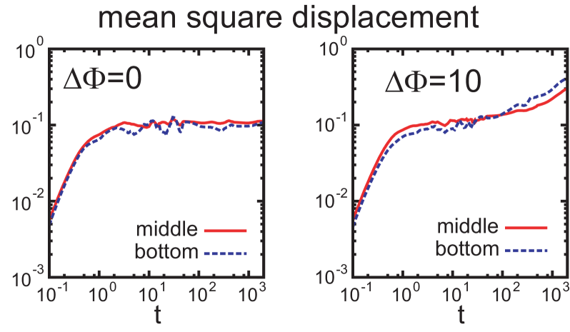
In Fig.12, we show dipole configurations for $n_{0}=0.57$ under two potential differences $\Delta\Phi=0$ and 10. At this high density, a hexagonal lattice (with defects) appears on the walls, extending between the top and the bottom in the form of chains. For $\Delta\Phi=0$, the cross-sectional configurations in the middle are glassy. We can see that the chains are somewhere curved, broken, branched, or even entangled. In the left panel of Fig.13, we plot the mean-square displacement,

$$M(t)=\langle{|{\mbox{\boldmath$r$}}_{i}(t+t_{0})-{\mbox{\boldmath$r$}}_{i}(t_{0})|^{2}}\rangle,$$ (3.38)

where the average over $t_{0}(<10^{4})$ was taken. Furthermore, we took the average over the particles close to the walls and that over those in the interior separately, but there was no essential difference for these two groups of the particles, as shown in Fig.13. We notice that $M(t)$ grows to saturate at a plateau value ($\sim 0.1$) for $t\gtrsim 1$ in units of $\tau_{0}$ in Eq.(2.40). We can also see a tendency of segregation between the chains parallel to the $z$ axis and those antiparallel to the $z$ axis. On the other hand, for $\Delta\Phi=10$, the fraction of the chains parallel to the $z$ axis increases and the orientational fluctuations decrease, where $\langle{\mu_{z}}\rangle_{\rm all}=1.17$ and $\langle{\mu_{z}}\rangle_{\rm wall}=0.99$ (see Eq.(3.37)). In this more ordered state, collective configuration changes are appreciable for $t\gtrsim 100$. In the right panel of Fig.13, this leads to very slow growth of $M(t)$.

IV Summary and remarks

In summary, we have extended the Ewald method for charged and polar particles between metallic plates in a $L\times L\times H$ cell, aiming to apply electric field $E_{a}$ to these systems. In this problem, we should account for an infinite number of image charges and dipoles outside the cell. With this method, we have presented some results of molecular dynamics simulation.

In the previous papers by Hautman et al.Hautman , by Perram and RatnerPerram , and by Klapp Klapp , the conventional 3D Ewald method for periodic systems was applied to a doubly expanded $L\times L\times 2H$ cell, where the three axes were formally equivalent. Our scheme is essentially the same as theirs, but we have treated the $z$ direction differently from the lateral directions. In particular, we have divided the terms in the long-range part of the Ewald sum into those inhomogeneous in the $xy$ plane (with nonvanishing $k_{x}$ or $k_{y}$) and those homogeneous in the $xy$ plane but inhomogeneous along the $z$ axis (with $k_{x}=k_{y}=0$ and $k_{z}\neq 0$) in Eqs.(2.26) and (3.11). The latter one-dimensional terms can be summed into simple forms in Eqs.(2.28) and (3.12), yielding the one-dimensional electric field $E_{i}^{0}$ in Eqs.(2.33) and (3.15). In our simulations, we have calculated $E_{i}^{0}$ very accurately. For dipole systems, $E_{i}^{0}\cong E_{a}$ far from the walls for thick cells.

In applying electric field between metallic plates, we may control the potential difference $\Delta\Phi=HE_{a}$ or the surface charge $Q_{0}$. The electrostatic energy, $U_{\rm m}$ or $U_{\rm m}^{\rm d}$, in the fixed-potential condition is related to that in the fixed-charge condition by the Legendre transformation, as shown in Appendix B. In the continuum electrostatics in Appendix D, we have also introduced the free energies $F_{\rm m}$ and $F_{\rm e}$ for these two cases Landau ; OnukiNATO .

Some remarks are given below.
(1) We have assumed stationary applied field, but we may assume a time-dependent field $E_{a}(t)$ and examine various nonequilibrium phenomena. For example, when $\Delta\Phi$ was changed from 0 to 100, we observed complex dynamics of charged particles from the crystal in Fig.4(a) to that in Fig.4(a^′). We also mention that melting due to electric field was observed in charged colloidal crystal super .
(2) We have assumed spherical dipoles, but real molecules are nonspherical and undergo hindered rotations. This feature should be included in future simulations. We should also consider mixtures of ions and nonspherical polar molecules bounded by metallic plates, where the ion-dipole interaction is crucial Is ; Onuki .
(3) The classical result $\gamma_{\ell}=1/3$ for the local field factor follows for a spherical cavity Onsager ; Kirk , leading to the Clausius-Mossotti formula for the dielectric constant. However, $\gamma_{\ell}$ becomes one of the depolarization factors for an ellipsoidal cavitylocal , so it is sensitive to the environment around each dipole. In our case, $\gamma_{\ell}$ increases due to the pair correlations along the applied field as in Eq.(3.36). More systematic simulations are needed on this aspect.
(4) Various systems such as charged colloids, polyelectrolytes, proteins, and water molecules should exhibit interesting behaviors close to metal surfaces without and with applied field colloid ; Corni ; Messina . For polarizable surfaces, a simulation method similar to ours has recently been reported double .
(5) We may well expect ferroelectric phase transitions in confined dipole systems (see the sentences below Eq.(3.29)). Furthermore, it is of great interest to examine the electric field effects in ferroelectric systems with impurities. We will shortly report on the electric field effect in orientational glass as a continuation of our previous work EPL .

Appendix A: Derivation of Eq.(2.7)

The last two terms in Eq.(2.7) arise from the long-range part of the electrostatic energy, written as $U_{\rm p}^{\ell}$. We transform it as follows:

$$U_{\rm p}^{\ell} = \frac{1}{2}\sum_{\mbox{\boldmath$m$}}{\sum_{i,j}}{q_{i}q_{j}}\psi_{\ell}({|{\mbox{\boldmath$r$}}_{ij}+L{\mbox{\boldmath$m$}}|})$$ (A1)

$$= \frac{1}{2}\int_{\mbox{\boldmath$k$}}\Psi_{\ell}(k)\sum_{\mbox{\boldmath$m$}}{\sum_{i,j}}{q_{i}q_{j}}e^{{\rm i}{\mbox{\boldmath$k$}}\cdot({{\mbox{\boldmath$r$}}_{ij}+L{\mbox{\boldmath$m$}}})},$$

where $\int_{\mbox{\boldmath$k$}}=(2\pi)^{-3}\int d{\mbox{\boldmath$k$}}$ and $\Psi_{\ell}(k)$ is defined in Eq.(2.8). In the second line, we perform the summation over $m$ introducing a damping factor $\exp[{-\epsilon|m_{x}|-\epsilon|m_{y}|-\epsilon|m_{z}|}]$, where $\epsilon$ is a positive small number (not to be confused with the energy $\epsilon$ in $v_{s}(r)$ in Eq.(2.36)). The summation yields $\sum_{\mbox{\boldmath$m$}}\exp({{\rm i}{\mbox{\boldmath$k$}}\cdot L{\mbox{\boldmath$m$}}})=\zeta(Lk_{x})\zeta(Lk_{y})\zeta(Lk_{z})$, where

$$\zeta(u) = \sum_{m_{x}=0,\pm 1,\cdots}\exp[{\rm i}m_{x}u-\epsilon|m_{x}|)$$ (A2)

$$\cong{2\epsilon}/[{\epsilon^{2}+2(1-\cos(u))}].$$

For $Lk>1$, $\Psi_{\ell}(k)$ is finite, so we may replace $\zeta(Lk_{\alpha})$ by $2\pi\sum_{\nu_{\alpha}\neq 0}\delta(Lk_{\alpha}-2\pi\nu_{\alpha})$, where $\alpha=x,y,z$. For $Lk\lesssim 1$, we may set $\zeta(Lk_{\alpha})={2\epsilon}/[{\epsilon^{2}+L^{2}k_{\alpha}^{2}}]$. Thus, $U_{\rm p}^{\ell}$ becomes

$$U_{\rm p}^{\ell} = \frac{1}{2}\int_{\mbox{\boldmath$k$}}\Psi_{\ell}(k)\zeta(Lk_{x})\zeta(Lk_{y})\zeta(Lk_{z}){\sum_{i,j}}{q_{i}q_{j}}e^{{\rm i}{\mbox{\boldmath$k$}}\cdot{\mbox{\boldmath$r$}}_{ij}}$$ (A3)

$$= \frac{1}{2L^{3}}\sum_{{\mbox{\boldmath$k$}}\neq{\mbox{\boldmath$0$}}}\Psi_{\ell}(k){\sum_{i,j}}{q_{i}q_{j}}e^{{\rm i}{\mbox{\boldmath$k$}}\cdot{\mbox{\boldmath$r$}}_{ij}}$$

$$+\int_{\mbox{\boldmath$k$}}\frac{16\pi\epsilon^{3}{\sum_{i,j}}{q_{i}q_{j}}[e^{{\rm i}{\mbox{\boldmath$k$}}\cdot{{\mbox{\boldmath$r$}}_{i}}}-1][e^{-{\rm i}{\mbox{\boldmath$k$}}\cdot{{\mbox{\boldmath$r$}}_{j}}}-1]}{k^{2}({\epsilon^{2}+L^{2}k_{x}^{2}})({\epsilon^{2}+L^{2}k_{y}^{2}})({\epsilon^{2}+L^{2}k_{z}^{2}})}.$$

The first term coincides with the third term in Eq.(2.7) with ${\mbox{\boldmath$k$}}=2\pi L^{-1}(\nu_{x},\nu_{y},\nu_{z})\neq{(0,0,0)}$. The second term arises from $k\lesssim L^{-1}$, where $\exp[{{\rm i}{\mbox{\boldmath$k$}}\cdot{\mbox{\boldmath$r$}}_{i}}]-1\cong{{\rm i}{\mbox{\boldmath$k$}}\cdot{\mbox{\boldmath$r$}}_{i}}$ and $\exp[-{{\rm i}{\mbox{\boldmath$k$}}\cdot{\mbox{\boldmath$r$}}_{j}}]-1\cong-{{\rm i}{\mbox{\boldmath$k$}}\cdot{\mbox{\boldmath$r$}}_{j}}$ for small $k$. Furthermore, ${k}_{\alpha}{k}_{\beta}$ may be replaced by $(k^{2}/3)\delta_{\alpha\beta}$ from the angle integration of $k$, leading to the fourth term in Eq.(2.7).

Appendix B: Fixed charge boundary condition

As illustrated in Fig.1, we may fix the surface changes, $Q_{0}$ and $Q_{H}$, at $z=0$ and $H$ Landau ; OnukiNATO , as well as the potential difference $\Delta\Phi$. Here, we consider the fixed charge boundary condition, where we assume $Q_{H}=-Q_{0}$ without ionization on the surfaces. See Appendix D for the continuum theory for these two boundary conditions.

For charged particles, let $U_{\rm e}=U_{\rm e}({\mbox{\boldmath$r$}}_{1},\cdots,Q_{0})$ be the electrostatic energy appropriate for the fixed-charge condition, which includes the contribution from the excess electrons on the metal surfaces. For infinitesimal changes ${\mbox{\boldmath$r$}}_{i}\to{\mbox{\boldmath$r$}}_{i}+d{\mbox{\boldmath$r$}}_{i}$ and $Q_{0}\to Q_{0}+dQ_{0}$, $U_{\rm e}$ is changed as

$$dU_{\rm e}=-\sum_{i}q_{i}{\mbox{\boldmath$E$}}_{i}\cdot d{\mbox{\boldmath$r$}}_{i}+HE_{a}dQ_{0},$$ (B1)

where $E_{a}$ is a dynamic variable at fixed $Q_{0}$. The expressions for ${\mbox{\boldmath$E$}}_{i}$ are the same in the two cases at fixed $E_{a}$ and at fixed $Q_{0}$. Then, from Eqs.(2.24) and (B1), $U_{\rm e}$ and $U_{\rm m}$ are related by

$$U_{\rm e}=U_{\rm m}-HL^{2}E_{a}^{2}/8\pi+HE_{a}Q_{0}.$$ (B2)

For dipoles, the electrostatic energy $U_{\rm e}^{\rm d}$ under the fixed-charge condition satisfies

$$dU_{\rm e}^{\rm d}=-\sum_{i}({\mbox{\boldmath$F$}}_{i}^{e}\cdot d{\mbox{\boldmath$r$}}_{i}+{\mbox{\boldmath$E$}}_{i}\cdot d{\mbox{\boldmath$\mu$}}_{i})+HE_{a}dQ_{0},$$ (B3)

which should be compared with Eq.(3.10). As in Eq.(B2), $U_{\rm e}^{\rm d}$ and $U_{\rm m}^{\rm d}$ are related by

$$U_{\rm e}^{\rm d}=U_{\rm m}^{\rm d}-HL^{2}E_{a}^{2}/8\pi+HE_{a}Q_{0}.$$ (B4)

Appendix C: Derivation of Eq.(2.28)

In Eq.(2.26), $K_{0}(z,z^{\prime})$ is given by the lateral integral,

$$K_{0}(z,z^{\prime})=\frac{1}{4\pi}\int dxdy\sum_{\mbox{\boldmath$m$}}[\psi_{\ell}({|{\mbox{\boldmath$r$}}-{\mbox{\boldmath$r$}}^{\prime}+{\mbox{\boldmath$h$}}|})$$

$$\hskip 56.9055pt-\psi_{\ell}({|{{\mbox{\boldmath$r$}}}-{\bar{\mbox{\boldmath$r$}}}^{\prime}+{\mbox{\boldmath$h$}}|})],$$ (C1)

where ${\mbox{\boldmath$r$}}=(x,y,z)$, ${{\mbox{\boldmath$r$}}}^{\prime}=(x^{\prime},y^{\prime},z^{\prime})$, ${\bar{\mbox{\boldmath$r$}}}^{\prime}=(x^{\prime},y^{\prime},-z^{\prime})$, and $0<x,y<L$.After the integration, the right hand side becomes a function of $z$ and $z^{\prime}$ independent of $x^{\prime}$ and $y^{\prime}$. We then twice differentiate $K_{0}(z,z^{\prime})$ with respect to $z$ and use the relation $\nabla^{2}\psi_{\ell}(r)=-4\pi\varphi(x)\varphi(y)\varphi(z)$, where $\varphi(x)$ is defined by Eq.(2.5). Some calculations yield

$$\frac{\partial^{2}}{\partial z^{2}}K_{0}(z,z^{\prime})=-\hat{\varphi}(z-z^{\prime})+\hat{\varphi}(z+z^{\prime}),$$ (C2)

where $\hat{\varphi}(z)$ is defined by Eq.(2.29). The above relation is integrated to give Eq.(2.28) under $K_{0}(0,z^{\prime})=K_{0}(H,z^{\prime})=0$. Furthermore, Eqs.(2.19) and (2.28) give

$$\frac{\partial K_{0}(z,z^{\prime})}{\partial z^{\prime}}=\int_{0}^{z}du[\hat{\varphi}(u+z^{\prime})+\hat{\varphi}(u-z^{\prime})]-\frac{z}{H},$$ (C3)

$$\frac{\partial^{2}K_{0}(z,z^{\prime})}{\partial z\partial z^{\prime}}=\hat{\varphi}(z+z^{\prime})+\hat{\varphi}(z-z^{\prime})-\frac{1}{H},$$ (C4)

where we have used $\int_{0}^{H}du[\hat{\varphi}(u+z^{\prime})+\hat{\varphi}(u-z^{\prime})]=1$ from the periodicity of $\hat{\varphi}(u)$.

Appendix D: Continuum theory of electrostatics

We compare the results in the text and those of continuum electrostatics Landau ; OnukiNATO . We consider charged particles in a polar medium between parallel metallic plates under applied electric field $E_{a}$. The system is in the region $0<x,y<L$ and $0<z<H$. We assume $L\gg H$ to neglect the edge effect. We do not assume the (artificial) periodic boundary condition in the $x$ and $y$ axes.

In this appendix, the physical quantities are smooth functions of space after spatial coarse-graining. In addition to the electrostatic potential $\Phi({\mbox{\boldmath$r$}})=\phi({\mbox{\boldmath$r$}})-E_{a}z$, we introduce the charge density $\rho({\mbox{\boldmath$r$}})$ and the polarization ${\mbox{\boldmath$p$}}({\mbox{\boldmath$r$}})$. The electric field ${\mbox{\boldmath$E$}}=-\nabla\Phi=E_{a}{\mbox{\boldmath$e$}}_{z}-\nabla\phi$ and the electric induction ${\mbox{\boldmath$D$}}={\mbox{\boldmath$E$}}+4\pi{\mbox{\boldmath$p$}}$ are defined. For simplicity, we assume the overall charge neutrality condition $\int d{\mbox{\boldmath$r$}}\rho=0$ without ionization on the walls. Hereafter, the integral $\int d{\mbox{\boldmath$r$}}$ is performed within the cell.

From the relation $\nabla\cdot{\mbox{\boldmath$D$}}=4\pi\rho$, we may define the effective charge density by

$$\rho_{e}=\rho-\nabla\cdot{\mbox{\boldmath$p$}},$$ (D1)

which satisfies $\nabla\cdot{\mbox{\boldmath$E$}}=-\nabla^{2}\phi=4\pi\rho_{e}$. Let $\rho_{e{\mbox{\boldmath$k$}}}(z)=\int d{\mbox{\boldmath$r$}}_{\perp}e^{-{\rm i}{\mbox{\boldmath$k$}}\cdot{\mbox{\boldmath$r$}}_{\perp}}\rho_{e}$ be the 2D Fourier transformation in the $xy$ plane, where ${\mbox{\boldmath$k$}}=(k_{x},k_{y})$ and ${\mbox{\boldmath$r$}}_{\perp}=(x,y)$. As in Eq.(2.16), the excess potential $\phi$ is written as

$$\phi({\mbox{\boldmath$r$}})=4\pi\int_{\mbox{\boldmath$k$}}\int_{0}^{H}dz^{\prime}G_{k}(z,z^{\prime})\rho_{e{\mbox{\boldmath$k$}}}(z^{\prime})e^{{\rm i}{\mbox{\boldmath$k$}}\cdot{\mbox{\boldmath$r$}}_{\perp}},$$ (D2)

where $\int_{\mbox{\boldmath$k$}}=(2\pi)^{-2}\int dk_{x}dk_{y}$ and the Green function $G_{k}(z,z^{\prime})$ is given in Eq.(2.18).

First, we consider the lateral averages ($0<x,y<L$),

$$\bar{\phi}(z)=\int dxdy~{}\phi/L^{2},\quad\bar{p}_{z}(z)=\int dxdy~{}p_{z}/L^{2},$$

$$\bar{\rho}(z)=\int dxdy~{}\rho/L^{2},\quad{\bar{\rho}}_{e}(z)=\int dxdy~{}\rho_{e}/L^{2}.$$ (D3)

Then, we find $\bar{\rho}_{e}={\bar{\rho}}-d{\bar{p}}_{z}/dz$ and Eq.(D2) becomes

$${\bar{\phi}}(z)=4\pi\int_{0}^{H}duG_{0}(x,u){\bar{\rho}}_{e}(u),$$ (D4)

where $G_{0}(z,z^{\prime})$ is given in Eq.(2.19). The average electric field $\bar{E}_{z}(z)=E_{a}-d\bar{\phi}(z)/dz$ is calculated as

$${{\bar{E}}_{z}(z)}=-{4\pi}{\bar{p}}_{z}(z)+4\pi Q_{0}/L^{2}+4\pi\int_{0}^{z}du{\bar{\rho}}(u).$$ (D5)

The total surface charge at $z=0$ is denoted by $Q_{0}$; then, that at $z=H$ is $Q_{H}=-Q_{0}$. From Eq.(D4) we obtain commentS

$$Q_{0}=\frac{L^{2}}{4\pi}E_{a}+\frac{1}{H}\int d{\mbox{\boldmath$r$}}[z{\rho}({\mbox{\boldmath$r$}})+{p}_{z}({\mbox{\boldmath$r$}})].$$ (D6)

This formula corresponds to Eqs.(2.31) and (3.17). The above relation itself readily follows if we set $\rho=\nabla\cdot{\mbox{\boldmath$D$}}/4\pi$ in the integral $\int d{\mbox{\boldmath$r$}}z\rho$.

Second, we consider the electrostatic energy $U_{\rm m}$ in the fixed-potential condition. Its discrete versions are in Eqs.(2.23) and (3.9). The continuum version reads

$$U_{\rm m}=\int d{\mbox{\boldmath$r$}}[\frac{1}{2}\rho_{e}\phi-E_{a}(z\rho+p_{z})].$$ (D7)

For small incremental changes ($\rho\to\rho+\delta\rho,{\mbox{\boldmath$p$}}\to{\mbox{\boldmath$p$}}+\delta{\mbox{\boldmath$p$}},....)$, $U_{\rm m}$ in Eq.(D7) is changed as

$$\delta U_{\rm m}=\int d{\mbox{\boldmath$r$}}[\Phi\delta\rho-{\mbox{\boldmath$E$}}\cdot\delta{\mbox{\boldmath$p$}}-(z\rho+p_{z})\delta E_{a}],$$ (D8)

which corresponds to Eqs.(2.24) and (3.10). On the other hand, the electrostatic energy $U_{\rm e}$ in the fixed-charge condition should satisfy

$$\delta U_{\rm e}=\int d{\mbox{\boldmath$r$}}(\Phi\delta\rho-{\mbox{\boldmath$E$}}\cdot\delta{\mbox{\boldmath$p$}})+HE_{a}\delta Q_{0},$$ (D9)

which is the counterpart of Eqs.(B1) and (B3). Then, $U_{\rm e}$ and $U_{\rm m}$ are related by Eq.(B2) or (B4), leading toOnukiNATO ; Landau

$$U_{\rm e}=U_{\rm m}-\frac{HL^{2}}{8\pi}E_{a}^{2}+HE_{a}Q_{0}=\int d{\mbox{\boldmath$r$}}\frac{|{\mbox{\boldmath$E$}}|^{2}}{8\pi}.$$ (D10)

Third, we remark on the polarization $p$. So far it has been treated as an independent variable. Without ferroelectric order, $p$ is usually related to $E$ by Landau ,

$${\mbox{\boldmath$p$}}=\chi{\mbox{\boldmath$E$}},$$ (D11)

in the linear response regime. From ${\mbox{\boldmath$D$}}=\varepsilon{\mbox{\boldmath$E$}}$, the electric susceptibility $\chi$ and the dielectric constant $\varepsilon$ are related by $\varepsilon=1+4\pi\chi.$ In this situation, we may introduce the following free energy contribution,

$$F_{\rm p}=\int d{\mbox{\boldmath$r$}}\frac{1}{2\chi}|{\mbox{\boldmath$p$}}|^{2},$$ (D12)

which is an increase in the free energy due to mesoscopic ordering of the constituting dipoles. The polarization free energy is needed to examine the thermal fluctuations of $p$Fel ; OnukiNATO . We then treat the sum, $F_{\rm m}=U_{\rm m}+F_{\rm p}$ or $F_{e}=U_{\rm e}+F_{\rm p}$, as the electrostatic free energy in the fixed-potential or fixed-charge condition. Since its functional derivative with respect to $p$ is given by $-{\mbox{\boldmath$E$}}+\chi^{-1}{\mbox{\boldmath$p$}}$ from Eqs.(D8), (D9), and (D12), its minimization yields Eq.(D11). Eliminating $p$, we rewrite $F_{\rm m}$ and $F_{\rm e}$ as

$$F_{\rm m}=\int d{\mbox{\boldmath$r$}}(\rho\Phi-\frac{\varepsilon}{8\pi}|\mbox{\boldmath$E$}|^{2})+\frac{HL^{2}}{8\pi}E_{a}^{2},$$ (D13)

$$F_{{\rm e}}=\int d{\mbox{\boldmath$r$}}\frac{\varepsilon}{8\pi}|{\mbox{\boldmath$E$}}|^{2}.$$ (D14)

The second term in $F_{\rm m}$ in Eq.(D13) is a constant at fixed $E_{a}$, so we may redefine the electrostatic free energy as

$$F_{\rm m}^{\prime}=F_{\rm m}-HL^{2}E_{a}^{2}/8\pi=F_{\rm e}-Q_{0}(\partial F_{\rm e}/\partial Q_{0}),$$ (D15)

which is the Legendre transform of $F_{\rm e}$. The two expressions, $F_{\rm m}^{\prime}$ and $F_{\rm e}$, have both been used in the literature. In the Ginzburg-Landau scheme, Yaakov et al.Yaakov used $F_{\rm m}^{\prime}$ and one of the present authorsOnuki used $F_{\rm e}$ for ions in a mixture solvent, where $\varepsilon$ depends on the local solvent composition and is inhomogeneous.

References

- (1) J. N. Israelachvili, Intermolecular and Surface Forces (Academic Press, London, 1991).
- (2) M. P. Allen and D. J. Tildesley, Computer Simulation of Liquids (Clarendon Press, Oxford, 1987).
- (3) D. Frenkel and B. Smit, Understanding Molecular Simulation, Second Edition: From Algorithms to Applications (Academic Press, San Diego,1996).
- (4) P. P. Ewald, Annalen der physik, 369, 253 (1921).
- (5) S. W. de Leeuw, J. W. Perram, and E. R. Smith, Proc. R. Soc. Lond. A. 373, 27 (1980).
- (6) S. W. de Leeuw, J. W. Perram, and E. R. Smith, Annu. Rev. Phys. Chem. 37, 245 (1986).
- (7) J.-J. Weis and D. Levesque, Adv. Polym. Sci. 185, 163 (2005).
- (8) M. Mazars, Physics Reports 500, 43 (2011).
- (9) D. Parry, Surf. Sci. 49, 433 (1975); D. M. Heyes, M. Barber, and J. H. R. Clarke, J. Chem. Soc., Faraday Trans. 2 73, 1485 (1977); S. W. de Leeuw and J. W. Perram, Physica A 113, 546 (1982).
- (10) E. R. Smith, Mol. Phys. 65, 1089 (1988); A. H. Widmann and D. B. Adolf, Comput. Phys. Commun. 107, 167 (1997); Y. J. Rhee, J. W. Halley, J. Hautman, and A. Rahman, Phys. Rev. B, 40, 36 (1989).
- (11) I.-C. Yeh and M. L. Berkowitz, J. Chem. Phys. 111, 3155 (1999); A. Arnold, J. de Joannis, and C. Holm, J. Chem. Phys. 117, 2496 (2002).
- (12) P. S. Crozier, R. L. Rowley, E. Spohr, D. Henderson, J. Chem. Phys. 112, 9253 (2000).
- (13) S. H. L. Klapp and M. Schoen, J. Chem. Phys. 117, 8050 (2002).
- (14) S. Tyagi, A. Arnold, and C. Holm, J. Chem. Phys. 127, 154723 (2007).
- (15) E. R. Smith, J. Chem. Phys. 128, 174104 (2008).
- (16) L. D. Landau and E. M. Lifshitz, Electrodynamics of Continuous Media (Pergamon, 1984).
- (17) J. Hautman, J. W. Halley, Y.-J. Rhee, J. Chem. Phys., 91, 467 (1989). These authors also found that the contribution from vanishes in the long-range Ewald sum of the electrostatic energy (see the appendix in their paper).
- (18) J. W. Perram and M. A. Ratner, J. Chem. Phys.104, 5174 (1996). These authors obtained . This expression is equivalent to ours in Eq.(2.17).
- (19) S. H. L. Klapp, Mol. Simul. 32, 609 (2006).
- (20) T. C. Halsey and W. Toor, Phys. Rev. Lett. 65, 2820 (1990); T. C. Hasley, Science 258, 761 (1992).
- (21) R. Tao and J. M. Sun, Phys. Rev. Lett. 67, 398 (1991). G. L. Gulley and R. Tao, Phys. Rev E 56, 4328 (1997).
- (22) F. Iori and S. Corni, J. Comput. Chem. 29, 1656 (2008).
- (23) R. Messina, J. Phys.: Condens. Matter 21, 113102 (2009).
- (24) R. Messina, J. Chem. Phys. 117, 11062 (2002); A. P. dos Santos, A. Bakhshandeh, and Y. Levin, J. Chem. Phys. 135, 044124 (2011); L. Lue and P. Linse, J. Chem. Phys. 135, 224508 (2011); Z. Gan, X. Xing, and Z. Xu, J. Chem. Phys. 137, 034708 (2012).
- (25) A. Onuki, in Nonlinear Dielectric Phenomena in Complex Liquids, edited by S. J. Rzoska and V. Zhelezny (Kluwer Academic Publishers, Dordrecht, 2004).
- (26) L. Onsager, J. Am. Chem. Soc. 58, 1486 (1936).
- (27) J. G. Kirkwood, J. Chem. Phys. 7, 911 (1939).
- (28) D. Wei, Phys. Rev.E 49 ,2454 (1994); M. J. Stevens and G. S. Grest, Phys. Rev.E 51, 5976 (1995); V. V. Murashov and G. N. Patey, J. Chem. Phys. 112, 9828 (2000); Z. Wang, C. Holm, and H. W. Mller, Phys. Rev. E 66, 021405 (2002); J. Jordanovic and S. H. L. Klapp, Phys. Rev.E 79, 021405 (2009). J. Richardi and J.-J. Weis, J. Chem. Phys. 135, 124502 (2011).
- (29) M. E. Leunissen, C. G. Christova, A.-P. Hynninen, C. P. Royall, A. I. Campbell, A. Imhof, M. Dijkstra, R. van Roij, and A. van Blaaderen, Nature 437, 235 (2005).
- (30) P. G. de Gennes and P. A. Pincus, Phys. Kondens. Mater. 11, 189 (1970).
- (31) M. Deserno and C. Holm, J. Chem. Phys. 109, 7678 (1998).
- (32) In the Debye-Hckel theory of electrolytes, the potential decays as or far from the walls for , where is the Debye wave number. In this theory the ratio of to is .
- (33) K. Takae and A. Onuki, EPL 100, 16006 (2012).
- (34) For the examples in Table 1, the ratio is given by , ,, , , and from above.
- (35) C. V. Raman and K. S. Krishnan, Philos. Mag. 5, 498 (1928); A. K. Burnham, G. R. Alms, and W. H. Flygare, J. Chem. Phys. 62, 3289 (1975).
- (36) J. P. Huang, Z. W. Wang, and C. Holm, Phys. Rev. E 71, 061203 (2005); E. A. Elfimova, A. O. Ivanov, and P. J. Camp, J. Chem. Phys. 136, 194502 (2012).
- (37) In our simulation, the cut-off length for the short-range part of the electrostatic interaction is . For , the integral of in the range is nearly equal to 1.
- (38) J. E. Martin, J. Odinek, and T. C. Halsey, Phys. Rev. Lett. 69, 1524 (1992).
- (39) W. Wen, X. Huang, S. Yang, K. Lu, and P. Sheng, Nat. Mater. 2, 727 (2003).
- (40) A. Onuki, Phys. Rev. 73, 021506 (2006); J. Chem. Phys. 128, 224704 (2008). In these papers, the image interaction is taken into account at a liquid-liquid interface.
- (41) A. P. dos Santos and Y. Levin, arXiv:1210.8381.
- (42) B. U. Felderhof, Physica A 95, 572 (1979).
- (43) D. Ben-Yaakov, D. Andelman, D. Harries, and R. Podgornik, J. Phys. Chem. B, 113, 6001 (2009).