Homes scaling and BCS

Abstract

It is argued on the basis of the BCS theory that the zero-$T$ penetration depth satisfies $\lambda^{-2}(0)\propto\sigma T_{c}$ ($\sigma$ is the normal state dc conductivity) not only in the extreme dirty limit $\xi_{0}/\ell\gg 1$, but in a broad range of scattering parameters down to $\xi_{0}/\ell\sim 1$ ($\xi_{0}$ is the zero-$T$ BCS coherence length and $\ell$ is the mean-free path). Hence, the scaling $\lambda^{-2}(0)\propto\sigma T_{c}$, suggested as a new universal property of superconductors,Homes finds a natural explanation within the BCS theory.

It has recently been found that the zero-$T$ penetration depth in many superconductors satisfies a scaling relation $\lambda^{-2}(0)\propto\sigma T_{c}$ ($\sigma$ is the normal state dc conductivity) over many orders of magnitude of $\sigma T_{c}$.Homes0 ; Homes A number of non-trivial theoretical ideas were offered to explain this scaling.Zaanen ; Tallon ; Basov ; Imry ; Erd Here, standard isotropic BCS superconductors are shown to satisfy this relation in a broad domain of scattering parameters $\xi_{0}/\ell$ from the dirty limit $\xi_{0}/\ell\gg 1$ down to $\xi_{0}/\ell\sim 1$.

In isotropic BCS superconductors the penetration depth is given by:

$$\lambda^{-2}=\frac{16\pi^{2}e^{2}TN(0)\Delta^{2}v^{2}}{3c^{2}}\,\sum_{\omega>0}\frac{1}{\beta^{2}\beta^{\prime}}\,.$$ (1)

Here, $\hbar\omega=\pi T(2n+1)$ defines the Matsubara frequencies, $N(0)$ is the density of states for one spin, $v$ is the Fermi velocity, $\beta^{2}=\hbar^{2}\omega^{2}+\Delta^{2}$, $\beta^{\prime}=\beta+\hbar/2\tau$, and $\tau$ is the transport scattering time. One can find this result on the last page of the book by Abrikosov, Gor’kov and Dzyaloshinskii. 3authors It can be readily derived using Eilenberger quasi-classical version of the BCS theory, see, e.g., Refs. nonloc, ; PK-ROPP, .

At zero temperature, one can replace the sum with an integral according to $2\pi T\sum_{n}\to\int_{0}^{\infty}d(\hbar\omega)$ to obtain after straightforward algebra:

$$\lambda^{-2}(0)=\frac{4\pi^{2}e^{2}N(0)v^{2}}{3c^{2}\eta}\left(1+\frac{4\tan^{-1}\frac{\eta-1}{\sqrt{1-\eta^{2}}}}{\pi\sqrt{1-\eta^{2}}}\right),\qquad$$ (2)

where the scattering parameter

$$\eta=\frac{\hbar}{2\tau\Delta_{0}}=\frac{\pi}{2}\,\frac{\xi_{0}}{\ell},$$ (3)

Eq. (2) works for any $\eta>0$. For $\eta>1$, it could be written in explicitly real form by replacing $\tan^{-1}\to-\tanh^{-1}$ and $\sqrt{1-\eta^{2}}\to\sqrt{\eta^{2}-1}$.

In the dirty limit, the scattering parameter $\eta\gg 1$ and one obtains

$$\lambda_{d}^{-2}(0)=\frac{4\pi^{2}e^{2}N(0)v^{2}}{3c^{2}\eta}=\frac{4\pi^{2}\sigma\Delta_{0}}{\hbar c^{2}}\,$$ (4)

where $\sigma=2e^{2}N(0)v^{2}\tau/3$ is the normal state conductivity. This also follows from the known dirty limit expression:

$$\lambda_{d}^{-2}=\frac{8\pi^{2}e^{2}N(0)v^{2}\tau}{3c^{2}\hbar}\,\Delta\tanh\frac{\Delta}{2T}\,.$$ (5)

Since $\Delta_{0}\propto T_{c}$, Eq. (4) prompted suggestions that the scaling $\lambda^{-2}(0)\propto\sigma T_{c}$ can be explained by strong scattering present in many materials.Homes-dirty ; Tallon This argument, however, was criticized since the scaling in question seems to work not only for dirty materials.Homes

The question remains, however, how strong the scattering should be for the dirty limit scaling to work. To answer this question one observes that the pre-factor in Eq. (2) coincides with Eq. (4) of the dirty limit, albeit with an arbitrary scattering parameter $\eta$. We denote this pre-factor as $\lambda_{d}^{-2}(0,\eta)$ to avoid confusion with the dirty limit $\eta\to\infty$. Eq. (2) takes the form:

$$\lambda^{-2}(0)=\lambda_{d}^{-2}(0,\eta)\left(1+\frac{4\tan^{-1}\frac{\eta-1}{\sqrt{1-\eta^{2}}}}{\pi\sqrt{1-\eta^{2}}}\right).$$ (6)

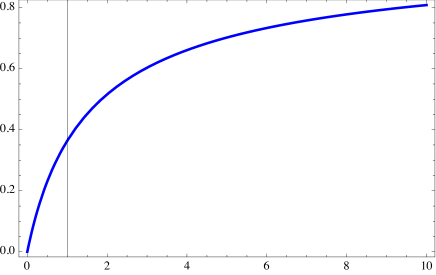
Figure 1: Parentheses of Eq. (6) versus $\eta$ for $0<\eta<10$.

Note that $\lambda_{d}^{-2}(0,\eta)=4\pi^{2}\sigma\Delta_{0}/\hbar c^{2}\propto\sigma T_{c}$, the same scaling as in the dirty limit. Hence, deviations from this scaling are determined by the expression in parentheses. Fig. 1 shows that this expression varies only by a factor of 2 when the scattering parameter $\eta$ changes from 10 to 1, the latter value corresponding to the quite clean situation with $\xi_{0}/\ell=2/\pi=0.64$. This suggests that the dirty limit scaling may work quite well in a broad domain of scattering parameters; even more so visually if one employs log-log plots.

To show this, we express $\lambda_{d}^{-2}(0,\eta)$ and $\eta$ in terms of the product $x=\sigma T_{c}$ in K/$\Omega\,$cm since these units are preferred by experimentalists: Homes

$$\lambda_{d}^{-2}(0,\eta)\,{\rm cm}^{-2}=0.915\times 10^{4}\,x\,$$

$$\eta=\frac{4\pi^{2}e^{2}N(0)v^{2}}{3c^{2}\lambda_{d}^{-2}(0)}=\frac{6.1\times 10^{6}}{x}\,,$$ (7)

Here, $N(0)v^{2}=3n/2m\approx 1.65\times 10^{49}$ CGS for the free electrons is taken as an estimate ($n\approx 10^{22}\,$cm^-3 and $m$ is the free electron mass). With these numbers Eq. (6) generates the curve shown in Fig. 2.

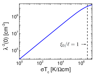
Figure 2: The log-log plot of $\lambda^{-2}\,$cm^-2 versus $x=\sigma T_{c}$ in K/$\Omega\,$cm. The vertical line shows $x$ corresponding to $\xi_{0}/\ell=1$.

The left part of this plot corresponds to large scattering parameters $\eta$, whereas the right one represents the clean situation. The boundary between these extremes is $\xi_{0}/\ell\approx 1$ or $\eta\approx\pi/2$. With the numbers chosen, this corresponds to $\sigma T_{c}\approx 3.9\times 10^{6}\,$K/$\Omega\,$cm. Hence, the figure shows that in a broad range of the variable $\sigma T_{c}$, the behavior of $\lambda^{-2}(0)$ is in fact close to that of the dirty limit. The maximum $\sigma T_{c}=10^{7}\,$K/$\Omega\,$cm of the figure (and of the data collection of Ref. Homes, ) corresponds to $\xi_{0}/\ell\approx 0.2$, i.e., to clean materials. When the material is in the clean limit $\eta\to 0$, the curve of Fig. 2 flattens to approach

$$\lambda^{-2}_{\rm clean}(0)=\frac{8\pi e^{2}N(0)v^{2}}{3c^{2}}=\frac{4\pi e^{2}n}{mc^{2}}\,.$$ (8)

This, however, happens at very large values of $\sigma T_{c}$ out of the range of available data.Homes At the maximum available $\sigma T_{c}=10^{7}\,$K/$\Omega\,$cm the deviation of the curve on the log-log plot of Fig. 2 from the straight line is about 7%.

Thus, qualitatively, “Homes scaling”, shown in Fig. 2 of Ref. Homes, , is well reproduced by the BCS theory and does not necessarily call for exotic constructions for its justification.Zaanen ; Imry ; Erd The oversimplified scheme presented here, of course, can be improved by taking into account anisotropies, variations in densities of states, Fermi velocities, pair breaking, etc. It strongly suggests, however, that the idea of the dirty limit scaling is certainly viable and can be extended to a broad range of scattering parameters. The extensive set of data summarized by the Homes scaling can be considered as yet another confirmation of the BCS theory, if any is still needed.

The author is grateful to S. Bud’ko, P. Canfield, R. Prozorov, J. Clem, V. Taufour, and H. Kim for interest and help. Discussions with C. Homes were welcome and encouraging. The Ames Laboratory is supported by the Department of Energy, Office of Basic Energy Sciences, Division of Materials Sciences and Engineering under Contract No. DE-AC02-07CH11358.

References

- (1) S. V. Dordevic, D. N. Basov, and C. C. Homes, Nature Scientific Reports, 3, 1713 (2013); arXive:1305.0019.
- (2) C. C. Homes, S. V. Dordevic, M. Strongin, D. A. Bonn, R. Liang, W. N. Hardy, S. Komiya, Y. Ando, G. Yu, N. Kaneko, X. Zhao, M. Greven, D. N. Basov, and T. Timusk, Nature (London) 430, 539 (2004).
- (3) J. Zaanen, Nature (London) 430, 512 (2004).
- (4) C. C. Homes, S. V. Dordevic, T. Valla, and M. Strongin, Phys. Rev. B72, 134517 (2005).
- (5) J. L. Tallon, J. R. Cooper, S. H. Naqib, and J. W. Loram, Phys. Rev. B 73, 180504 (2006).
- (6) D. N. Basov and A. V. Chubukov, Nature Physics, 7, 272 (2011).
- (7) Y. Imry, M. Strongin, and C. C. Homes, Phys. Rev. Lett. 109, 067003 (2012).
- (8) J. Erdmenger, P. Kerner, and S. Muller, Journal of High Energy Physics 2012, 1-36 (2012).
- (9) A. A. Abrikosov, L. P. Gor’kov, I. E. Dzyaloshinskii, Methods of Quantum Field Theory in Statistical Physics, Englewood Cliffs, N.J., Prentice-Hall, 1963.
- (10) V. G. Kogan, A. Gurevich, J.H.Cho, D.C.Johnston, Ming Xu, J. R. Thompson, and A. Martynovich, Phys. Rev. B, 54, 12386 (1996).
- (11) R. Prozorov and V. G. Kogan, Reports on Progress in Physics 74, 124505 (2011).