Evolution and excitation conditions of outflows
in high-mass star-forming regions

Abstract

Context. Theoretical models suggest that massive stars form via disk-mediated accretion, in a similar fashion to low-mass stars. In this scenario, bipolar outflows ejected along the disk axis play a fundamental role, and their study can help to characterize the different evolutionary stages involved in the formation of a high-mass star. A recent study toward massive molecular outflows has revealed a decrease of the SiO line intensity as the object evolves.

Aims. The present study aims at characterizing the variation of the molecular outflow properties with time, and at studying the SiO excitation conditions in outflows associated with high-mass young stellar objects (YSOs).

Methods. We used the IRAM 30-m telescope on Pico Veleta (Spain) to map 14 high-mass star-forming regions in the SiO (2–1), SiO (5–4) and HCO⁺ (1–0) lines, which trace the molecular outflow emission. The FTS backend, covering a total frequency range of $\sim$15 GHz, allowed us to simultaneously map several dense gas (e. g., N₂H⁺, C₂H, NH₂D, H¹³CN) and hot core (CH₃CN) tracers. We used the Hi-GAL data to improve the previous spectral energy distributions, and obtain a more accurate dust envelope mass and bolometric luminosity for each source. We calculated the luminosity-to-mass ratio, which is believed to be a good indicator of the evolutionary stage of the YSO.

Results. We detect SiO and HCO⁺ outflow emission in all the fourteen sources, and bipolar structures in six of them. The outflow parameters are similar to those found toward other massive YSOs with luminosities $10^{3}$–$10^{4}$ $L_{\sun}$. We find an increase of the HCO⁺ outflow energetics as the object evolve, and a decrease of the SiO abundance with time, from $10^{-8}$ to $10^{-9}$. The SiO (5–4) to (2–1) line ratio is found to be low at the ambient gas velocity, and increases as we move to red/blue-shifted velocities, indicating that the excitation conditions of the SiO change with the velocity of the gas. In particular, the high-velocity SiO gas component seems to arise from regions with larger densities and/or temperatures, than the SiO emission at the ambient gas velocity.

Conclusions. The properties of the SiO and HCO⁺ outflow emission suggest a scenario in which SiO is largely enhanced in the first evolutionary stages, probably due to strong shocks produced by the protostellar jet. As the object evolves, the power of the jet would decrease and so does the SiO abundance. During this process, however, the material surrounding the protostar would have been been swept up by the jet, and the outflow activity, traced by entrained molecular material (HCO⁺), would increase with time.

Table 1: List of observed sources, and spectral energy distribution parameters

		$\alpha$	$\delta$	$V_{\mathrm{lsr}}$b	$D$		SED fitd			$L_{\mathrm{bol}}$e	$L/M$
#	Sourcea	(J2000)	(J2000)	(km s-1)	(kpc)	IRc	$\beta$	$T_{\mathrm{dust}}$ (K)	$M$ ($M_{\sun}$)	($L_{\sun}$)	($L_{\sun}$ $M_{\sun}$-1)
01	18151$-$1208_1	18:17:58.0	$-$12:07:27.0	$+$33.0	3.0	L	1.7	32	0478	26090	54.6
02	G19.27$+$0.1M2	18:25:52.6	$-$12:04:48.0	$+$26.9	2.4	D	2.5	35	0077	00157	02.0
03	G19.27$+$0.1M1	18:25:58.5	$-$12:03:59.0	$+$26.5	2.4	D	1.3	22	0193	00374	01.9
04	18236$-$1205	18:26:25.4	$-$12:03:51.4	$+$26.5	2.5	L	1.0	29	0935	04507	04.8
05	18264$-$1152	18:29:14.4	$-$11:50:21.3	$+$43.7	3.5	L	1.3	27	1634	11910	07.3
06	G23.60$+$0.0M1	18:34:11.6	$-$08:19:06.0	$+$106.50	6.2	D	2.0	18	1820	05207	02.9
07	18316$-$0602	18:34:20.5	$-$05:59:30.4	$+$42.5	3.1	L	1.2	33	1613	31820	19.7
08	G23.60$+$0.0M2	18:34:21.1	$-$08:18:07.0	$+$53.5	3.9	D	1.9	23	0287	03049	10.6
09	G24.33$+$0.1M1	18:35:07.9	$-$07:35:04.0	$+$113.60	6.7	D	2.2	23	2674	48050	18.0
10	G34.43$+$0.2M1f	18:53:18.0	$+$01:25:23.0	$+$57.9	3.7	D	1.8	26	1369	24050	17.6
11	18507$+$0121	18:53:19.6	$+$01:24:37.1	$+$57.6	3.7	L	1.0	29	3065	14530	04.7
12	G34.43$+$0.2M3	18:53:20.4	$+$01:28:23.0	$+$59.2	3.7	D	1.5	21	0612	01357	02.2
13	19095$+$0930	19:11:54.0	$+$09:35:52.0	$+$43.9	3.3	L	1.6	33	0971	50680	52.2
14	23139$+$5939	23:16:11.1	$+$59:55:30.8	$-$44.5	4.8	L	1.6	30	0972	26040	26.8

• Name of sources starting with numbers (e. g., 18151$-$1208) refer to the IRAS name (Neugebauer et al., 1984).

• Systemic velocity ($V_{\mathrm{LSR}}$) derived from the hyperfine fit to the N₂H⁺ (1–0) and C₂H (1–0) lines (see Sect. 3.1).

• Sources classified as IR-luminous (IRL) or IR-dark (IRD) according to its emission or not at mid-IR wavelengths according to López-Sepulcre et al. (2010).

• Parameters obtained from the single-temperature, modified black body fit to the spectral energy distribution (see Sect. 3.3).

• Bolometric luminosity derived by integrating over the full observed spectral distribution (see Sect. 3.3).

• Observed simultaneously with (in the same map as) 18507$+$0121.

1 Introduction

Establishing an evolutionary sequence for high-mass young stellar objects (YSOs) is one of the hot topics of current star formation research. It has been proposed that high accretion rates (e. g., McKee & Tan, 2003) and/or accretion through massive disks (e. g., Krumholz et al., 2005) can explain the formation of massive stars. Recently, Kuiper et al. (2010, 2011) have demonstrated that stars with masses up to 140 $M_{\sun}$, can be formed via disk-mediated accretion. In this context a fundamental role is played by a bipolar outflow ejected along the disk axis. So far, a number of deeply embedded massive disk/outflow systems (see Cesaroni et al., 2007) have been found, lending support to such models.

Studying the properties of molecular outflows can provide information on the different evolutionary stages during the formation process of a massive star. Beuther & Shepherd (2005) propose an evolutionary sequence for outflows driven by high-mass protostars in which a well-collimated outflow/jet gradually evolves into a wide-angle outflow/wind as the ionizing radiation powered by the central massive stellar object becomes more dominant. However, understanding the outflow population in high-mass star-forming regions is not always easy, due to the high level of clustering in these regions. Many high-mass star-forming regions show evidence for several outflows (e. g., 05358$+$3543: Beuther et al. 2002c, AFGL 5142: Zhang et al. 2007). In such a situation, lack of outflow bipolar signatures is to be expected in clustered star-forming regions, being thus interesting the identification of these bipolar structures.

Most of the observations of massive molecular outflows carried up to date, have focused on the CO and HCO⁺ species, and their isotopologues. These molecules typically trace the low-velocity, extended, entrained gas component of the outflow and, in some cases, appear contaminated by the surrounding (infalling) envelope. Observations of a more reliable jet tracer are thus necessary to better characterize the jet/outflow properties. SiO emission is ideal for this purpose, because its formation is attributed to sputtering or vaporization of Si atoms from grains due to fast shocks (Gusdorf et al., 2008a, b; Guillet et al., 2009), and thus suffers minimal contamination from quiescent or infalling envelopes. Recently, López-Sepulcre et al. (2011) studied the SiO (2–1) and (3–2) line emission toward a sample of 57 high-mass YSOs. These authors found that the intensity of the SiO line becomes fainter for increasing luminosity-to-mass ratio ($L/M$), considered an indicator of the evolutionary stage of YSOs. The variation of the SiO line intensity was interpreted as a decrease in the SiO abundance with time (as proposed by Sakai et al. 2010) and/or a decrease in the jet/outflow mass with time.

With this in mind, we performed SiO map observations toward a sub-sample of the López-Sepulcre et al. (2011) sample, to derive the properties of the SiO molecular outflows and better characterize the variation of SiO with time. We also map the outflow emission in HCO⁺, i. e., a tracer of the most extended and entrained gas, and the dense gas emission in different species such as N₂H⁺ or C₂H. In Sect. 2, we describe the observations and the sample of sources. In Sect. 3 we present the main results derived from the IRAM 30 m observations as well as from the fit of the spectral energy distributions. Finally, in Sect. 4 we discuss our results focusing our analysis on the properties of molecular outflows, and in Sect. 5 we summarize our main results.

2 Observations

The IRAM 30 m telescope (Granada, Spain) was used on March 21–25, 2012 to observe in the On-The-Fly (OTF) mapping mode (project 181-11) a sample (see Table 1) of 14 high-mass YSOs selected from the work of López-Sepulcre et al. (2011). The OTF maps have sizes of $1\arcmin\times 1\arcmin$ and were obtained with the EMIR heterodyne receiver tuned simultaneously at two different frequencies: 91.18 GHz (E090 band) and 222.23 GHz (E230 band). At these frequencies, the telescope delivers an angular resolution, beam efficiency and forward efficiency of $\theta_{\mathrm{HPBW}}$=28″, $B_{\mathrm{eff}}$=0.81 and $F_{\mathrm{eff}}$=0.95 in the E090 band, and $\theta_{\mathrm{HPBW}}$=10″, $B_{\mathrm{eff}}$=0.63 and $F_{\mathrm{eff}}$=0.94 in the E230 band. The FTS spectrometer was set as the spectral backend, resulting in a channel resolution of 195 kHz ($\sim$0.6 km s^-1 at 3 mm, and $\sim$0.2 km s^-1 at 1 mm), and a total bandwidth of $\sim$15 GHz: from 85.78 GHz to 93.56 GHz at 3 mm (band E090) and from 216.79 GHz to 224.57 GHz at 1 mm (band E230). We used the position-switching mode, with an OFF position located at ($-$600″,$+$600″) from the center coordinates listed in Table 1. The maps were scanned both along the right ascension and the declination axes to smear scanning effects on the resulting images. System temperatures typically ranged from 100 K to 250 K, reaching in some cases values as high as $\sim$900 K. The weather conditions during the observations, with zenith opacities of 0.15–0.60 at 230 GHz, were not always appropriate for 1 mm observations, and thus, for several sources the noise at 1 mm is too high to detect molecular species other than the strong ¹³CO and C¹⁸O lines. In Table 2, we list the rms noise levels. The accuracy of the pointing was checked every 1.5 or 2 hours. We reduced the data using the CLASS and GREG programs of the GILDAS software package developed by the IRAM and Observatoire de Grenoble. All the resulting spectra have been smoothed to a resolution of 0.8 km s^-1.

In Table 1, we list the 14 objects mapped with the IRAM 30-m telescope (number identifier and name in Cols. 1 and 2), the equatorial coordinates of the center of the maps (Cols. 3 and 4), the systemic velocity (Col. 5) and the heliocentric distance (Col. 6). In Col. 7, we classify each source as IR-luminous (hereafter IRL) or IR-dark (hereafter IRD) according to its emission or not, respectively, at mid-IR wavelengths (see López-Sepulcre et al., 2010).

3 Results

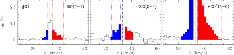
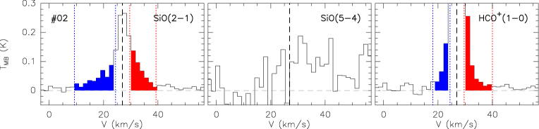
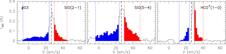
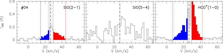
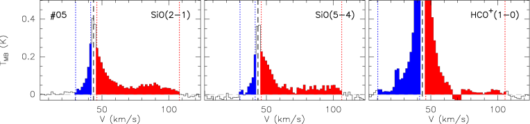
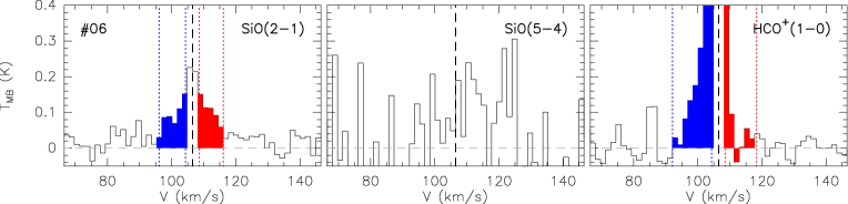
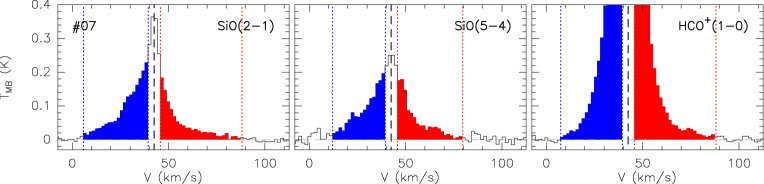
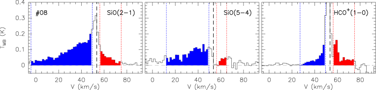
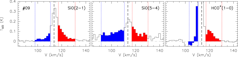
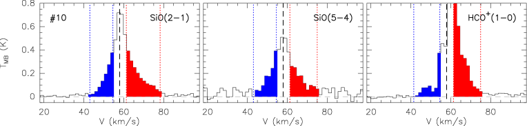
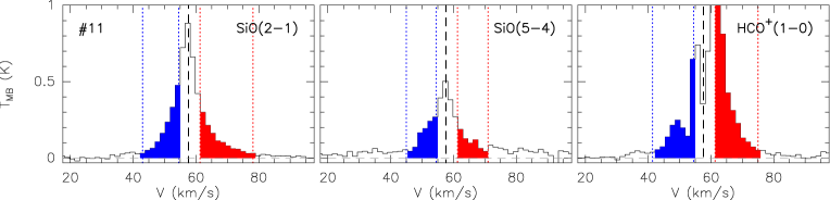
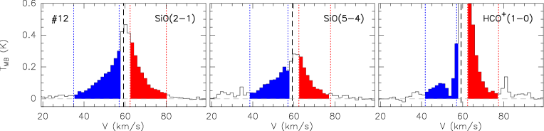
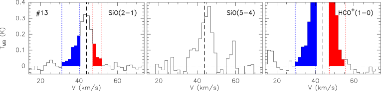
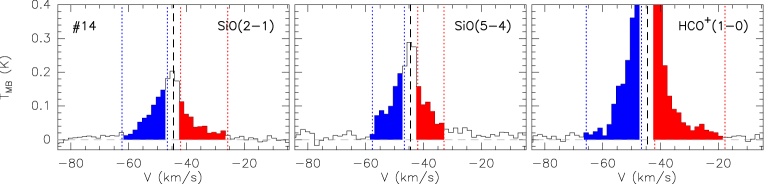
Figure 1: SiO (2–1), SiO (5–4) and HCO⁺ (1–0) spectra (smoothed to a velocity resolution of 1.6 km s^-1). The black dashed vertical line marks the systemic velocity $V_{\mathrm{LSR}}$. The blue and red dotted vertical lines mark the high-velocity outflow wings (see Sect. 3.2), which are also highlighted with colored blue and red histograms. The number of each source (as listed in Table 1) is shown in the top-left corner of the SiO (2–1) panels.

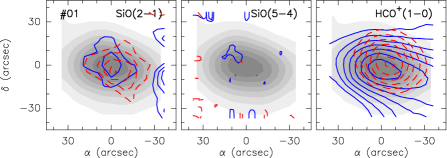
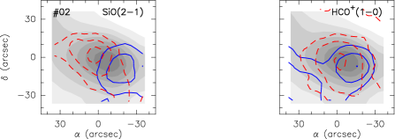
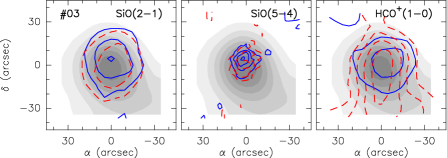
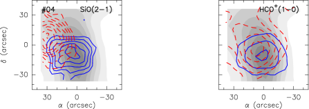
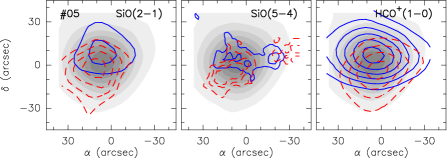
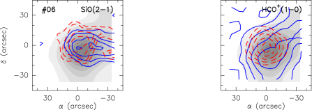
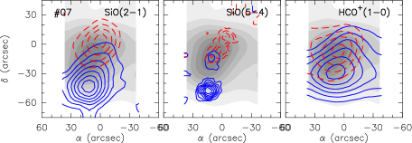
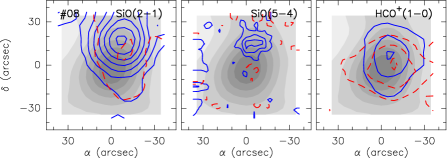
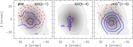
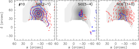
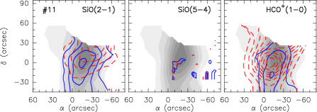
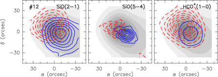
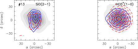
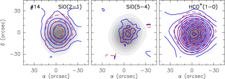
Figure 2: SiO (2–1), SiO (5–4) and HCO⁺ (1–0) outflow maps. Blue- and red-shifted integrated wing emission is shown as blue-solid and red-dashed contours, respectively. The starting and step levels are listed in Table 2. The gray scale corresponds to the N₂H⁺ (1–0) integrated emission as shown in Fig. 11. The number of the region (as listed in Table 1) is indicated in the top-left corner of the SiO (2–1) panel. The x and y axis are the right ascension and declination offsets in arcsec, with the center (0,0) corresponding to the coordinates listed in Table 1. For four sources we do not show the SiO (5–4) panel because we do not detect outflow emission in this line. Note that sources #10 and #11 were observed simultaneously, in the same map.

3.1 Molecular line emission

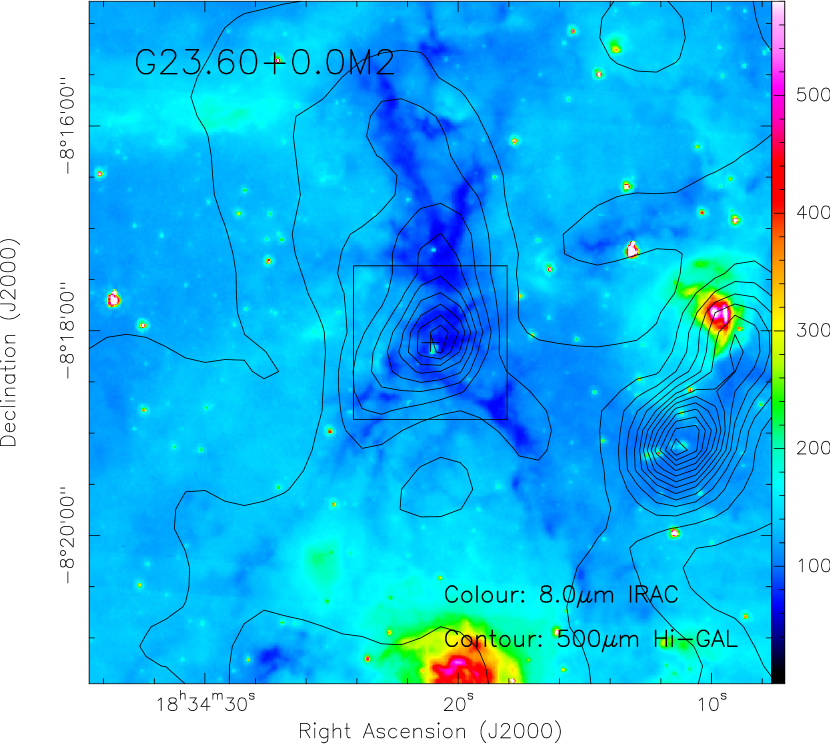
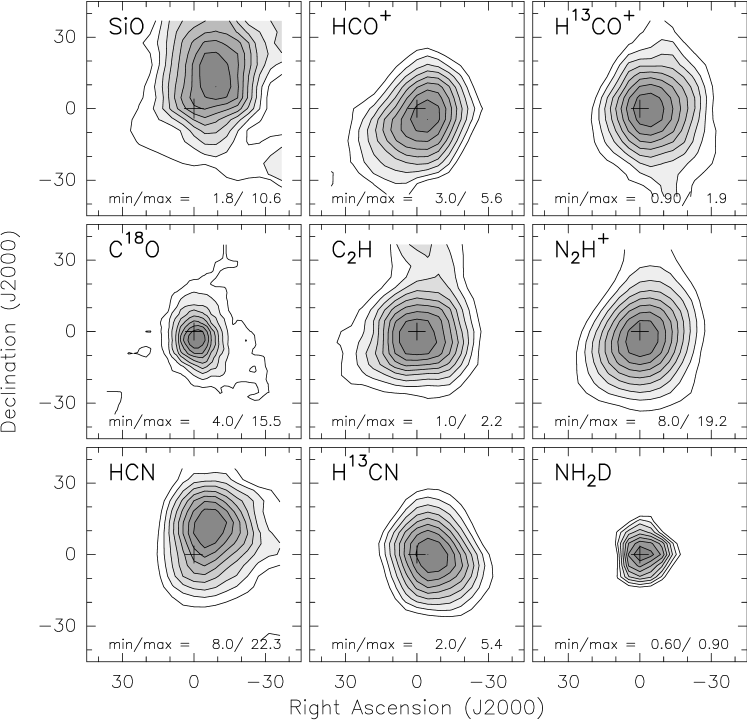
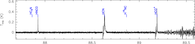
Figure 11: continued, for G23.60$+$0.0 M2.

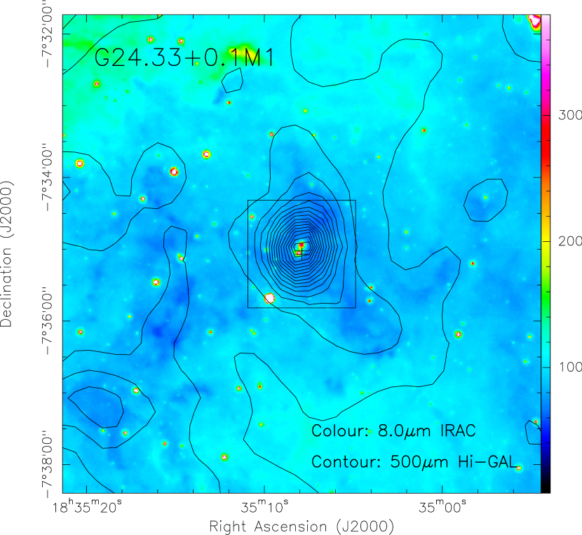
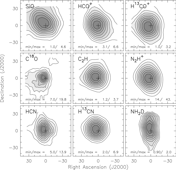
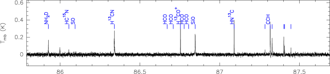
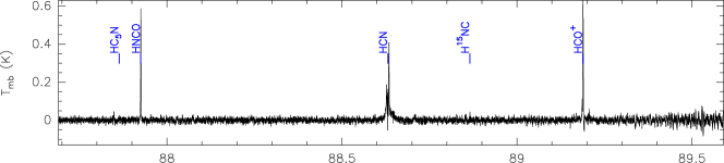
Figure 11: continued, for G24.33$+$0.1 M1.

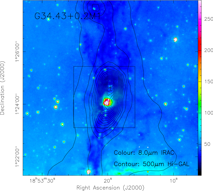
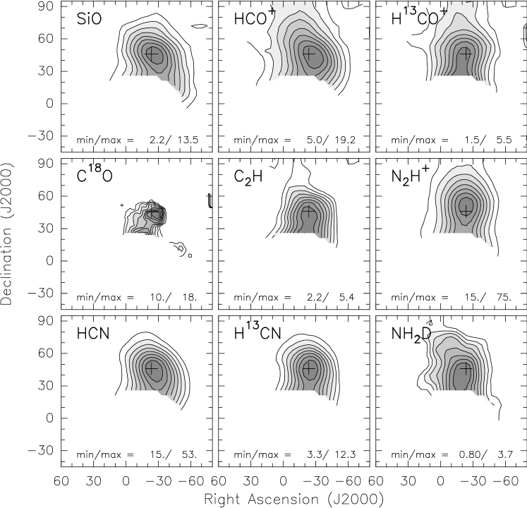
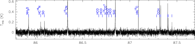
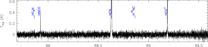
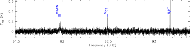
Figure 11: continued, for G34.43$+$0.2 M1.

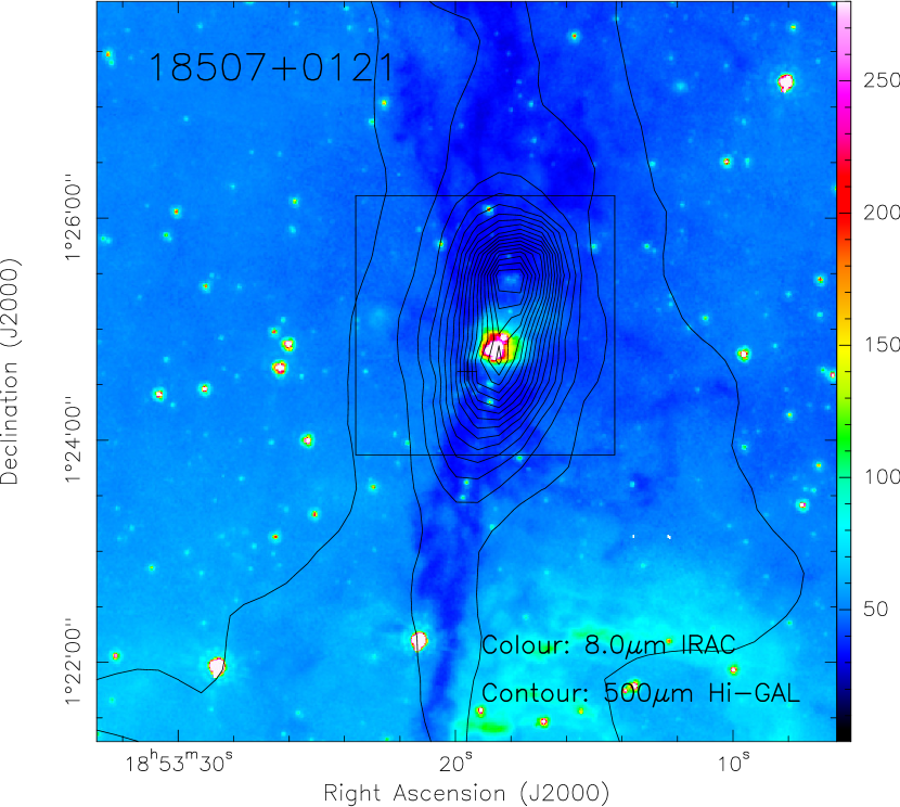
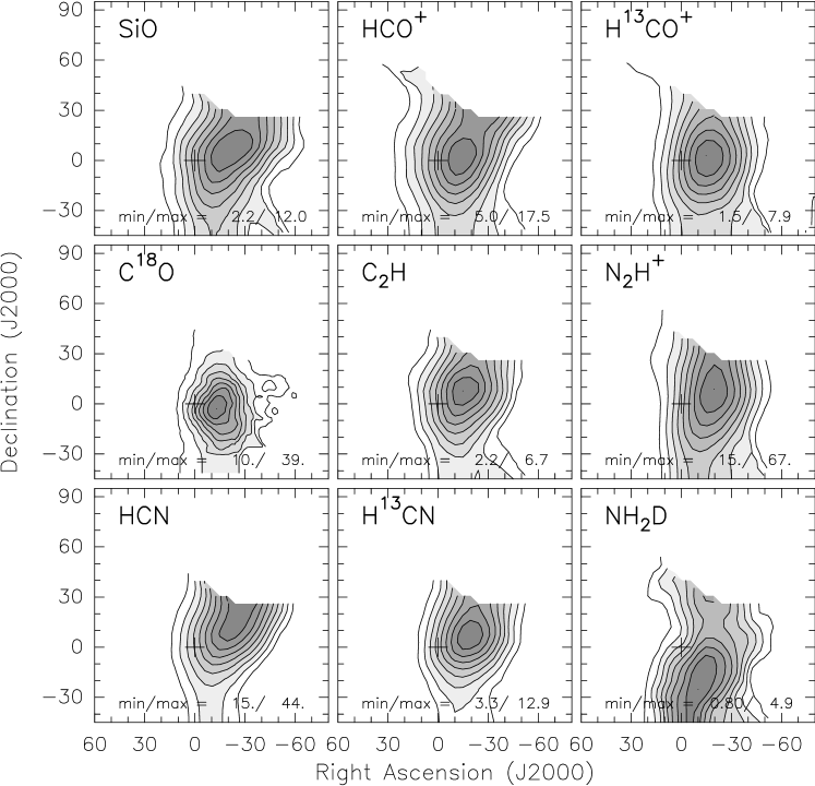
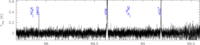
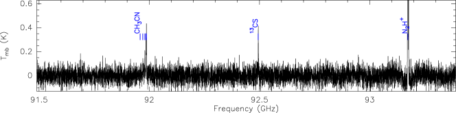
Figure 11: continued, for 18507$+$0121.

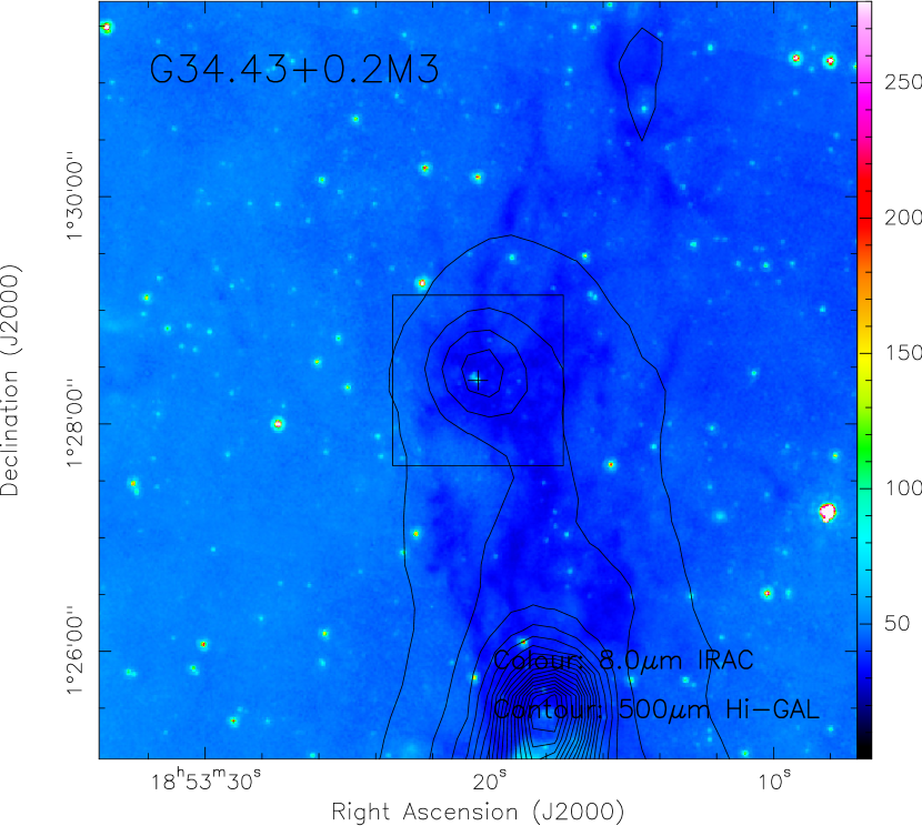
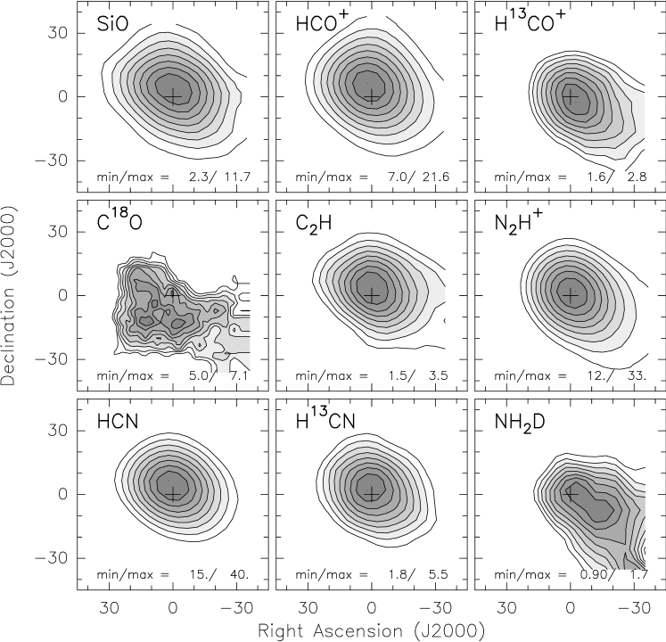
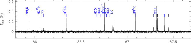
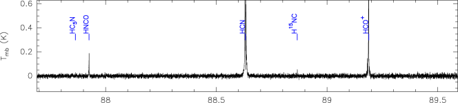
Figure 11: continued, for G34.43$+$0.2 M3.

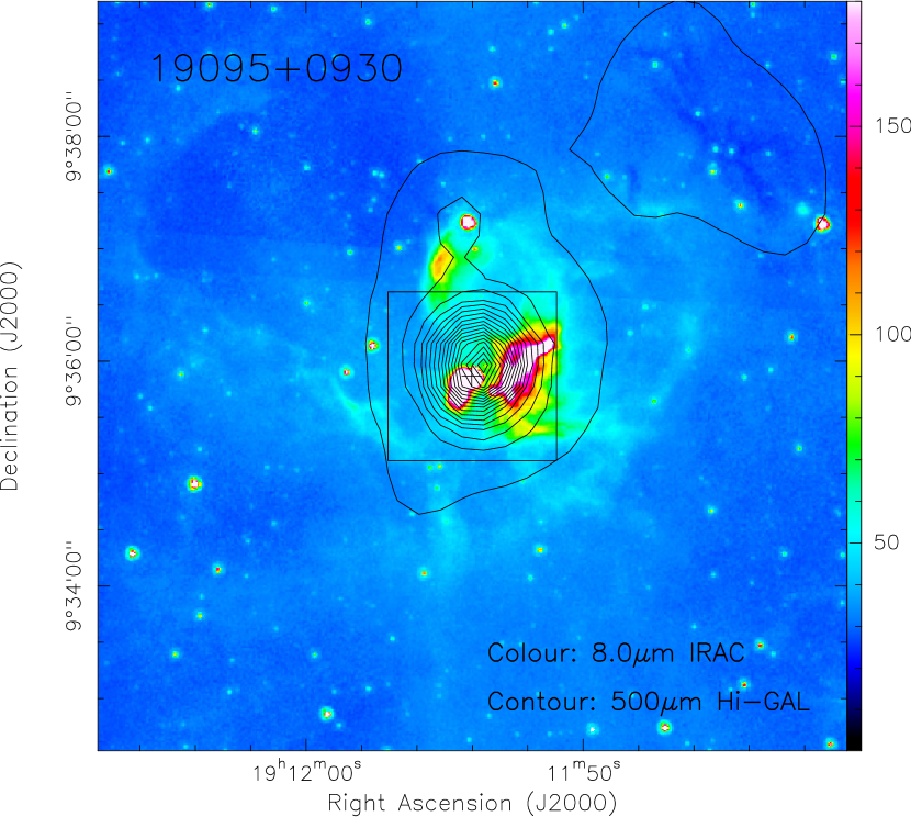
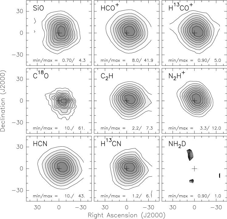
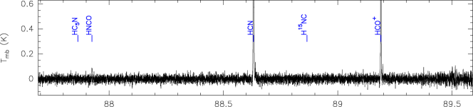
Figure 11: continued, for 19095$+$0930.

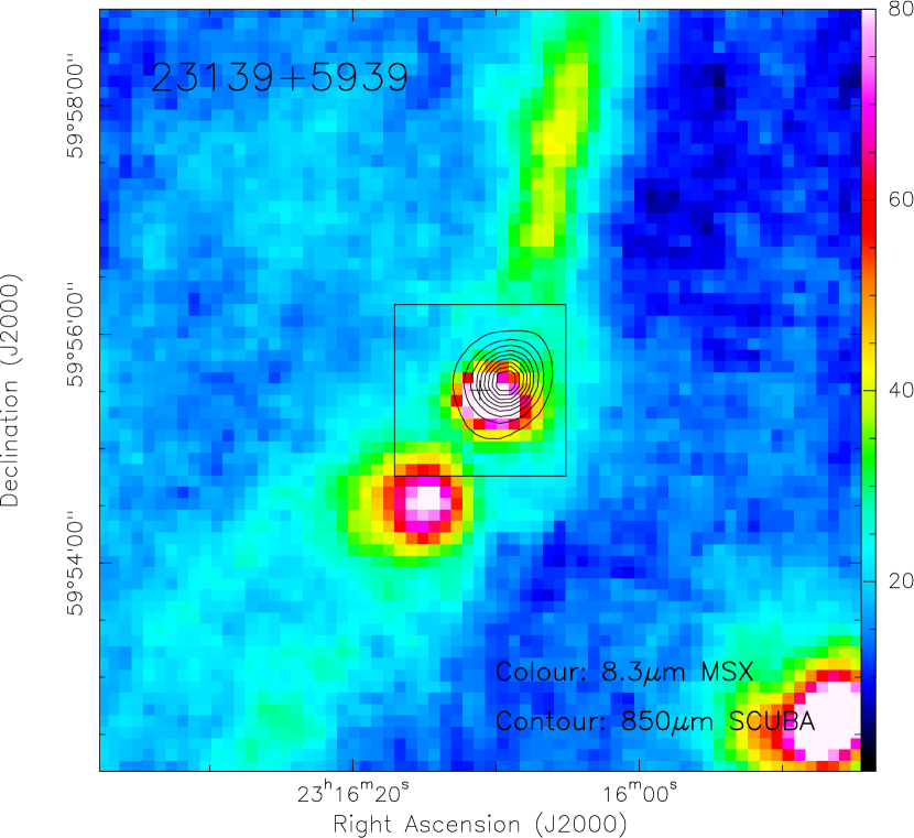
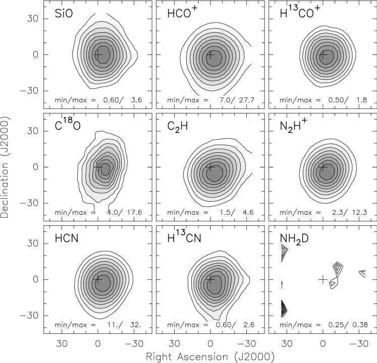
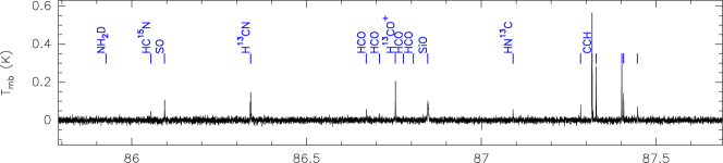
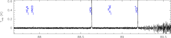
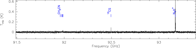
Figure 11: continued, for 23139$+$5939.

The frequency range surveyed at 3 and 1 mm ($\sim$15 GHz in total) allowed us to simultaneously map several molecular transitions, typically found associated with both dense gas and outflow emission. In the bottom panels of Fig. 11, we show the spectra in the 86.48–94.48 GHz frequency range for each source. At 1 mm, the spectra are mainly dominated by noise (due to bad weather conditions, see Sect. 2). We have identified the lines detected with signal-to-noise ratio $\ga$5, which correspond to typical main beam temperatures $\sim$0.1 K. Most of the lines detected toward all the sources of the sample correspond to simple molecules such as N₂H⁺, C₂H, NH₂D or H¹³CN, which are typically found tracing the dense gas in YSOs (e. g., Tafalla et al., 2004; Padovani et al., 2011; Busquet et al., 2011; Fontani et al., 2012), and molecules such as SiO and HCO⁺ typically used to trace the outflow emission (e. g., Tafalla et al., 2010; López-Sepulcre et al., 2010; Codella et al., 2013). For twelve of the fourteen sources, we also detected CH₃CN emission which is a tracer typically found in association with hot cores (e. g., Olmi et al., 1993, 1996; Sánchez-Monge et al., 2010, 2013). Eight of them show emission of high excitation ($K$>2) transitions, which suggests the presence of a dense core with a high temperature. In Table 7, we list the molecular lines detected toward each source.

In the top panels of Fig. 11, we present the zero-order moment (velocity-integrated intensity) maps of outflow tracers (SiO (2–1) and HCO⁺ (1–0)) and ambient velocity dense clump tracers (HCN (1–0), H¹³CN (1–0), H¹³CO⁺ (1–0), C¹⁸O (2–1), C₂H (1–0), N₂H⁺ (1–0) and NH₂D (1,1)), complemented with continuum maps at 8.0 $\mu$m (from Spitzer/IRAC: Infrared Array Camera, Fazio et al. 2004) and 500 $\mu$m (from Herschel/Hi-GAL, Molinari et al. 2010a, b), or alternatively at 8.3 $\mu$m (from MSX: Midcourse Space Experiment, Price et al. 1999) and 850 $\mu$m (from JCMT/SCUBA: Submillimetre Common User Bolometer Array, Di Francesco et al. 2008) when the former images are not available. In the following sections, we will analyze in more detail the molecular lines that can be used to study the properties of the molecular outflows (i. e., SiO and HCO⁺), while a more detailed analysis of the dense gas tracers will be presented in a forthcoming paper. Out of all the molecular lines tracing the dense gas, N₂H⁺ (1–0) and C₂H (1–0) lines are clearly detected in all the regions and have hyperfine structure. We used the HFS method of the CLASS program to take into account the hyperfine structure of the lines. The simultaneous fit to all the hyperfine components provides us with the systemic velocity of the dense gas. The adopted systemic velocity is listed in Col. 5 of Table 1. In addition, from the hyperfine structure fit we obtained a measurement of the line opacity, which allowed us to derive the column density. In Table 8, we list the results of the fit, as well as the excitation temperature, the molecular column density, and the gas mass. The average N₂H⁺ and C₂H column densities are $8.5\times 10^{12}$ cm^-2 and $1.0\times 10^{14}$ cm^-2, respectively.

Table 2: Rms noises and contour levels used in Fig. 2

	SiO (2–1)			SiO (5–4)			HCO+ (1–0)
ID	rmsa	levelsb		rmsa	levelsb		rmsa	levelsb
01	030.7	3(1)		105.4	3(1)		050.8	25(5)
02	043.9	5(3)		320.1	…		053.5	5(3)
03	028.7	5(5)		078.4	3(3)		037.9	5(3)
04	072.7	3(1)		509.6	…		105.8	5(3)
05	031.3	10(5)		078.8	3(3)		085.8	10(5)
06	078.0	3(1)		603.1	…		091.5	5(3)
07	031.1	10(5)		082.1	5(3)		108.0	10(5)
08	033.6	5(5)		103.2	3(3)		049.8	5(3)
09	031.6	5(3)		100.1	5(3)		043.3	5(3)
10	046.5	5(5)		180.5	5(3)		089.5	5(3)
11	046.8	5(5)		179.7	5(3)		089.8	5(3)
12	030.9	10(5)		080.5	5(3)		042.2	10(5)
13	064.7	3(1)		275.4	…		095.2	5(3)
14	028.1	3(3)		068.9	3(3)		046.0	5(3)

• Rms noise level in mK per 0.8 km s^-1 channel.

• Contour levels used in Fig. 2. The first number corresponds to the first contour in terms of $\sigma$, and the number in parenthesis indicates the step level used. The value of $\sigma$ has been calculated from the rms noise per channel, taking into account the velocity range covered to obtain the integrated blue- and red-shifted emission (Tables 3–5).

3.2 Molecular outflow detections

We have assessed the presence of molecular outflows by searching for high-velocity wings in the SiO (2–1), SiO (5–4), and HCO⁺ (1–0) spectra averaged over the area of the 50% contour level in the integrated intensity maps shown in Fig. 11. In Fig. 1, we present the spectra of these three outflow tracers for all the sources in the sample. We detect high-velocity wings in SiO (2–1) and HCO⁺ (1–0) in all the sources, confirming the presence of outflows in these regions as previously reported by López-Sepulcre et al. (2010, 2011). Note that for a few regions (e. g., G19.27$+$0.1 M2, G23.60$+$0.0 M1), the bad weather conditions during observations resulted in noisy SiO (5–4) spectra (cf. noises listed in Table 2) that prevented detection of high-velocity wings in SiO (5–4). The new HCO⁺ (1–0) spectra have 1$\sigma$ rms noises ($\sim$70 mK) a few times better than the previous observations of López-Sepulcre et al. (2010, $\sim$480 mK), improving the detection of faint emission at high velocities.

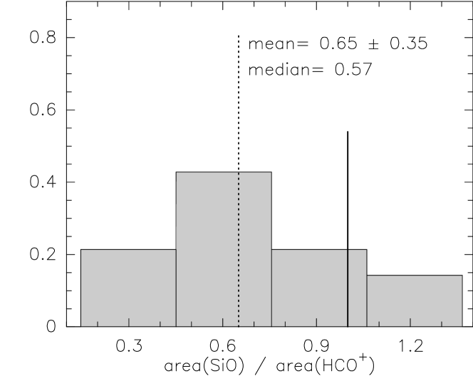
Figure 3: Distribution of the SiO (2–1) to HCO⁺ (1–0) area ratio for the outflow emission. The solid vertical line corresponds to the equality (i. e., equal sizes for the SiO and HCO⁺ outflow lobes). The dotted vertical line marks the mean value of the distribution. The mean ($\pm$ standard deviation) and median values are shown in the panel. The total number of sources is 14.

The red and blue high-velocity wings are shown in each spectra of Fig. 1. For each source with line wings, we compared the spectra of the outflow tracers with those from dense gas tracers such as C₂H, N₂H⁺ and H¹³CO⁺ and, following the approach of López-Sepulcre et al. (2009), we defined the low-velocity limits where the line intensities of the C₂H ($1_{2,2}$–$0_{1,1}$), N₂H⁺ ($1_{0}$–$0_{1}$) and H¹³CO⁺ (1–0) transitions fall below 2$\sigma$. In a few cases where also these lines display non-Gaussian extended wings, the beginning of the departure from a Gaussian fit on the observed spectra has been chosen as low-velocity limits for the outflow. The high-velocity limits have been chosen where the line intensity of the outflow tracers falls below 2$\sigma$. After inspection of the channel maps, these limits were in some cases slightly modified, based on the observed spatial distribution of the blue- and red-shifted emission. The resulting outflow velocity ranges ($\Delta V_{\mathrm{blue}}$ and $\Delta V_{\mathrm{red}}$) are listed in Cols. 4 and 5 of Tables 3, 4 and 5, and have been used to obtain the outflow maps in Fig. 2, as well as to compute the outflow parameters (see Sect. 4.1).

The outflow maps are presented in Fig. 2, where the blue and red wing emission of SiO (2–1), SiO (5–4) and HCO⁺ (1–0) lines (solid-blue and red-dashed contours, respectively) are superimposed on the N₂H⁺ (1–0) integrated emission (gray scale). We identify a bipolar structure in the outflow emission for six regions: G19.27$+$0.1M2, 18236$-$1205, 18264$-$1152, 18316$-$0602, G24.33$+$0.1M1, and G34.43$+$0.2M3. For all these sources, but one (18236$-$1205), the geometrical center of the two outflow lobes is close to the peak of the dense clump (see gray scale tracing the N₂H⁺ emission in Fig. 2). For a few sources, and despite the presence of extended high-velocity wings, we do not find bipolar morphology in the maps (e. g., 23139$+$5939). This fact suggests that the outflow is directed close to the line of sight, or that a more complex structure (with multiple outflows) produces the high-velocity emission that we detect. Higher angular resolution observations are necessary to study the presence of multiple outflows in some of these regions. In general, the SiO and HCO⁺ profiles and spatial distributions are similar though in detail different. The extent in velocity of the profiles is similar, and both species have the same orientation in the bipolar cases. However, the HCO⁺ spatial distribution is more extended than the SiO one. This is shown in Fig. 3, where we plot the distribution of the SiO to HCO⁺ area ratio. The area is calculated as the sum of the red and blue outflow lobe areas, determined by the deconvolved sizes listed in Col. 6 of Tables 3 and 5. The mean and median values of the distribution are 0.65 and 0.57. This supports the idea that SiO is associated with a more collimated agent (primary jet, although not resolved in our observations) and that HCO⁺ is associated with extended entrained gas, as found in different star-forming regions with higher angular resolutions (e. g., Cesaroni et al., 1999).

Table 3: SiO (2–1) molecular outflows: velocity ranges of the wings, lobe sizes, outflow energetics and kinematics

	$V_{\mathrm{LSR}}$	$\Delta V_{\mathrm{blue}}$	$\Delta V_{\mathrm{red}}$	$V_{\mathrm{max-b/r}}$a	sizeblue/redb	$M_{\mathrm{out}}$	$p_{\mathrm{out}}$	$E_{\mathrm{out}}$	$t_{\mathrm{kin}}$
ID	(km s-1)	(km s-1)	(km s-1)	(km s-1)	(pc)	($M_{\sun}$)	($M_{\sun}$ km s-1)	(1046 erg)	(104 yr)
01	0$+$33.0	[$+$26.9 ;$+$31.4]	[$+$34.9 ;$+$43.7]	06.1  / 10.7	0.31 / 0.20	009.7	036	00.18	3.0
02	0$+$26.9	0[$+$9.3 ;$+$24.4]	[$+$29.6 ;$+$39.3]	17.6 / 12.4	0.19 / 0.28	003.8	026	00.23	1.5
03	0$+$26.5	0[$-$6.6 ;$+$24.0]	[$+$30.0 ;$+$44.9]	33.1 / 18.4	0.23 / 0.18	013.0	140	02.30	0.9
04	0$+$26.5	[$+$14.5 ;$+$24.6]	[$+$29.4 ;$+$44.1]	12.0 / 17.6	0.27 / 0.36	035.0	280	02.80	2.2
05	0$+$43.7	[$+$30.3 ;$+$41.6]	0[$+$46.2 ;$+$107.9]	13.4 / 64.2	0.35 / 0.51	110.0	21300	75.00	2.1
06	$+$106.5	0[$+$96.1 ;$+$104.3]	[$+$108.6 ;$+$116.1]	10.4 / 09.6	0.66 / 0.73	036.0	210	01.40	6.8
07	0$+$42.5	0[$+$5.9 ;$+$39.5]	[$+$45.8 ;$+$88.1]	36.6 / 45.6	0.33 / 0.37	103.0	14000	27.00	0.8
08	0$+$53.5	0[$-$4.2 ;$+$49.6]	[$+$56.3 ;$+$75.0]	57.7 / 21.5	0.53 / 0.47	024.0	470	14.00	1.6
09	$+$113.6	0[$+$97.8 ;$+$110.7]	[$+$117.2 ;$+$131.2]	15.8 / 17.6	1.14 / 0.97	054.0	420	04.10	6.2
10	0$+$57.9	[$+$43.0 ;$+$54.5]	[$+$61.3 ;$+$78.2]	14.9 / 20.3	0.48 / 0.35	076.0	630	06.50	2.3
11	0$+$57.6	[$+$43.0 ;$+$54.5]	[$+$61.3 ;$+$78.2]	14.6 / 20.6	0.54 / 0.82	099.0	750	07.10	4.0
12	0$+$59.2	[$+$35.0 ;$+$57.1]	[$+$62.4 ;$+$80.0]	24.2 / 20.8	0.38 / 0.42	050.0	440	05.10	1.7
13	0$+$43.9	[$+$31.1 ;$+$40.2]	[$+$47.2 ;$+$51.9]	12.8 / 08.0	0.32 / 0.19	008.5	055	00.41	2.7
14	0$-$44.5	[$-$62.3 ;$-$46.6]	[$-$42.0 ;$-$25.7]	17.8 / 18.8	0.17 / 0.38	063.0	450	04.30	1.5

• Maximum outflow velocity for the blue and red lobes, respectively, calculated as the difference between the high-velocity limit of the outflow velocity range, $\Delta V$, and the systemic velocity, $V_{\mathrm{LSR}}$.

• Deconvolved size of the blue and red outflow lobes, respectively.

Table 4: SiO (5–4) molecular outflows: velocity ranges of the wings, lobe sizes, outflow energetics and kinematics

	$V_{\mathrm{LSR}}$	$\Delta V_{\mathrm{blue}}$	$\Delta V_{\mathrm{red}}$	$V_{\mathrm{max-b/r}}$a	sizeblue/redb	$M_{\mathrm{out}}$	$p_{\mathrm{out}}$	$E_{\mathrm{out}}$	$t_{\mathrm{kin}}$
ID	(km s-1)	(km s-1)	(km s-1)	(km s-1)	(pc)	($M_{\sun}$)	($M_{\sun}$ km s-1)	(1046 erg)	(104 yr)
01	0$+$33.0	[$+$24.5 ;$+$31.4]	[$+$34.9 ;$+$40.5]	08.5 / 07.5	0.27 / 0.37	002.4	011	000.060	3.6
02	0$+$26.9	…	…	…	…	…	…	…	…
03	0$+$26.5	0[$-$3.7 ;$+$24.0]	[$+$30.0 ;$+$48.3]	30.2 / 21.8	0.12 / 0.07	004.9	054	00.83	0.4
04	0$+$26.5	…	…	…	…	…	…	…	…
05	0$+$43.7	[$+$30.3 ;$+$41.6]	0[$+$46.2 ;$+$106.3]	13.4 / 62.6	0.28 / 0.30	021.0	440	16.00	1.3
06	$+$106.5	…	…	…	…	…	…	…	…
07	0$+$42.5	[$+$12.1 ;$+$39.5]	[$+$45.8 ;$+$79.7]	30.4 / 37.2	0.32 / 0.15	030.0	370	06.30	0.7
08	0$+$53.5	[$+$12.2 ;$+$49.6]	[$+$56.3 ;$+$65.2]	41.3 / 11.7	0.12 / 0.23	004.2	078	01.90	0.8
09	$+$113.6	0[$+$91.4 ;$+$110.7]	[$+$117.2 ;$+$130.4]	22.2 / 16.8	0.40 / 0.46	035.0	370	04.80	2.2
10	0$+$57.9	[$+$43.0 ;$+$54.5]	[$+$61.3 ;$+$75.0]	14.9 / 17.1	0.25 / 0.18	015.0	120	01.10	1.3
11	0$+$57.6	[$+$45.0 ;$+$54.5]	[$+$61.3 ;$+$71.0]	12.6 / 13.4	0.42 / 0.46	011.0	079	00.64	3.3
12	0$+$59.2	[$+$38.6 ;$+$57.1]	[$+$62.4 ;$+$77.8]	20.6 / 18.6	0.28 / 0.21	016.0	130	01.40	1.2
13	0$+$43.9	…	…	…	…	…	…	…	…
14	0$-$44.5	[$-$57.7 ;$-$46.6]	[$-$42.0 ;$-$32.9]	13.2 / 11.6	0.25 / 0.34	020.0	120	00.89	2.3

• Maximum outflow velocity for blue and red lobes (as in Table 3).

• Deconvolved size of the blue and red outflow lobes, respectively.

Table 5: HCO⁺ (1–0) molecular outflows: velocity ranges of the wings, lobe sizes, outflow energetics and kinematics

	$V_{\mathrm{LSR}}$	$\Delta V_{\mathrm{blue}}$	$\Delta V_{\mathrm{red}}$	$V_{\mathrm{max-b/r}}$a	sizeblue/redb	$M_{\mathrm{out}}$	$p_{\mathrm{out}}$	$E_{\mathrm{out}}$	$t_{\mathrm{kin}}$
ID	(km s-1)	(km s-1)	(km s-1)	(km s-1)	(pc)	($M_{\sun}$)	($M_{\sun}$ km s-1)	(1046 erg)	(104 yr)
01	$+$33.0	[$+$22.1 ;$+$31.4]	[$+$34.9 ;$+$53.3]	10.9 / 20.3	0.48 / 0.84	037.0	110	00.57	4.9
02	$+$26.9	[$+$18.1 ;$+$24.4]	[$+$29.6 ;$+$40.0]	08.8 / 13.1	0.37 / 0.28	000.7	003	000.016	2.9
03	$+$26.5	[$+$12.1 ;$+$24.0]	[$+$30.0 ;$+$40.1]	14.4 / 13.6	0.45 / 0.32	001.6	009	000.056	2.7
04	$+$26.5	0[$+$7.3 ;$+$24.6]	[$+$29.4 ;$+$42.5]	19.2 / 16.0	0.46 / 0.36	010.0	065	00.53	2.3
05	$+$43.7	[$+$10.3 ;$+$41.6]	0[$+$46.2 ;$+$105.5]	33.4 / 61.8	0.47 / 0.59	066.0	440	06.80	1.2
06	$+$106.50	0[$+$92.1 ;$+$104.3]	[$+$108.6 ;$+$118.3]	14.4 / 11.8	0.15 / 1.44	057.0	230	01.20	5.5
07	$+$42.5	0[$+$7.5 ;$+$39.5]	[$+$45.8 ;$+$88.1]	35.0 / 45.6	0.58 / 0.75	103.0	930	13.00	1.7
08	$+$53.5	[$+$27.2 ;$+$49.6]	[$+$56.3 ;$+$75.0]	26.3 / 21.5	0.60 / 0.45	005.9	057	00.74	2.2
09	$+$113.60	[$+$103.2 ;$+$110.7]	[$+$117.2 ;$+$130.4]	10.4 / 16.8	0.91 / 0.90	016.0	089	00.64	6.9
10	$+$57.9	[$+$41.4 ;$+$54.5]	[$+$61.3 ;$+$75.0]	16.5 / 17.1	0.64 / 0.56	022.0	150	01.20	3.5
11	$+$57.6	[$+$41.4 ;$+$54.5]	[$+$61.3 ;$+$75.0]	16.2 / 17.4	0.64 / 0.81	032.0	230	01.90	4.3
12	$+$59.2	[$+$41.8 ;$+$57.1]	[$+$62.4 ;$+$77.4]	17.4 / 18.2	0.41 / 0.35	020.0	130	01.10	2.1
13	$+$43.9	[$+$29.5 ;$+$40.2]	[$+$47.2 ;$+$55.8]	14.4 / 11.9	0.29 / 0.26	018.0	089	00.51	2.1
14	$-$44.5	[$-$65.7 ;$-$46.6]	[$-$42.0 ;$-$17.7]	21.2 / 26.8	0.39 / 0.47	037.0	210	01.80	1.8

• Maximum outflow velocity for blue and red lobes (as in Table 3).

• Deconvolved size of the blue and red outflow lobes, respectively.

3.3 Spectral energy distributions

The spectral energy distributions (SEDs) of the sources in this sample were built by López-Sepulcre et al. (2011), with continuum data at different wavelengths (ranging from mid-IR to 1.2 mm) collected from different telescopes and instruments. In this work we improve the SED of each source by complementing the previous data with the Herschel infrared Galactic Plane Survey (Hi-GAL, Molinari et al., 2010a, b) data at 500, 350, 250, 160 and 70 $\mu$m. Compact source detection and extraction were performed with CuTEx (Elia et al., 2010; Molinari et al., 2011) in each of the five Hi-GAL maps separately. In Table 9, we list the continuum fluxes at different wavelengths for each source. The new Hi-GAL data represents a dramatic improvement to the SED, in particular for four sources with no previous data at far-IR/sub-millimeter wavelengths.

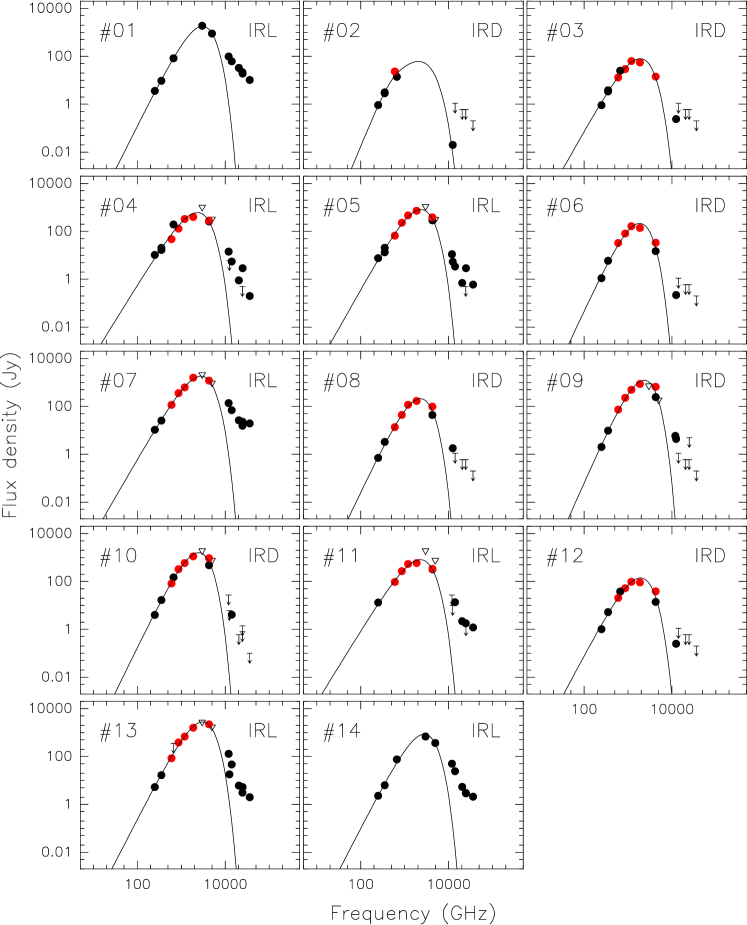
Figure 12: .Spectral energy distributions for the 14 sources listed in Table 1. Black dots correspond to measured continuum fluxes in the range 8 $\mu$m to 1.2 mm (see Table 9), while the crosses correspond to upper limits. Red dots correspond to the new Hi-GAL data (Molinari et al. 2010a, b). White triangles correspond to IRAS fluxes at 60 $\mu$m and 100 $\mu$m not considered in the SED fitting when there is available Hi-GAL data. The solid curve represents the best fit to the data points with wavelengths $\geq 60$ $\mu$m (see Sect. 3.3).

We have fitted the SEDs with a single-temperature, modified black body function, given by $F_{\nu}(T)=\Omega_{\mathrm{S}}\,B_{\nu}(T)\,(1-e^{-\tau_{\nu}})$, where $F_{\nu}(T)$ is the flux at frequency $\nu$, $\Omega_{\mathrm{S}}$ is the solid angle subtended by the source, $B_{\nu}(T)$ is the black body brightness, and $\tau_{\nu}=\tau_{0}\,(\nu/\nu_{0})^{\beta}$ is the frequency-dependent optical depth, with $\kappa_{0}=0.005$ cm² g^-1 at $\nu_{0}=230.6$ GHz (Kramer et al., 2003), assuming a gas-to-dust mass ratio of 100. The best fit was obtained by varying $\beta$ in the range 1.0–2.5, the temperature in the range 10–100 K, and the mass in the range 0.1–10000 $M_{\sun}$, and minimizing the expression $\sum_{\mathrm{i}}(F_{\nu\,\mathrm{i}}^{\mathrm{obs}}-F_{\nu\,\mathrm{i}}^{\mathrm{model}})^{2}$. We aim at determining the properties (mass and temperature) of the dust envelope associated with the massive protostars, which dominates the emission from far-infrared to millimeter wavelengths. Thus, for our best fit calculations, we used only the fluxes at wavelengths $\geq 60$ $\mu$m (i. e., $\nu\leq 5000$ GHz). This permits us to avoid the contribution of a potential, warmer component not associated with the dust envelope, and dominant at shorter wavelengths (see the excess at $\lambda\leq 60$ $\mu$m for some sources in Fig. 12). The best-fit parameters are listed in Cols. 8–10 of Table 1. The bolometric luminosity, listed in Col. 11, has been derived by integrating over the full observed spectral distribution (considering also the emission from the warmer component), $L_{\mathrm{bol}}=4\pi D^{2}\int{F_{\nu}^{\mathrm{obs}}\,d\nu}$, where $D$ is the heliocentric distance to the source. The median dust envelope mass and bolometric luminosity of our sample are 970 $M_{\sun}$ and 13000 $L_{\sun}$, respectively. The masses and luminosities of our sources are in the range 300–3000 $M_{\sun}$ and $10^{3.0}$–$10^{4.5}$ $L_{\sun}$, but for G19.27$+$0.1M1 and G19.27$+$0.1M1. These two sources have luminosities $\sim$$10^{2}$ $L_{\sun}$ and masses of $\sim$100 $M_{\sun}$, about one order of magnitude below the median values. We considered whether the real distance of these sources is the far (13 kpc) rather than the adopted near kinematic (2.4 kpc) distance. However, since these two sources belong to an infrared dark cloud (e. g., Rathborne et al., 2006), it seems improbable that they are located at such a large distance. Probably, these two clumps will produce intermediate-mass stars rather than high-mass stars. We note that for a few sources we obtain low values of $\beta$ (in the range 1.0–1.3), which may be a consequence of assuming an isothermal fit. Finally, in the last column of Table 1, we indicate the luminosity-to-mass ratio, $L/M$, which is believed to be a good indicator of the evolutionary state of the YSO both for the low-mass (e. g., Saraceno et al., 1996) and high-mass (e. g., Molinari et al., 2008) regimes.

Table 6: SiO temperatures and abundances

ID	$T$ (K)a	X(SiO)clumpb	X(SiO)${}_{\mathrm{HCO^{+}}}$c	ratiod
01	18.7	$0.26\times 10^{-9}$	0$0.07\times 10^{-9}$	3.80
02	10.0	$3.82\times 10^{-9}$	$20.22\times 10^{-9}$	0.19
03	13.0	$1.59\times 10^{-9}$	$12.62\times 10^{-9}$	0.13
04	10.0	$0.59\times 10^{-9}$	0$2.03\times 10^{-9}$	0.29
05	15.1	$1.31\times 10^{-9}$	0$2.17\times 10^{-9}$	0.60
06	10.0	$1.36\times 10^{-9}$	0$0.85\times 10^{-9}$	1.60
07	12.7	$2.13\times 10^{-9}$	0$2.12\times 10^{-9}$	1.01
08	09.6	$7.32\times 10^{-9}$	$29.95\times 10^{-9}$	0.24
09	11.0	$2.09\times 10^{-9}$	0$7.19\times 10^{-9}$	0.29
10	12.9	$2.62\times 10^{-9}$	0$9.20\times 10^{-9}$	0.29
11	13.0	$1.69\times 10^{-9}$	0$5.15\times 10^{-9}$	0.33
12	11.7	$4.19\times 10^{-9}$	$10.64\times 10^{-9}$	0.39
13	10.0	$0.47\times 10^{-9}$	0$0.22\times 10^{-9}$	2.08
14	13.6	$1.07\times 10^{-9}$	0$1.79\times 10^{-9}$	0.60

• Temperature used to derive the outflow parameters (see Sect. 4.1), which has been computed as the rotational temperature derived from the SiO (2–1) and (5–4) lines, except for those sources with no detection of the SiO (5–4) for which we assumed a value of 10 K.

• SiO abundance derived from the ratio between the number of SiO particles over the clump and the corresponding H₂ gas mass, which was obtained from the relation between the outflow mass and the mass of the clump $M_{\mathrm{out}}=0.3\,M_{\mathrm{clump}}^{0.8}$ (e. g., Beuther et al., 2002b; López-Sepulcre et al., 2010).

• SiO abundance derived from the ratio of the SiO and HCO⁺ column densities, and assuming a fixed HCO⁺ abundance of $5\times 10^{-9}$ (Irvine et al., 1987; Tafalla et al., 2010; Busquet et al., 2011; Tafalla & Hacar, 2013).

• X(SiO)_clump to X(SiO)${}_{\mathrm{HCO^{+}}}$ ratio.

4 Analysis and Discussion

4.1 Derivation of outflow parameters

We used the procedure described in Eqs. (4)–(6) of López-Sepulcre et al. (2009) to derive the outflow mass ($M_{\mathrm{out}}$), momentum ($p_{\mathrm{out}}$) and mechanical energy ($E_{\mathrm{out}}$) of the SiO and HCO⁺ molecular outflows. These quantities have been calculated from the emission integrated inside the outflow velocity limits ($\Delta V_{\mathrm{blue}}$ and $\Delta V_{\mathrm{red}}$) and, spatially, over the area defined by the 5$\sigma$ contour level of the corresponding outflow lobe (Fig. 2). In the calculations, the temperature for HCO⁺ was fixed to 10 K (the outflow parameters increase by a factor 1.5 and 2 for temperature of 20 K and 30 K, respectively). For SiO, we calculated the rotation temperature from the intensity ratio of the SiO (2–1) and (5–4) lines for the ten sources in which both lines are detected, while we considered a fixed value of 10 K for the remaining four sources. The computed values are listed in Table 6. The mean temperature for these ten sources is $\sim$13 K, which is similar to the assumed temperature of 10 K for the other sources. We assumed optically thin emission for both species. This is a common assumption for SiO outflows observed with single-dish telescopes (i. e., angular resolutions $\ga$10″), and seems reasonable for the high-velocity component of our HCO⁺ outflows, since no H¹³CO⁺ (1–0) line emission is detected at high velocities (see e. g., Fig. 4).

For the abundances, we used a fixed value of $5\times 10^{-9}$ for HCO⁺. Several works (e. g., Irvine et al., 1987; Tafalla et al., 2010; Busquet et al., 2011; Tafalla & Hacar, 2013) report, from studies in different star-forming regions, an HCO⁺ abundance in the range $1$-$9\times 10^{-9}$, with no large enhancements when comparing the outflow gas with the dense core. In contrast, the abundance of SiO has been found to vary by several orders of magnitude, with values ranging from $10^{-12}$ to $10^{-7}$ (e. g., Ziurys et al., 1989; Bachiller & Perez Gutierrez, 1997; Garay et al., 1998; Codella et al., 2005; Nisini et al., 2007). For our sources, we refrained from assuming a given SiO abundance and estimated it using two approaches. First, we derived the SiO abundance from the ratio between the number of SiO particles over the clump and the corresponding H₂ gas mass. The former was derived from the SiO emission integrated in all the velocity range and, spatially, over the clump size, using the excitation temperatures listed in Table 6. The latter was obtained from the relation between the outflow mass and the mass of the clump (listed in Table 1): $M_{\mathrm{out}}=0.3\,M_{\mathrm{clump}}^{0.8}$ (e. g., Beuther et al., 2002b; López-Sepulcre et al., 2009). The SiO abundances derived with this method are listed in Col. 3 of Table 6. In a second approach, we derived the SiO abundance by taking the ratio of the SiO and HCO⁺ column densities in the high-velocity regime, and assuming a standard HCO⁺ abundance of $5\times 10^{-9}$. We did not consider the emission at systemic velocities to exclude the HCO⁺ emission from the bulk gas. A caveat is that although HCO⁺ seems to have quite a stable abundance, some studies have revealed some enhancement of HCO⁺ in high velocity bullets (e. g., Tafalla et al., 2010; Pacheco, 2012). The abundances obtained with this method are listed in Col. 4 of Table 6. The X(SiO)_clump to X(SiO)${}_{\mathrm{HCO^{+}}}$ ratio varies from 4 to 0.1, with a median of 0.36 (cf. Col. 5 of Table 6). The SiO abundance in our outflows is in the range $10^{-9}$–$10^{-8}$.

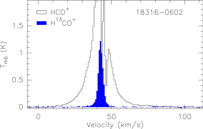
Figure 4: Comparision of the HCO⁺ (1–0) and H¹³CO⁺ (1–0) spectra for 18316$-$0602. No H¹³CO⁺ (1–0) emission is detected at high velocities, which indicates that it is reasonable to assume optically thin emission for the HCO⁺ line wings when deriving the outflow parameters (see Sect. 4.1).

Figure 5: Outflow momentum against $L/M$, for the SiO (2–1) and HCO⁺ (1–0) outflows. Data for SiO (5–4) outflows are indicated as open symbols. Triangles and circles correspond to sources classified as IRL and IRD, respectively (see Table 1). The black dotted line shows the result of a least squares fit to the data, with the Pearson correlation coefficient ($\rho$) shown in the bottom right corner.

Figure 6: Ratio of the outflow mass (derived from the HCO⁺ outflow) to gas mass of the whole molecular clump (derived from N₂H⁺ or C₂H; see Table 8), against $L/M$. Symbols are the same as in Fig. 5. The black dotted lines show the result of least squares fits to the data, with the Pearson correlation coefficient ($\rho$) shown in the bottom right corner.

In Tables 3, 4 and 5, we list the derived outflow parameters for the SiO (2–1), SiO (5–4) and HCO⁺ (1–0) lines, respectively. Assuming an uncertainty of 10% on the flux and 20% on the distance estimates, one finds that this implies uncertainties of 50% for the derived outflow parameters. We have used the SiO abundances derived from the gas mass of the clump (Col. 3 of Table 6). In Tables 3–5, we also list the maximum outflow velocities ($V_{\mathrm{max-b}}$ and $V_{\mathrm{max-r}}$) and the deconvolved lobe sizes (size_blue and size_red). The maximum outflow velocities have been obtained from the difference between the high-velocity limit of the outflow velocity range, $\Delta V$, and the systemic velocity, $V_{\mathrm{LSR}}$. Typical values are in the range 10–20 km s^-1, with some extreme values as for example the $\sim$60 km s^-1 of the red-shifted wing in 18264$-$1152. From the maximum outflow velocities and the lobe sizes we calculated the kinematic timescale as $t_{\mathrm{kin}}=\mathrm{size}/\mathrm{V}_{\mathrm{max}}$. The average of the numbers obtained for the blue and red lobes resulted in the kinematic timescale listed in Tables 3–5, which is typically a few $10^{4}$ yr. Finally, we note that the mass loss rate, mechanical force, and mechanical luminosity can be obtained as $\dot{M}_{\mathrm{out}}=M_{\mathrm{out}}/t_{\mathrm{kin}}$, $F_{\mathrm{out}}=p_{\mathrm{out}}/t_{\mathrm{kin}}$, and $L_{\mathrm{mec}}=E_{\mathrm{out}}/t_{\mathrm{kin}}$, respectively. In the derivation of the outflow parameters we have not corrected for the inclination of the outflow axis with respect to the line of sight. Some outflow parameters, such as the energy and mechanical luminosity, can be greatly affected if inclination $>60\degr$ (see Table 6 of López-Sepulcre et al. 2010, for the correction factor that must be applied for different inclinations).

The median outflow mass loss rate, mechanical force, and mechanical luminosity in our sample are $\sim$$9.1\times 10^{-4}$ $M_{\sun}$ yr^-1, $\sim$$5.8\times 10^{-3}$ $M_{\sun}$ km s^-1 yr^-1, and $\sim$4 $L_{\sun}$, respectively. These values are higher than typical values found in low-mass outflows and similar to those found toward objects with luminosities in the range $10^{3}$–$10^{5}$ $L_{\sun}$ (e. g., Beuther et al., 2002b; Wu et al., 2004; López-Sepulcre et al., 2009), confirming that the molecular outflows reported in this work are associated with high-mass star formation.

Figure 7: SiO abundance determined from the gas mass of the clump (top panel) and from the SiO to HCO⁺ column density ratio (bottom panel) versus $L/M$. Symbols are the same as in Fig. 5. The black dotted lines show the result of least squares fits to the data, with the Pearson correlation coefficient ($\rho$) shown in the bottom left corner.

4.2 Outflow activity with time

Different studies (e. g., Saraceno et al., 1996; Sridharan et al., 2002; Molinari et al., 2008; Giannetti et al., 2013) have proposed the luminosity-to-mass ratio, $L/M$, to be a good measure of the evolutionary phase in the star formation process, with lower values corresponding to less evolved stages. With this in mind, López-Sepulcre et al. (2011) studied the variation of the SiO (2–1) luminosity with $L/M$ for a sample of 47 high-mass YSOs. These authors found a decrease of $L_{\mathrm{SiO}}/L_{\mathrm{bol}}$ with $L/M$ that can be interpreted as either a decrease of the SiO outflow energetics or a decrease of the SiO abundance with time. However, this result was based on single-pointing spectra, and did not make it possible to determine the outflow physical parameters, which are necessary to confirm whether the outflow properties vary with the evolution of the object. Such parameters can be now obtained from the outflow maps presented in this paper (see Sect. 4.1).

In Fig. 5, we plot the outflow momentum with respect to $L/M$, for the SiO and HCO⁺ outflows (similar plots are obtained for the outflow mass and energy). The low number of sources (only fourteen), and the restricted $L/M$ range covered in our observations (<$100$ $L_{\sun}$ $M_{\sun}$^-1), hinder a robust statistical analysis, but it is still possible to search for trends in the plots. No clear variations are found for the SiO outflow momentum as the object evolves (see Fig. 5-top panel), while the HCO⁺ outflow momentum seems to slightly increase with time (with a Pearson correlation coefficient of 0.43, see dotted line in Fig. 5-bottom panel). We note that the trend is majorly dominated by the two sources with the lower $L/M$ values: G19.27$+$0.1M1 and G19.27$+$0.1M2, which could be associated with intermediate-mass rather than high-mass YSOs (see Sect. 3.3). A similar trend is also seen in Fig. 6, where we plot the ratio of the outflow mass (calculated from the HCO⁺ outflow) to the gas mass of the clump, derived from the N₂H⁺ and C₂H emission (see Table 8), which is a distance independent parameter. However, observations of more sources, covering a larger $L/M$ range, are necessary to definitively confirm or rule out a possible increase of the HCO⁺ outflow energetics with time. In Fig. 7-top, we show the SiO abundance as function of $L/M$, while in the bottom panel, we show the same plot using the SiO abundances derived from the SiO to HCO⁺ column density ratio (see Sect. 4.1). In both cases, we find a decrease of the SiO abundance with time (as suggested by Sakai et al. 2010). A least squares fit to the data results in ${\rm X(SiO)_{clump}}=-(0.38\pm 0.07)\,[L/M]-(8.45\pm 0.07)$ and ${\rm X(SiO)_{HCO^{+}}}=-(0.89\pm 0.21)\,[L/M]-(7.67\pm 0.22)$, with correlation coefficients of $-0.5$ and $-0.6$, for the top and bottom panels respectively. These results are consistent with the variation reported by López-Sepulcre et al. (2011) and suggest a scenario in which SiO is largely enhanced in the first evolutionary stages, as expected if SiO is released from dust grains due to strong shocks produced by protostellar jets. As the object evolves, the power of the jet decreases, and so does the intensity of the shocks and the SiO abundance. Throughout this process, however, there is likely an increase of the amount of ambient material that is swept up by the jet, and thus the time-integrated outflow activity, which is traced by entrained molecular material (e. g., HCO⁺), likely increases with the age of the driving source.

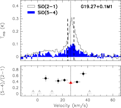
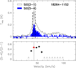
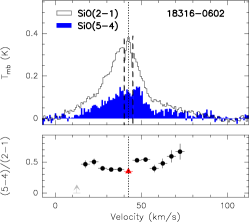
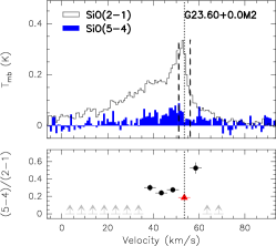
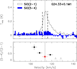
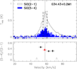
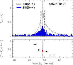
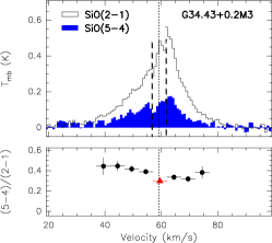
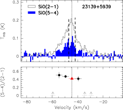
Figure 8: SiO (2–1) and (5–4) spectra obtained from the convolved maps. Each spectrum consists of three different parts: for blue/red-shifted velocities we have extracted the spectrum averaged over the area defined by the 50% contour level of the blue/red-shifted integrated emission (considering the velocity intervals listed in Table 3), and for systemic velocities the area is defined by the 50% contour level of the whole integrated emission. The vertical dashed lines indicate the three distinct velocity regimes, and the dotted vertical line corresponds to the systemic velocity. In the bottom panels (below each spectrum) we plot the (5–4)/(2–1) line ratio for velocity intervals of 5 km s^-1 width. Red triangles correspond to the line ratio at the systemic velocity.

4.3 SiO excitation

We can use the SiO (2–1) and (5–4) maps of the nine sources with clear detections in both lines, to constrain the physical conditions of the outflows and search for differences in the excitation conditions as a function of velocity. To do this, we first convolved the SiO (5–4) and SiO (2–1) maps to the same angular resolution, 30″, and considered two distinct velocity regimes: systemic velocities, corresponding to the range $\pm 2.5$ km s^-1 around the bulk velocity (listed in Table 1), and high velocities, corresponding to the red- and blue-shifted ($|V-V_{\mathrm{LSR}}|>2.5$ km s^-1) outflow velocities.

In Fig. 8, we show the SiO (2–1) and (5–4) spectra for the nine outflow sources. These spectra have been obtained after degrading the resolution of all maps to 30″. In order to take into account that the emission at different velocities comes from different spatial structures: bulk velocity emission and outflow lobes, we extracted the spectra averaged over the area enclosed by the 50% contour level of the corresponding outflow lobe. At systemic velocities, the average was made over the area enclosed by the 50% contour level of the whole integrated emission. The different velocity intervals are indicated in the figure with vertical dashed lines. In the bottom panel associated with each spectrum of Fig. 8, we show the (5–4)/(2–1) line ratio as a function of the velocity, considering velocity intervals of 5 km s^-1. We calculated the line ratio for those velocity intervals in which the line intensity of both transitions is at least 3 times above the noise level, determined by the expression $\sigma=\Delta V\sigma_{\mathrm{rms}}(N)^{1/2}$, with $\Delta V=5$ km s^-1, $\sigma_{\mathrm{rms}}$ the rms of the spectrum, and $N$ the number of channels (e. g., Caselli et al., 2002a). We find that for most of the sources, the (5–4)/(2–1) line ratio is typically low at the systemic velocity and increases as we move to red/blue-shifted velocities. This effect is clear in Fig. 9, in which the x-axis shows the (5–4)/(2–1) line ratio normalized with respect to the line ratio measured at systemic velocities. This normalization permits us to remove calibration errors. For increasing velocities (with respect to the systemic) we find a ratio slightly greater than unity (see star symbols in Fig. 9). The distribution of the normalized line ratios for red/blue-shifted velocities (see top panel of Fig. 9) has an average value of 1.39. This result indicates that the excitation conditions for SiO depend on the velocity of the emitting gas. The same trend has been found in some well-studied low-mass protostellar outflows (e. g., L1157 and L1448: Nisini et al. 2007).

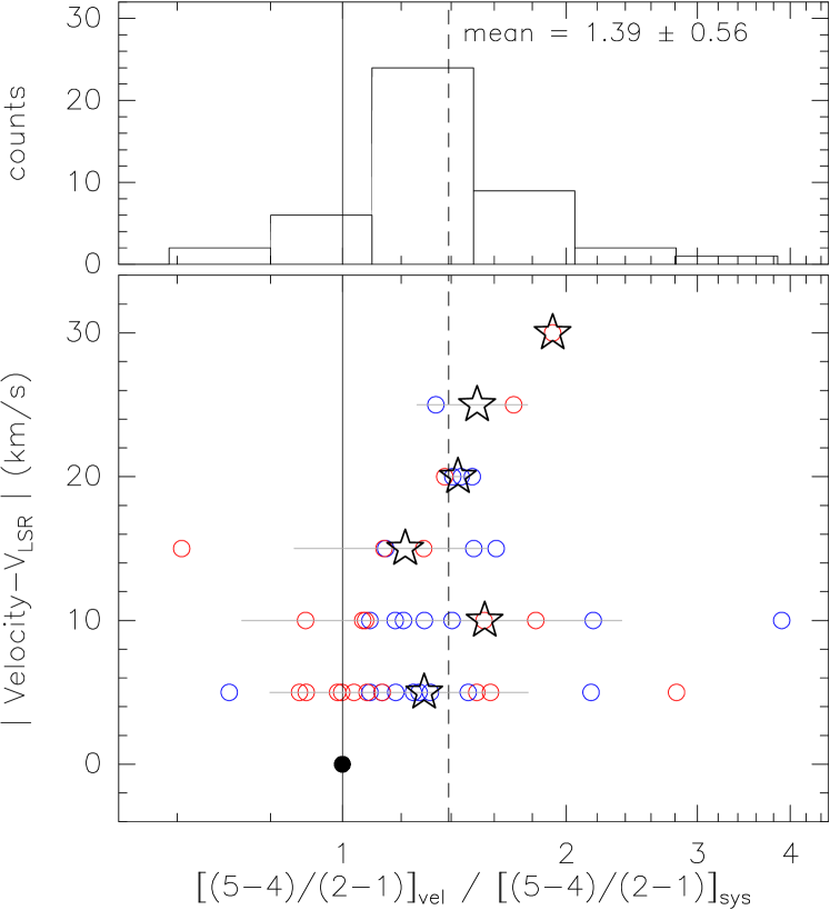
Figure 9: Bottom panel: Velocity, with respect to the systemic velocity, against the SiO (5–4)/(2–1) line ratio, normalized with the line ratio measured at systemic velocities. The black dot corresponds to the normalized line ratio equal to unity that corresponds to the systemic velocity. Red and blue circles correspond to the red and blue-shifted SiO emission. Stars (and horizontal gray lines) indicate the mean (and dispersion) value at each velocity. The vertical dashed line indicates the mean value for all the line ratios at velocities higher than the systemic velocity. Top panel: Distribution of normalized SiO (5–4)/(2–1) line ratios. The mean (and dispersion) value, corresponding to 1.39 (0.56) is indicated with the vertical dashed line.

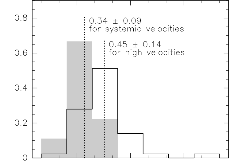
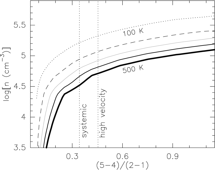
Figure 10: Top panel: Distributions of the SiO (5–4)/(2–1) ratio for two different velocity regimes: systemic velocities (gray filled histogram) and high velocities (solid line histogram). The dotted line and numbers indicate the mean ($\pm$standard deviation) value. Bottom panel: LVG results produced by the RADEX code. We plot the density versus the SiO (5–4)/(2–1) ratio. The curves correspond to kinetic temperatures ranging from 100 K (upper curve) to 500 K (lower curve) in steps of 100 K. The two vertical lines correspond to the mean (5–4)/(2–1) ratios for systemic and high velocities.

4.3.1 Collisional excitation calculations

The results derived from Figs. 8 and 9, indicate that the excitation conditions differ between the gas components at systemic and high velocities. To constrain the corresponding physical conditions, we performed radiative transfer calculations with the RADEX code (van der Tak et al., 2007) based on the large velocity gradient (LVG) approximation and assuming a plane-parallel “slab” geometry. The molecular data were retrieved from the LAMDA data base. The collisional rate coefficients were calculated between SiO and H₂, incorporating levels up to $J=40$ for kinetic temperatures up to 2000 K (Dayou & Balança, 2006). In Fig. 10-top, we show the distribution of the (5–4)/(2–1) ratio values obtained for the two different velocity regimes: systemic velocities (gray filled histogram) and high velocities (solid line histogram). The mean (and standard deviation) values of the line ratios are $0.34\pm 0.09$ and $0.45\pm 0.14$ for systemic and high velocities, respectively. In Fig. 10-bottom, we compare these mean line ratios with the results obtained from the RADEX analysis. RADEX calculations were obtained with a velocity dispersion of 5 km s^-1, and a column density of $10^{12}$ cm^-1, i. e., optically thin emission (the modeled line ratios are insensitive to the column density up to values of $10^{13}$ cm^-2). The different curves shown in the figure correspond to kinetic temperatures ranging from 100 K to 500 K, which is a range of temperatures typically found toward low- and high-mass outflows (e. g., Nisini et al., 2007; Codella et al., 2013). From this analysis we can infer that in general the SiO emission of our outflow sources is generated from shocks in regions with densities ranging from $10^{4.0}$ cm^-3 to $10^{5.5}$ cm^-3, for kinetic temperatures in the range 100–500 K. From the mean values of the SiO (5–4)/(2–1) ratio (see Fig. 10-bottom), the range of densities is $10^{4.7}$–$10^{5.3}$ cm^-3 for high velocities, and $10^{4.4}$–$10^{5.2}$ cm^-3 for low velocities, which are hints of the gas at high velocities to be produced in regions with larger densities (and/or temperatures) than the gas at systemic velocities.

4.4 SiO production

SiO is known to have an extremely low abundance in dark clouds (e. g., Ziurys et al., 1989) or in photon-dominated regions (PDRs; e. g., Schilke et al. 2001) whereas it is easily detected in outflows. Partly as a consequence, most theoretical work on the SiO abundance in star-forming regions has centered on the abundance in outflows and jets where it seems likely that shock chemistry plays a major role (e. g., Schilke et al., 1997; Gusdorf et al., 2008a, b, 2011). Three general scenarios have been discussed: (1) Si production due to sputtering of grain cores followed by gas phase reactions with O₂ or OH, (2) sputtering of SiO mixed into grain mantles, and (3) grain-grain collisions liberating Si from cores. The first and third of these require relatively high shock velocities in order to produce an observable quantity of SiO (at least 25 km s^-1 in the case of option 1, though perhaps less in the case of grain-grain collisions). Such high shock velocities seem unlikely for our observed outflows which in general (see $\Delta V_{\mathrm{red}}$ and $\Delta V_{\mathrm{blue}}$ in Tables 3 and 4) show SiO emission at velocities (relative to ambient) less than 30 km s^-1 with notable exceptions such as 18316$-$0602 and G23.60$+$0.0M2. Also we note that our observed profiles (see Figs. 1 and 8) show mainly emission at velocities only a few km s^-1 different from the systemic velocity with a high velocity tail suggesting again that low 10–15 km s^-1 shocks predominate, similar to what is found in the low-mass protostellar outflow L1157 (Nisini et al., 2007). In this sense, it is interesting to note that Gusdorf et al. (2008b) conclude that SiO mixed into grain mantles is necessary to explain the observations towards the shock region L1157 B1. This seems plausible also in the regions we have studied though we note that the absence of detections of a solid state SiO feature gives pause for thought. Moreover, the very low SiO abundances found by Schilke et al. (2001) towards nearby PDRs are slightly surprising if several percent of silicon are in the form of mantle material. However, present estimates of photodesorption yields from ice mantles are extremely crude and we conclude that the most likely scenario explaining our results is a gradual erosion of ice mantles as the clump evolves resulting in less SiO being ejected into the outflow shocked material at late times.

5 Summary

We have mapped 14 high-mass star-forming regions with the IRAM 30-m telescope in different molecular lines at 1 and 3 mm, with the aim to characterize the properties of molecular outflows associated with high-mass YSOs. The sample was selected from the work of López-Sepulcre et al. (2011), and contains objects with previous single-pointing SiO molecular outflow emission. Our main conclusions can be summarized as follows:

• The wide ($\sim$15 GHz) frequency range surveyed has allowed us to simultaneously map several molecular transitions, typically found tracing dense gas (e. g., N₂H⁺, C₂H, NH₂D) and outflow (e. g., SiO, HCO⁺) emission. Twelve of the fourteen sources, are also detected in the CH₃CN line (eight of them showing emission of high excitation $K$ transitions), which is a tracer typically found in association with hot cores.

• The detection of high-velocity wings in the SiO (2–1) and HCO⁺ (1–0) lines for all the sources, confirms the presence of outflows in these regions as previously reported by López-Sepulcre et al. (2010, 2011). The outflow maps reveal clear bipolar structures in six of the regions.

• We improved the SEDs of these sources by complementing previous continuum data with Hi-GAL data (Molinari et al., 2010a, b). From the SEDs we derived dust envelope masses and luminosities in the range 100-3000 $M_{\sun}$ and 100–50000 $L_{\sun}$, respectively. We calculated the luminosity-to-mass ratio, $L/M$, which is believed a good indicator of the evolutionary stage.

• We studied the variation of the outflow properties as the object evolves. The SiO outflow energetics seem to remain constant with time (i. e., $L/M$), while there are some hints of a possible trend suggesting that the HCO⁺ outflow energetics might increase as the object evolves. Interestingly, we find a decrease of the SiO abundance with time, from $10^{-8}$ to $10^{-9}$. There results are consistent with the variation reported by López-Sepulcre et al. (2011), and suggest a scenario in which SiO is largely enhanced in the first evolutionary stages, probably due to strong shocks originated by the protostellar jet. As the object evolves, the power of the jet would decrease and so would the SiO abundance. In the meanwhile, the material surrounding the protostar would have been swept up by the jet, and thus the outflow activity, as traced by entrained molecular material (HCO⁺), would increase with time.

• We find that the SiO (5–4)/(2–1) line ratio is typically low at systemic velocities, and increases as we move to red/blue-shifted velocities, as similarly found toward low-mass protostellar outflows (e. g., Nisini et al., 2007). From radiative transfer calculations done with the RADEX code, we find that, in general, the SiO emission of our outflows is generated in regions with densities $10^{4.0}$–$10^{5.5}$ cm^-3 and kinetic temperatures 100–500 K, with larger densities and/or temperatures for the high-velocity gas component.

Appendix A Figures, molecular line results and spectral energy distributions

Table 7: Molecular lines detected at 3 mm toward the 14 high-mass young stellar objects^a

Molecular	Freq.
transition	(MHz)	#01	#02	#03	#04	#05	#06	#07	#08	#09	#10	#11	#12	#13	#14
NH2D (11,1–10,1)b	85926.2780	Y	Y	Y	Y	Y	n	Y	Y	Y	Y	Y	Y	n	n
HC15N (1–0)	86054.9664	Y	n	n	Y	Y	n	Y	Y	Y	Y	n	Y	n	n
SO (22–11)	86093.9500	Y	n	Y	Y	Y	n	Y	Y	n	Y	n	Y	Y	Y
H13CN (12–01)b	86340.1630	Y	Y	Y	Y	Y	Y	Y	Y	Y	Y	Y	Y	Y	Y
HCO (10,1–00,0)b	86670.7600	Y	n	Y	n	Y	n	n	n	n	n	n	n	n	Y
H13CO+ (1–0)	86754.2884	Y	Y	Y	Y	Y	Y	Y	Y	Y	Y	Y	Y	Y	Y
SiO (2–1)	86846.9600	Y	Y	Y	Y	Y	Y	Y	Y	Y	Y	Y	Y	Y	Y
HN13C (1–0)	87090.8252	Y	Y	Y	Y	Y	Y	Y	Y	Y	Y	Y	Y	Y	Y
C2H (1–0)b	87316.8980	Y	Y	Y	Y	Y	Y	Y	Y	Y	Y	Y	Y	Y	Y
HC5N (33–32)	87863.6300	Y	n	n	n	n	n	n	n	Y	n	n	n	n	n
HNCO (40,4–30,3)	87925.2370	Y	Y	Y	Y	Y	Y	Y	Y	Y	Y	Y	Y	n	Y
HCN (12–00)b	88631.8475	Y	Y	Y	Y	Y	Y	Y	Y	Y	Y	Y	Y	Y	Y
H15NC (1–0)	88865.7150	Y	n	Y	n	Y	n	Y	Y	Y	n	n	Y	n	n
HCO+ (1–0)	89188.5247	Y	Y	Y	Y	Y	Y	Y	Y	Y	Y	Y	Y	Y	Y
HNC (1–0)	90663.5680	Y	Y	Y	Y	Y	Y	Y	Y	Y	Y	Y	Y	Y	Y
HC3N (10–9)	90979.0230	Y	Y	Y	Y	Y	Y	Y	Y	Y	Y	Y	Y	Y	Y
CH3CN (50–40)c	91987.0876	Y	Y	Y	Y	Y	n	Y	Y	Y	Y	Y	Y	Y	n
13CS (2–1)	92494.3080	Y	Y	Y	Y	Y	n	Y	Y	Y	Y	Y	Y	Y	Y
N2H+ (12,3–01,2)b	93173.7642	Y	Y	Y	Y	Y	Y	Y	Y	Y	Y	Y	Y	Y	Y

• Y: line detected. n: line non detected. The frequencies are obtained from the CDMS (Cologne Database for Molecular Spectroscopy; Müller et al. 2001) and JPL (Jet Propulsion Laboratory; Pickett et al. 1998) catalogues.

• Transition and frequency of the main hyperfine component. For a few species, the different hyperfine components are well separated in frequency: for HCO, we detect four hyperfine components at 86670.76 MHz, 86708.36 MHz, 86777.46 MHz and 86777.46 MHz; and for C₂H, we detect six hyperfine components at 87284.105 MHz, 87316.898 MHz, 87328.585 MHz, 87401.989 MHz, 87407.165 MHz and 87446.470 MHz.

• For some sources we detect several transits of the $k$-ladder spectrum of the CH₃CN (5–4) transition, corresponding to the frequencies 91987.0876 MHz ($K=0$), 91985.3141 MHz ($K=1$), 91979.9943 MHz ($K=2$), 91971.1304 MHz ($K=3$), and 91958.7260 MHz ($K=4$).

In Figure 11, we present different panels for each observed source, including the spectra at 3 mm, zero-order moment (integrated intensity) maps for different molecular lines, and a comparison between the emission at 8 $\mu$m and at sub-millimeter (500 $\mu$m or 850 $\mu$m) wavelengths. In Table 7, we list the detection of molecules toward the 14 high-mass YSOs, while in Table 8, we list the hyperfine structure fit results and physical parameters of the dense cores derived from the N₂H⁺ (1–0) and C₂H (1–0) lines. In Table 9, we present continuum fluxes measured for the 14 sources, in the wavelength range from 8.0 $\mu$m to 1.2 mm, including data from different facilities: MSX, Spitzer/MIPS, IRAS, Herschel/PACS, Herschel/SPIRE, JCMT, APEX and IRAM 30m. Finally, in Fig. 12 we show the SEDs for the 14 objects, with the observational parameters listed in Table 9 and the best fit as explained in Sect. 3.3.

Table 8: Hyperfine structure fit results and physical parameters of dense cores derived from N₂H⁺ (1–0) and C₂H (1–0) lines

		$V_{\mathrm{LSR}}$b	$\Delta V$b		$T_{\mathrm{ex}}$c	$N_{\mathrm{mol}}$c	size	$M_{\mathrm{gas}}$d
ID	$A\times\tau$a	(km s-1)	(km s-1)	$\tau$a	(K)	(cm-2)	(″)	($M_{\sun}$)
N2H+ (1–0)
01	$1.28\pm 0.01$	0$+33.01\pm 0.01$	$2.12\pm 0.01$	$0.17\pm 0.01$	10.68	0$3.25\times 10^{12}$	38	0320
02	$1.21\pm 0.02$	0$+26.88\pm 0.01$	$2.64\pm 0.02$	$0.31\pm 0.02$	06.94	0$3.45\times 10^{12}$	40	0250
03	$1.72\pm 0.01$	0$+26.56\pm 0.01$	$2.79\pm 0.01$	$0.29\pm 0.01$	09.13	0$5.42\times 10^{12}$	33	0270
04	$1.83\pm 0.03$	0$+26.50\pm 0.01$	$2.54\pm 0.02$	$0.19\pm 0.02$	13.00	0$6.08\times 10^{12}$	42	0520
05	$2.00\pm 0.01$	0$+43.56\pm 0.01$	$2.80\pm 0.01$	$0.10\pm 0.01$	23.19	$10.70\times 10^{12}$	31	0990
06	$1.35\pm 0.05$	$+106.58\pm 0.02$	$3.54\pm 0.04$	$0.31\pm 0.04$	07.43	0$5.20\times 10^{12}$	21	2010
07	$1.88\pm 0.01$	0$+42.60\pm 0.01$	$3.28\pm 0.01$	$0.23\pm 0.01$	11.45	0$7.59\times 10^{12}$	58	0670
08	$1.13\pm 0.01$	0$+53.48\pm 0.01$	$2.94\pm 0.03$	$0.29\pm 0.01$	06.99	0$3.60\times 10^{12}$	45	0870
09	$2.44\pm 0.02$	$+113.64\pm 0.01$	$3.33\pm 0.01$	$0.64\pm 0.01$	06.83	0$8.80\times 10^{12}$	39	4810
10	$3.89\pm 0.01$	0$+57.85\pm 0.01$	$3.03\pm 0.01$	$0.12\pm 0.01$	36.28	$32.22\times 10^{12}$	40	5460
11	$3.45\pm 0.02$	0$+57.50\pm 0.01$	$3.36\pm 0.01$	$0.18\pm 0.01$	22.50	$21.68\times 10^{12}$	43	4330
12	$1.72\pm 0.01$	0$+59.20\pm 0.01$	$2.71\pm 0.01$	$0.10\pm 0.01$	20.39	0$8.10\times 10^{12}$	44	1700
13	$0.30\pm 0.01$	0$+43.94\pm 0.05$	$4.64\pm 0.09$	$0.10\pm 0.03$	05.98	0$1.52\times 10^{12}$	29	0110
14	$0.54\pm 0.01$	0$-44.51\pm 0.01$	$2.36\pm 0.01$	$0.10\pm 0.01$	08.48	0$1.41\times 10^{12}$	24	0150
C2H (1–0)
01	$1.62\pm 0.01$	0$+32.97\pm 0.80$	$2.69\pm 2.66$	$0.10\pm 0.10$	19.37	$17.20\times 10^{13}$	58	3650
02	$0.39\pm 0.05$	0$+26.79\pm 0.04$	$2.56\pm 0.14$	$0.46\pm 0.30$	03.68	0$4.09\times 10^{13}$	43	0290
03	$0.55\pm 0.03$	0$+26.35\pm 0.02$	$2.97\pm 0.07$	$1.05\pm 0.15$	03.32	0$9.31\times 10^{13}$	41	0630
04	$1.21\pm 0.10$	0$+26.55\pm 0.04$	$3.14\pm 0.10$	$2.23\pm 0.30$	03.34	$21.10\times 10^{13}$	55	2790
05	$1.12\pm 0.01$	0$+43.83\pm 0.01$	$3.10\pm 0.01$	$0.10\pm 0.01$	14.30	$11.30\times 10^{13}$	37	1320
06	$0.60\pm 0.07$	$+106.35\pm 0.06$	$3.85\pm 0.18$	$0.14\pm 0.38$	07.34	0$5.83\times 10^{13}$	48	3620
07	$0.81\pm 0.01$	0$+42.41\pm 0.01$	$4.35\pm 0.02$	$0.10\pm 0.01$	11.24	$10.10\times 10^{13}$	51	1740
08	$0.57\pm 0.07$	0$+53.57\pm 0.04$	$2.68\pm 0.15$	$0.61\pm 0.31$	03.78	0$5.94\times 10^{13}$	44	1210
09	$0.51\pm 0.01$	$+113.51\pm 0.01$	$3.69\pm 0.06$	$0.10\pm 0.01$	08.03	0$4.77\times 10^{13}$	35	1770
10	$1.25\pm 0.05$	0$+58.00\pm 0.02$	$3.34\pm 0.06$	$0.72\pm 0.11$	04.65	$12.10\times 10^{13}$	30	1040
11	$1.49\pm 0.03$	0$+57.62\pm 0.01$	$4.04\pm 0.04$	$1.36\pm 0.07$	03.95	$21.40\times 10^{13}$	42	3620
12	$0.71\pm 0.03$	0$+59.23\pm 0.02$	$3.02\pm 0.06$	$0.32\pm 0.10$	05.17	0$5.75\times 10^{13}$	43	1000
13	$0.64\pm 0.02$	0$+43.87\pm 0.05$	$5.58\pm 0.12$	$0.10\pm 0.02$	09.42	0$9.45\times 10^{13}$	31	0660
14	$0.76\pm 0.01$	0$-44.45\pm 0.01$	$2.96\pm 0.03$	$0.10\pm 0.02$	10.65	0$6.25\times 10^{13}$	32	1010

• Parameters obtained from the CLASS fit with $A=f[J_{\nu}(T_{\mathrm{ex}})-J_{\nu}(T_{\mathrm{bg}})]$, and $\tau$ the optical depth of the main hyperfine, adopted to be the ($1_{2,3}$–$0_{1,2}$) line for the N₂H⁺ and the ($1_{2,2}$–$0_{1,1}$) line for the C₂H.

• Systemic velocity, $V_{\mathrm{lsr}}$, and linewidth, $\Delta V$, both in km s^-1.

• Excitation temperature, $T_{\mathrm{ex}}$, in K, and molecular column density, $N_{\mathrm{mol}}$, in cm^-2.

• Mass of the gas calculated as $M_{\mathrm{gas}}=(N_{\mathrm{mol}}/X)\,\mu\,m_{\mathrm{H}}$ Area, where Area$=\pi\,\mathrm{size}/2$, $m_{\mathrm{H}}$ is the mass of the hydrogen atom, $\mu$ is the molecular weight ($=16$ for N₂H⁺ and $=14$ for C₂H), and $X$ is the abundance with respect to H₂ (fixed to $3\times 10^{-10}$ for N₂H⁺ and $3\times 10^{-9}$ for C₂H; e. g., Huggins et al. 1984; Caselli et al. 2002b; Beuther et al. 2008; Padovani et al. 2009; Busquet et al. 2011; Frau et al. 2012).

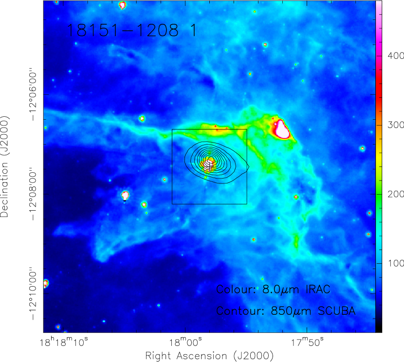
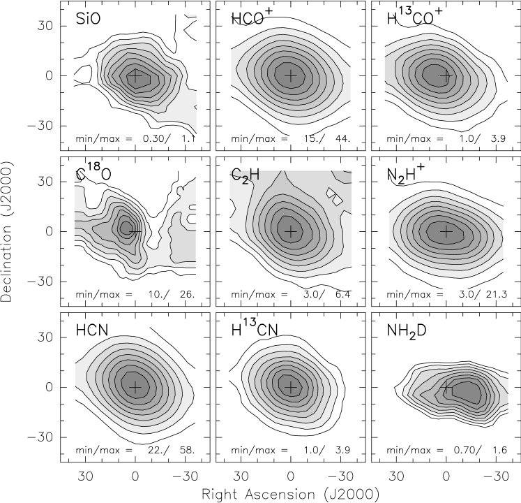
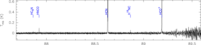
Figure 11: Top-left: Hi-GAL 500 $\mu$m (or JCMT 850 $\mu$m) continuum image in contours overlaid on the Spitzer/IRAC 8.0 $\mu$ (or MSX 8.3 $\mu$m) image in color scale. The box show the region mapped with the IRAM 30-m telescope. Top-right: nine panels with the zero-order moment (velocity-integrated intensity) maps of different molecular species (labeled in the top-left corner of each panel). The minimum and maximum contour level (in units K km s^-1) is indicated in the bottom part of each panel. Bottom: four panels with the IRAM 30-m spectra at 3 mm, covering a frequency range from 87.6 GHz to 93.4 GHz.

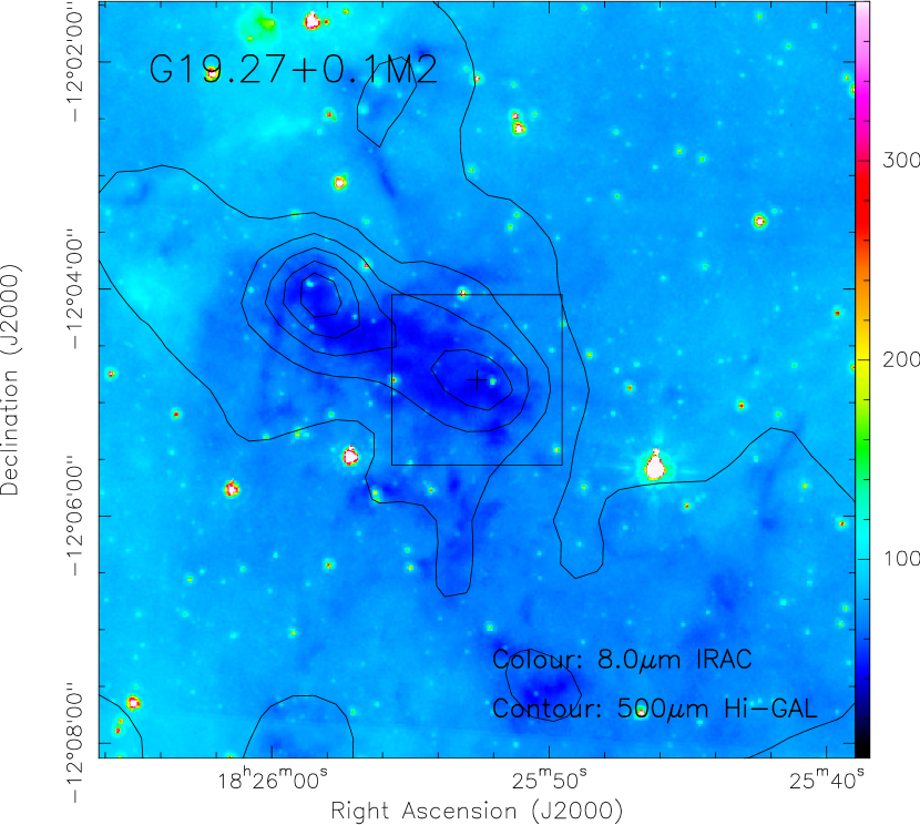
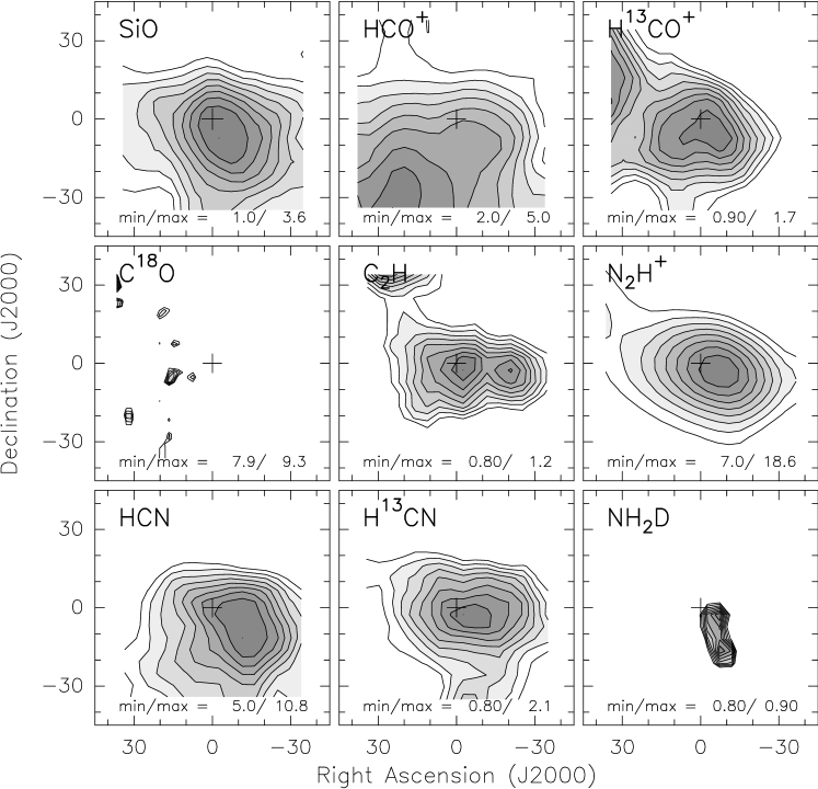
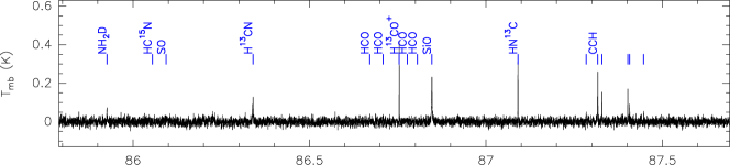
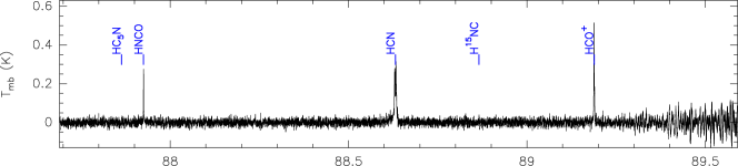
Figure 11: continued, for G19.27$+$0.1 M2.

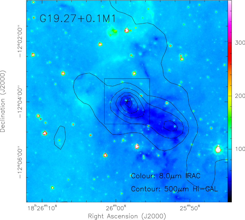
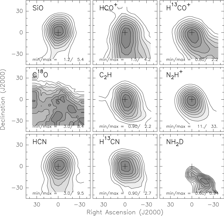
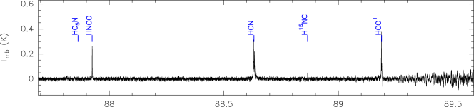
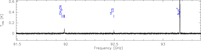
Figure 11: continued, for G19.27$+$0.1 M1.

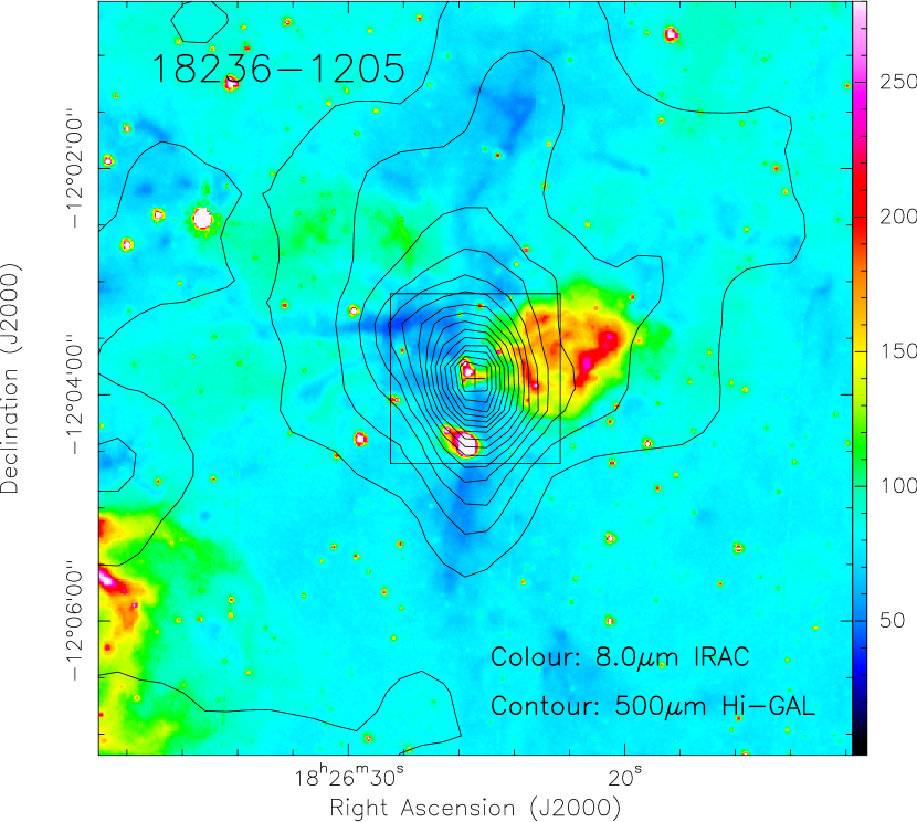
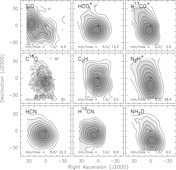
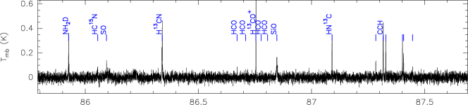
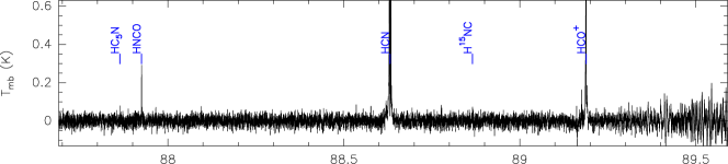
Figure 11: continued, for 18236$-$1205.

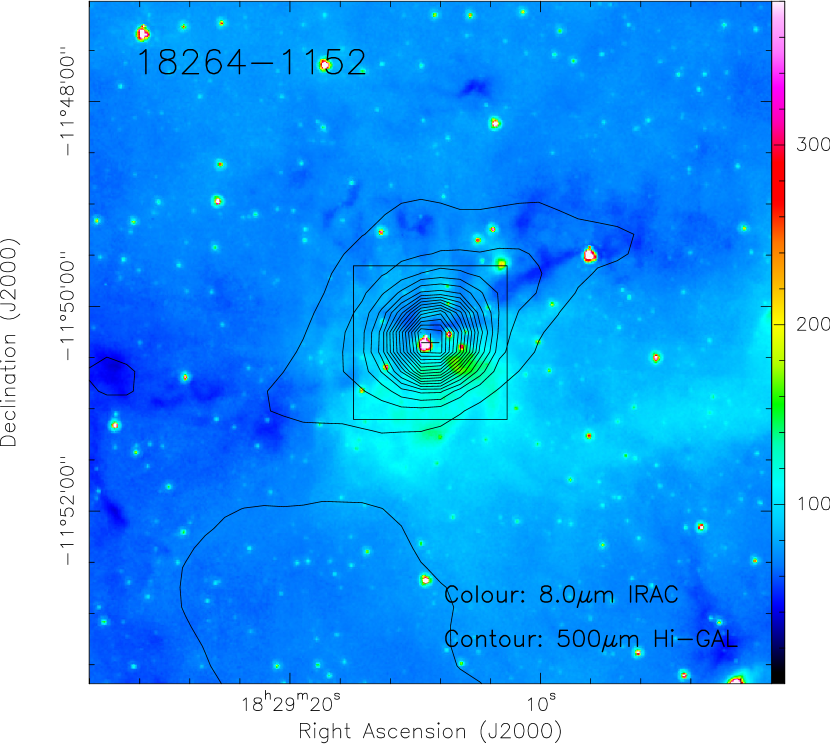
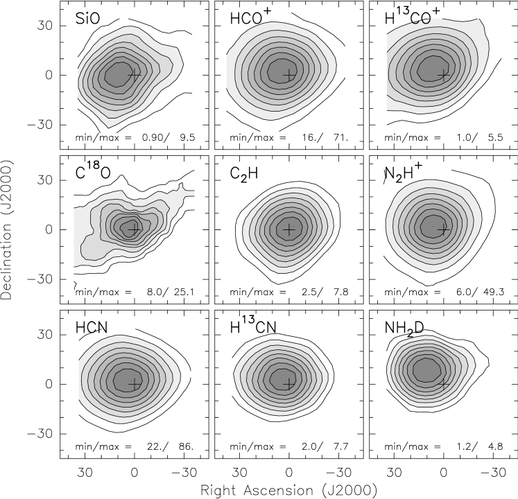
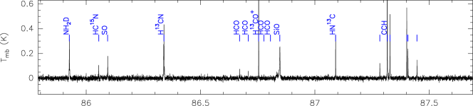
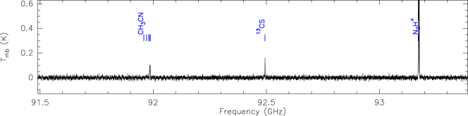
Figure 11: continued, for 18264$-$1152.

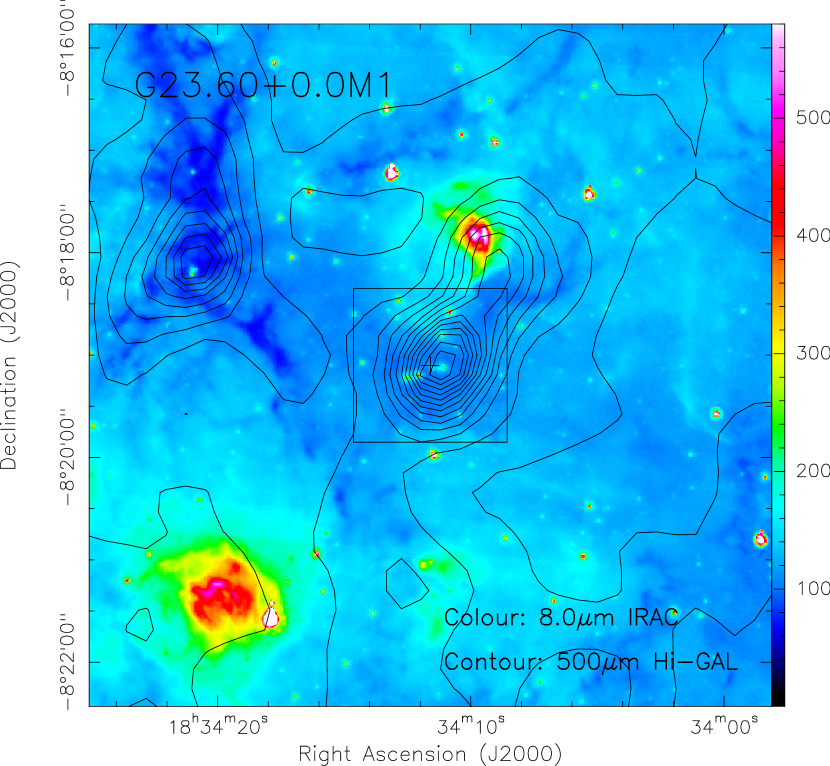
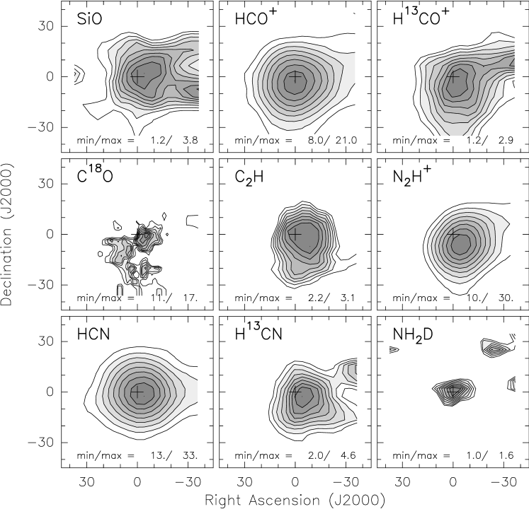
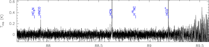
Figure 11: continued, for G23.60$+$0.0 M1.

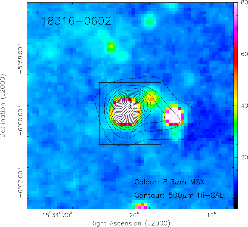
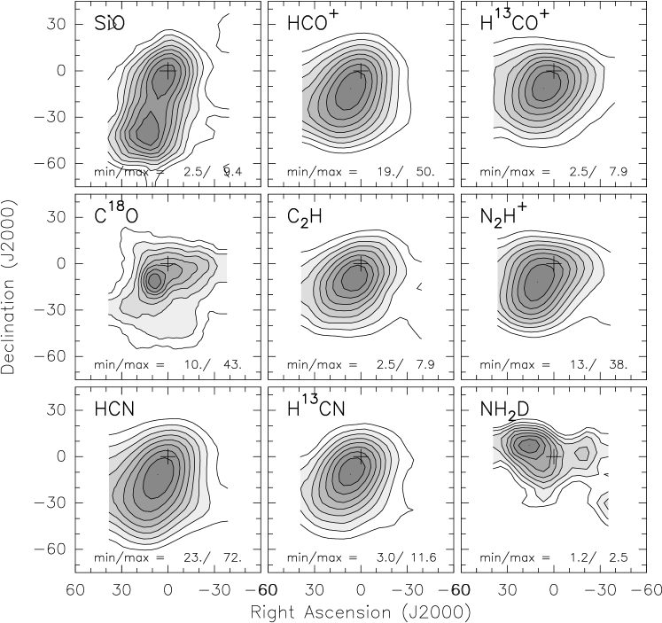
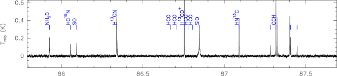
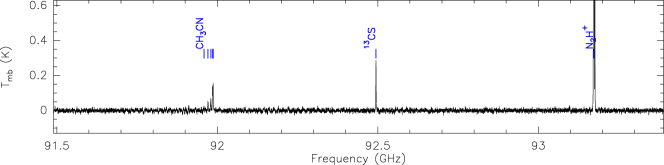
Figure 11: continued, for 18316$-$0602.

Table 9: Measured continuum fluxes, in Jy, from mid-IR to millimeter wavelengths

		Spectral Energy Distributions for our sources
		#01	#02	#03	#04	#05	#06	#07	#08	#09	#10	#11	#12	#13	#14
MSXa	8.3 $\mu$m	10.3	$<$0.2	$<$0.2	0.2	0.6	$<$0.2	19.5	$<$0.2	$<$0.2	$<$0.1	1.2	$<$0.2	2.0	2.1
IRASb	12 $\mu$m	19.0	—	—	2.9	2.9	—	22.8	—	$<$5	$<$1.4	$<$1.4	—	5.3	2.9
MSXa	12.1 $\mu$m	21.8	$<$0.6	$<$0.6	$<$0.5	$<$0.5	$<$0.6	15.6	$<$0.6	$<$0.6	$<$0.8	1.8	$<$0.6	3.1	3.0
MSXa	14.7 $\mu$m	33.0	$<$0.6	$<$0.6	0.9	0.7	$<$0.6	26.3	$<$0.6	$<$0.6	$<$0.6	2.2	$<$0.6	6.1	5.4
MSXa	21.3 $\mu$m	61.8	$<$1.1	$<$1.1	5.5	3.4	$<$1.1	69.7	$<$1.1	$<$1.1	4.1	13.6	$<$1.1	46.7	24.3
MIPSc	24 $\mu$m	—	0.02	0.24	$>$6	5.4	0.22	—	1.8	4.4	$>$6	$>$10	0.25	$>$18	—
IRASb	25 $\mu$m	98.6	—	—	14.3	11.1	—	137.6	—	5.9	$<$27.2	$<$27.2	—	129.1	50.1
IRASb	60 $\mu$m	891	—	—	324	317	—	958	—	187	$<$765	$<$765	—	1725	367
MIPSc	70 $\mu$m	—	—	—	260	291	15	—	44	245	479	321	14	—	—
HiGALd	70 $\mu$m	—	—	14.3	280.8	386.3	33.7	1200	98.4	659.8	942.0	338.4	38.7	2212	—
IRASb	100 $\mu$m	1891	—	—	1028	1104	—	2136	—	727	$<$1948	$<$1948	—	2744	$<$686
HiGALd	160 $\mu$m	—	—	55.6	400.2	725.5	139.5	1590	169.2	866.0	1120	587.0	91.7	1598	—
HiGALd	250 $\mu$m	—	—	63.8	328.8	464.5	165.0	623	117.6	496.3	585.5	538.6	97.0	682.2	—
HiGALd	350 $\mu$m	—	—	29.3	130.4	229.2	81.7	359	44.2	229.1	326.3	270.1	52.1	385.8	—
JCMTe	450 $\mu$m	83	14	25	194	—	—	—	—	—	148	—	38	$<$351	76
HiGALd	500 $\mu$m	—	23.3	13.1	47.3	66.4	32.8	116	13.6	73.7	82.3	95.5	20.5	84.9	—
JCMTe	850 $\mu$m	9.53	2.88	3.83	20.4	13.4	—	—	—	—	16.7	—	5.26	16.7	6.32
APEXf	850 $\mu$m	—	3.13	3.43	16.8	20.6	5.95	25.6	3.29	9.75	—	—	—	—	—
—g	1.2 mm	3.60	0.92	0.91	10.4	7.6	1.11	10.6	0.71	2.03	4.01	13.2	1.02	5.3	2.30

• Fluxes obtained from the catalog of the Midcourse Space Experiment (MSX; Price et al. 1999).

• Fluxes obtained from the point source catalog v2.1 of the Infrared Astronomical Satellite (IRAS; Neugebauer et al. 1984).

• Fluxes obtained from the Spitzer satellite, and the instrument Multiband Imaging Photometer for Spitzer (MIPS; Rieke et al. 2004).

• Fluxes obtained from the Hi-GAL/Herschel project (Molinari et al. 2010a, b).

• Fluxes obtained from the SCUBA Legacy survey (Di Francesco et al. 2008).

• Fluxes obtained from the ATLASGAL project (Schuller et al. 2009).

• At 1.2 mm we used the single-dish surveys of Beuther et al. (2002a); Faúndez et al. (2004); Hill et al. (2005); Rathborne et al. (2006), carried out with the IRAM 30 m telescope or with the SEST (Swedish-ESO 15m Submillimeter Telescope).