Abstract

In this paper we give a bijective proof for a relation between uni- bi- and tricellular maps of certain topological genus. While this relation can formally be obtained using Matrix-theory as a result of the Schwinger-Dyson equation, we here present a bijection for the corresponding coefficient equation. Our construction is facilitated by repeated application of a certain cutting, the contraction of edges, incident to two vertices and the deletion of certain edges.

1 Introduction

$k$-cellular maps can be viewed as drawings on a topological surface, they represent a cell-complex of the latter and inherit the topological genus of the surface as their geometric realization.

In a seminal paper Harer and Zagier [13] computed the virtual Euler characteristic of the Moduli space of curves, independently derived by Penner [9] and still lack a combinatorial interpretation. Key object here play unicellular maps [4] of genus $g$ with $n$ edges, $U_{g}(n)$, i.e. fatgraphs[10, 8, 7] with a unique boundary component. Most prominantly here is the recursion

$$(n+1){\sf u}_{g}(n)=2(2n-1){\sf u}_{g}(n-1)+(2n-1)(n-1)(2n-3){\sf u}_{g-1}(n-2)$$

In [14, 2] the generating function of unicellular maps is obtained as

$${\bf U}_{g}(z)=\frac{P_{g}(z)}{(1-4z)^{3g-1/2}},$$

where $P_{g}(z)$ is polynomial defined over the integers of degree at most $3g-1$ that is divisible by $z^{2g}$ with $P_{g}(1/4)\neq 0$, $[z^{2g}]P_{g}(z)\neq 0$ and $[z^{h}]P_{g}(z)=0$ for $0\leq h\leq 2g-1$.

Matrix-theory [3, 12], via the Schwinger-Dyson equation or representation theorey [11], connects the generating functions of unicellular, ${\bf U}_{g}(z)$, and bicellular maps, ${\bf B}_{g}(z)$. The latter counts fatgraphs having two boundary components that are connected as combinatorial graphs. The relation can also be proved using the representation theoretic framework of Zagier [14] and is given by

$$\sum_{g_{1}=0}^{g+1}\,{\bf U}_{g_{1}}(z){\bf U}_{g+1-g_{1}}(z)+{\bf B}_{g}(z)={\bf U}_{g+1}(z)/z.$$ (1.1)

Recently [5] the authors presented a bijective proof of the corresponding coefficient equation

$$\sum_{g_{1}=0}^{g+1}\,\sum_{i\geq 0}^{n}\,{\sf u}_{g_{1}}(i){\sf u}_{g+1-g_{1}}(n-i)+{\sf b}_{g}(n)={\sf u}_{g+1}(n+1),$$ (1.2)

which revealed a simple construction mechanism. The bijective proof can for instance be applied, to significantly speed up the folding of RNA interaction structures [6, 1].

An analogous relation between unicellular, bicellular and tricellular maps can also be obtained via Matrix-theory. In this paper we give a bijective proof of this relation which reads

$$\begin{split}&{\sf u}_{g+2}(n+2)=\\ &{\sf t}_{g}(n)+{\sf d}_{g+2}(n)+4{\sf u}_{g+2}(n+1)-3{\sf u}_{g+2}(n)+(n+1)(2n+1){\sf u}_{g+1}(n),\end{split}$$ (1.3)

where ${\sf d}_{g+2}(n)$ is explicitly expressed via numbers of unicellular and bicellular maps.

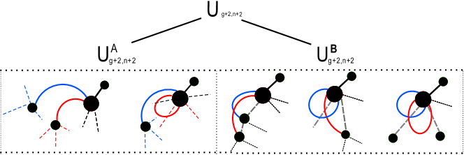
Our strategy is to derive a partition of the set of unicellular maps of genus $(g+2)$ with $(n+2)$ edges, see Fig. 1 for a first step of how to decompose the latter.

Fig. 1: The first step of partition of $U_{g+2,n+2}$.

It is interesting to note that Matrix-theory does not provide any insight w.r.t. for instance quadricellular maps. It seems in fact unlikely that such relations can be derived using this formal framework. The bijective proof presented here however is rather straightforward once the correct partitioning is identified. We believe that it is very well possible to prove similar relations for cellular maps with more than three boundary components.

2 Basic Definitions

Let $S_{2n}$ denote the permutation group over $2n$ elements.

Definition 1.

Let $k,J$ be positive integers. A $k$-cellular map is a triple $(H,\alpha,(\gamma_{i})_{1\leq i\leq k})$, where $H$ is a set of cardinality $2n$, $\alpha$ a fixed-point free involution and $\gamma_{i}$ are cycles such that $\gamma=\prod^{k}_{i=1}\gamma_{i}\in S_{2n}$. The elements of $H$ are half-edges, the cycles of $\alpha$ are edges. The cycles of the permutation $\sigma=\alpha\circ\gamma$ are the vertices $v_{i}$, $1\leq i\leq J$. The length of $v_{i}$ is its degree. The cycle $\gamma_{i}$ is the $i$-th face.

The combinatorial graph $G$ of a $k$-cellular map is the graph whose edges and vertices are the cycles of $\alpha$ and $\sigma$. We can regard a $G$-edge as a ribbon whose two sides are labeled by the half-edges as follows: each side of the ribbon represents one half-edge, we decide which half-edge corresponds to which side of the ribbon by the convention that, if a half-edge $h$ belongs to a cycle $e$ of $\alpha$ and a certain $v$ of $\sigma$, then $h$ is the right-hand side of the ribbon corresponding to $e$, when entering $v$. Furthermore, around each vertex $v$, the counterclockwise ordering of the half-edges belonging to the cycle $v$ is given by that cycle, we obtain a graphical object called the fatgraph , $\mathbb{G}$, tantamount to $(H,\alpha,(\gamma_{i})_{i})$ and the graph $G$ is the corresponding combinatorial graph of $\mathbb{G}$.

Definition 2.

A planted $k$-cellular map is a $k$-cellular map in which each $\gamma_{i}$ contains a distinguished half-edge $p_{i}$, such that $(p_{i})$ is a $\sigma$-cycle. $(p_{i})$ is called the plant of the face $\gamma_{i}$ and $\sigma$-cycles, except of the plants are called $(np)$-vertices.

In the following, we refer to edges not incident to plants as $(np)$-edges. Let $X_{k}(n)$ denote the set of planted $k$-cellular maps that contain $n$ $(np)$-edges.

In planted maps we shall label the half-edges of $H$ such that $(\alpha(p_{i}),p_{i})=(R_{i},S_{i})$, that is

$$\begin{split}&\gamma_{1}=(R_{1},1,2,\ldots,m_{1},S_{1}),\\ &\gamma_{i}=(R_{i},m_{i-1}+1,m_{i-1}+2,\ldots,m_{i}-1,m_{i},S_{i}),\quad 2\leq i\leq k.\end{split}$$ (2.1)

Given $x_{k,n}\in X_{k}(n)$ we define the linear order $<_{\gamma}$ on $H$ for each face $\gamma_{i}$ via:

$$S_{i-1}<_{\gamma}R_{i}<_{\gamma}\gamma_{i}(R_{i})<_{\gamma}\gamma_{i}^{2}(R_{i})<_{\gamma}\ldots<_{\gamma}\gamma_{i}^{m_{i}}(R_{i})<_{\gamma}\gamma_{i}^{m_{i}+1}(R_{i})=S_{i}.$$

Let furthermore $H_{\gamma_{1},\dots,\gamma_{r}}$ denote the set consisting the half-edges in one of these $\gamma_{i}$. In particular, $H_{\gamma_{i}}$ is the set of half-edges contained in the face $\gamma_{i}$.

There is a natural equivalence relation over half-edges, $h\sim\alpha(h)$ and in particular, $\alpha(p_{i})\sim p_{i}$. If $h,\alpha(h)\in H_{\gamma_{i}}$, then $(h,\alpha(h))$ is called a one-sided edge and $(h,\alpha(h))$ is called a two-sided edge, otherwise.

For each vertex $v_{j}$, let $\min_{x}(v_{j})$ denote the first half-edge via which $\gamma_{i}$ enters $v_{j}$. This gives a canonical way of writing the cycle, starting at $h_{j}^{1}=\min(v_{j})$ namely $v_{j}=(h_{j}^{1},\ldots,h_{j}^{n_{j}})$. In particular, the vertex containing the half-edge $R_{1}$ is $v_{1}$, the “first” vertex.

3 The partition

$1$-cellular maps are also called unicellular maps [4]. Let $U_{g,n}$ denote the set of planted, unicellular maps of genus $g$, having $n$ $(np)$-edges. In particular, let $\epsilon$ denote the unicellular map of genus zero, containing no $(np)$-edge. This map contains only one edge, the plant, and one additional $(np)$-vertex.

Let $u_{g+2,n+2}=(H,\alpha,\gamma)\in U_{g+2,n+2}$ with face $\gamma=[R_{1},1,2,\ldots,2n+1,2n+2,S_{1}]$. Then

$$v_{1}=(h_{1}^{1},h_{1}^{2},h_{1}^{3}\ldots,h_{1}^{m}),\quad\text{\rm for some }m>0,$$ (3.1)

where $h_{1}^{1}=R_{1}$. Thus $\alpha(h_{1}^{2})=1$ and $\gamma=[R_{1},\alpha(h_{1}^{2}),2,\ldots,2n+1,2n+2,S_{1}]$. In the following we shall identify a partition of $U_{g+2,n+2}$ that will facilitate our main bijection in Theorem 1.

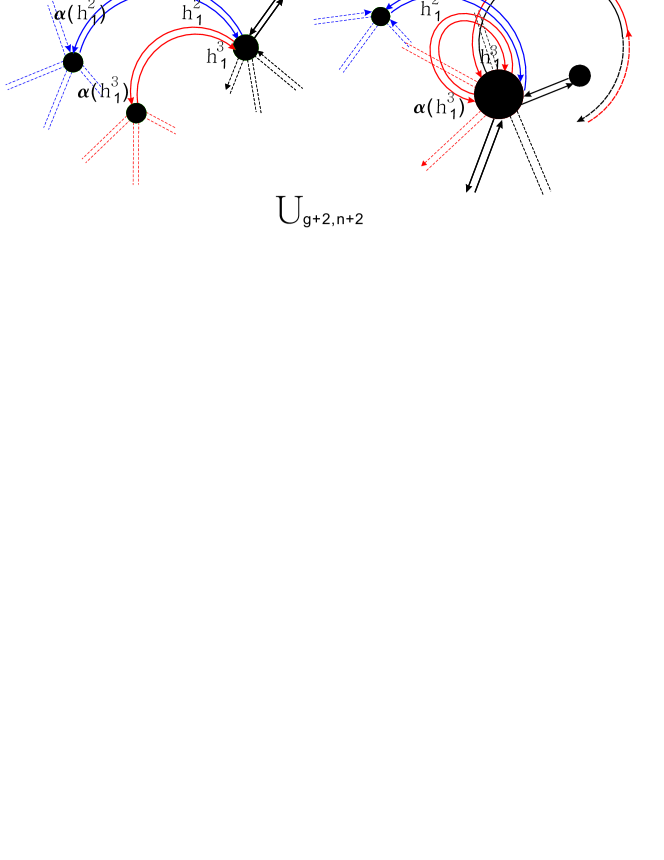
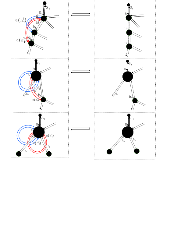
To begin, we consider for $m\geq 3$ the four half edges $h_{1}^{2}$, $\alpha(h_{1}^{2})$, $h_{1}^{3}$ and $\alpha(h_{1}^{3})$. Clearly, $\alpha\circ\sigma(h_{1}^{2})=\alpha(h_{1}^{3})$, whence $h_{1}^{2}<_{\gamma}\alpha(h_{1}^{3})$. Furthermore, by construction,

$$\alpha(h_{1}^{2})<_{\gamma}h_{1}^{2},\quad\alpha(h_{1}^{2})<_{\gamma}h_{1}^{3},\quad h_{1}^{2}<_{\gamma}\alpha(h_{1}^{3}),$$

see also Fig. 2. Accordingly, there are the two scenarios

$$(A)\quad\alpha(h_{1}^{2})<_{\gamma}h_{1}^{2}<_{\gamma}\alpha(h_{1}^{3})<_{\gamma}h_{1}^{3}\quad\text{\rm and}\quad(B)\quad\alpha(h_{1}^{2})<_{\gamma}h_{1}^{3}<_{\gamma}h_{1}^{2}<_{\gamma}\alpha(h_{1}^{3}).$$

The case $m=2$ belongs to scenario $(A)$, which then reduces to

$$\quad\alpha(h_{1}^{2})<_{\gamma}h_{1}^{2}.$$

This generates the bipartition of $U_{g+2,n+2}$,

$$U_{g+2,n+2}=U_{g+2,n+2}^{A}\,\dot{\cup}\,U^{B}_{g+2,n+2}.$$ (3.2)

Lemma 1.

In $U_{g+2,n+2}^{A}$-elements the half-edges $\alpha(h_{1}^{2})$ and $h_{1}^{2}$ belong to two different vertices, $v_{1}$ and $v_{2}$.

Proof.

We have

$$\alpha(h_{1}^{2})<_{\gamma}h_{1}^{2}<_{\gamma}\alpha(h_{1}^{3})<_{\gamma}h_{1}^{3},$$

and $\gamma(\alpha(h_{1}^{2}))=h_{1}^{2}$. Suppose now $\alpha(h_{1}^{2})$ and $h_{1}^{2}$ belong to $v_{1}$. Then there exists a half-edge $k_{i}$ satisfying $\gamma(k_{i})=h_{1}^{2}$ such that $h_{1}^{3}<_{\gamma}k_{i}$ or $h_{1}^{3}=k_{i}$, but this implies $h_{1}^{3}<_{\gamma}h_{1}^{2}$, a contradiction. ∎

We next refine $U^{A}_{g+2,n+2}$: for $u_{g+2,n+2}\in U_{g+2,n+2}^{A}$, we consider the cycle

$$\bar{\gamma}=(\alpha(h_{1}^{2}),2,\ldots,h_{1}^{2},\alpha(h_{1}^{3}),\ldots,h_{1}^{3},h_{1}^{3}+1,\ldots,2(n+1))$$

and we use $(\alpha(h_{1}^{i}),h_{1}^{i}),i=2,3$ to split the $\bar{\gamma}$ into

$$\bar{\gamma}_{1}=(\alpha(h_{1}^{2}),2,\ldots,h_{1}^{2});\quad\bar{\gamma}_{2}=(\alpha(h_{1}^{3}),\ldots,h_{1}^{3});\quad\bar{\gamma}_{3}=(h_{1}^{3}+1,\ldots,2(n+1)),$$ (3.3)

see Fig. 2.

Fig. 2: The three branches (red, blue, black) together with the two pairs $(\alpha(h_{1}^{2}),h_{1}^{2})$ and $(\alpha(h_{1}^{3}),h_{1}^{3})$.

Suppose the restriction $\alpha|_{S}$ is a welldefined fixed-point free involution, then we call $S$ closed. Similarly, the sets $H_{\gamma_{1},\dots,\gamma_{r}}$ and $H_{\bar{\gamma}_{i}}$, $i=1,2,3$ are called closed, if $\alpha|_{H_{\gamma_{1},\dots,\gamma_{r}}}$ and $\alpha|_{H_{\bar{\gamma}_{i}}}$ are fixed-point free involutions.

Let $U_{g+2,n+2}^{II}$ denote the subset of $U^{A}_{g+2,n+2}$-elements in which no $H_{\bar{\gamma}_{i}}$ is closed and let $U_{g+2,n+2}^{I}$ denote its complement. Then

$$U^{A}_{g+2,n+2}=U_{g+2,n+2}^{I}\,\dot{\cup}\,U_{g+2,n+2}^{II}.$$ (3.4)

We refine $U_{g+2,n+2}^{I}$ further:

• $U^{1}_{g+2,n+2}$: the set of $U_{g+2,n+2}^{I}$-elements in which exactly two ${\bar{\gamma}_{i}},{\bar{\gamma}_{j}}$ are empty,

• $U^{2}_{g+2,n+2}$: the set of $U_{g+2,n+2}^{I}$-elements in which exactly one ${\bar{\gamma}_{i}}$ is empty,

• $U^{>2}_{g+2,n+2}$: the complement of $U^{1}_{g+2,n+2}$ and $U^{2}_{g+2,n+2}$, that is, the set of $U_{g+2,n+2}^{I}$ in which no ${\bar{\gamma}_{i}}$ is empty.

Thus

$$U^{I}_{g+2,n+2}=U^{1}_{g+2,n+2}\,\dot{\cup}\,U^{2}_{g+2,n+2}\,\dot{\cup}\,U^{>2}_{g+2,n+2}.$$ (3.5)

We refine $U_{g+2,n+2}^{>2}$ a bit more, for this purpose let

• $U^{>2,3}_{g+2,n+2}$: be the subset of $U_{g+2,n+2}^{>2}$-elements in which $\bar{\gamma}_{1}=(\alpha(h_{1}^{2}),h_{1}^{2})$.

• $U^{>2,4}_{g+2,n+2}$: be the subset of $U_{g+2,n+2}^{>2}$-elements in which $\bar{\gamma}_{1}=(\alpha(h_{1}^{2}),k^{2}_{1},\ldots,k_{1}^{m})$, $m\geq 4$ and $\bar{\gamma}_{2}=(\alpha(h_{1}^{3}),h_{1}^{3})$.

• $U^{5}_{g+2,n+2}$: the complement of $U^{>2,3}_{g+2,n+2}$ and $U^{>2,4}_{g+2,n+2}$, that is subset of $U^{>2}_{g+2,n+2}$-elements in which $\bar{\gamma}_{1}=(\alpha(h_{1}^{2}),k^{2}_{1},\ldots,k_{1}^{m})$ and $\bar{\gamma}_{2}=(\alpha(h_{1}^{3}),k^{2}_{2},\ldots,k_{2}^{l})$, $m,l\geq 4$.

Accordingly,

$$U^{>2}_{g+2,n+2}=U^{5}_{g+2,n+2}\,\dot{\cup}\,U^{>2,3}_{g+2,n+2}\,\dot{\cup}\,U^{>2,4}_{g+2,n+2}.$$ (3.6)

Furthermore we present $U^{>2,3}_{g+2,n+2}$ :

$$U^{>2,3}_{g+2,n+2}=U^{3}_{g+2,n+2}\setminus U^{m,1}_{g+2,n+2},$$ (3.7)

where

• $U^{3}_{g+2,n+2}$ denotes the subset of $U_{g+2,n+2}^{I}$-elements in which $\bar{\gamma}_{1}=(\alpha(h_{1}^{2}),h_{1}^{2})$,

• $U^{m,1}_{g+2,n+2}$ denotes the subset of $U^{2}_{g+2,n+2}$-elements in which $\bar{\gamma}_{1}=(\alpha(h_{1}^{2}),h_{1}^{2})$.

Furthermore we present $U^{>2,4}_{g+2,n+2}$ as

$$U^{>2,4}_{g+2,n+2}=U^{4}_{g+2,n+2}\setminus(U^{m,2}_{g+2,n+2}\,\dot{\cup}\,U^{m,3}_{g+2,n+2}),$$ (3.8)

where

• $U^{4}_{g+2,n+2}$ is the subset of $U_{g+2,n+2}^{I}$-elements with $\bar{\gamma}_{2}=(\alpha(h_{1}^{3}),h_{1}^{3})$,

• $U^{m,2}_{g+2,n+2}$ is the subset of $U^{2}_{g+2,n+2}$-elements with $\bar{\gamma}_{2}=(\alpha(h_{1}^{3}),h_{1}^{3})$,

• $U^{m,3}_{g+2,n+2}$ is the subset of $U^{>2}_{g+2,n+2}$-elements with $\bar{\gamma}_{1}=(\alpha(h_{1}^{2}),h_{1}^{2})$ and $\bar{\gamma}_{2}=(\alpha(h_{1}^{3}),h_{1}^{3})$.

4 Some lemmas

In this section we state three procedures that are employed repeatedly in our bijection. They are “cutting”, “contraction” and “deletion”. These procedures constitute the key three operations that, applied in various contexts, facilitate the bijection.

Lemma 2.

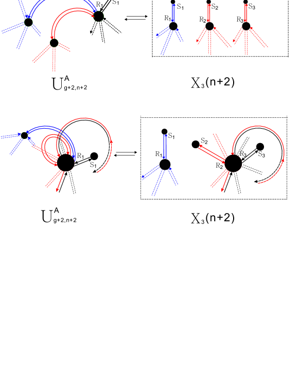
(Cutting) Suppose we are given a planted, unicellular map $u=(H,\alpha,\gamma)\in U^{A}_{g+2,n+2}$ with

$$\gamma=(R_{1},\alpha(h_{1}^{2}),\ldots,h_{1}^{2},\alpha(h_{1}^{3}),\ldots,h_{1}^{3},h_{1}^{3}+1,\ldots,2(n+1),S_{1}).$$ (4.1)

Then $u$ can be mapped to a planted, $3$-cellular map, $x_{3,n+2}\in X_{3}(n+2)$, with the three faces $\gamma_{1},\gamma_{2},\gamma_{3}$ via

$$\begin{split}&c_{2}\colon U^{A}_{g+2,n+2}\longrightarrow X_{3}(n+2),\\ &(H,\alpha,\gamma)\mapsto(H,\alpha,(\gamma_{1},\gamma_{2},\gamma_{3}))\end{split}$$ (4.2)

where

$$\gamma_{1}=(R_{1},1,\ldots,m_{1},S_{1}),\ \gamma_{2}=(R_{2},m_{1}+1,\ldots,m_{2},S_{2}),\ \gamma_{3}=(R_{3},m_{2}+1,\ldots,m_{3},S_{3}).$$ (4.3)

Furthermore, the mapping $c_{2}$ has the following inverse:

$$\begin{split}&g_{2}\colon X_{3}(n+2)\longrightarrow U^{A}_{g+2,n+2}\\ &(H,\alpha,(\gamma_{1},\gamma_{2},\gamma_{3}))\mapsto(H,\alpha,\gamma).\end{split}$$ (4.4)

Proof.

By assumption we have

$$\alpha(h_{1}^{2})<_{\gamma}h_{1}^{2}<_{\gamma}\alpha(h_{1}^{3})<_{\gamma}h_{1}^{3},$$

whence the face of $u_{g+2,n+2}$ can be written as in eq. (4.1). We use $(\alpha(h_{1}^{i}),h_{1}^{i}),i=2,3$ and $\bar{\gamma}_{i},i=1,2,3$ which are given by  3.3, then concatenate the sequence of half-edges of $(R_{1})$, $\bar{\gamma}_{3}$ and $(S_{1})$ to form

$$\begin{split}&\gamma_{1}=\bar{\gamma}_{1},\quad\gamma_{2}=\bar{\gamma}_{2},\quad\\ &\gamma_{3}=(R_{1},h_{1}^{3}+1,\ldots,2(n+1),S_{1})\end{split}$$ (4.5)

and relabel the cycles as in eq. (4.3). This produces the plants $(S_{1})$, $(S_{2})$ and $(S_{3})$. Since $\prod_{i=1}^{3}\gamma_{i}\in S_{2n+2}$, $c_{2}(H,\alpha,\gamma)$ is a $3$-cellular map, $c_{2}$ is well-defined, see Fig. 3.

Fig. 3: The mappings $c_{2}$ and $g_{2}$.

We next construct an explicit inverse of $c_{2}$. Suppose we are given a $3$-cellular map $c_{2}((H,\alpha,\gamma))$, in which the $\gamma_{i}$ are as in eq. (4.5). Then we concatenate the sequences of half-edges of the three $\gamma_{i}$-cycles and relabel as in eq. (4.1), i.e. $\gamma(h_{1}^{2})=\alpha(h_{1}^{3})$, $\gamma(h_{1}^{3})=h_{1}^{3}+1$ and $\gamma(R_{1})=h_{1}^{3}+1$. We derive, by construction,

$$\alpha(h_{1}^{2})<_{\gamma}h_{1}^{2}<_{\gamma}\alpha(h_{1}^{3})<_{\gamma}h_{1}^{3}.$$

Accordingly, $g_{2}(c_{2}(H,\alpha,\gamma))=(H,\alpha,\gamma)$ is a unicellular map of genus $(g+2)$ with property $(A)$. ∎

Lemma 3.

(Contraction) Suppose $u\in U_{g+2,n+2}$ has a one-sided edge $(\alpha(h_{1}^{l_{1}}),h_{1}^{l_{1}})$, $\alpha(h_{1}^{l_{1}})<_{\gamma}h_{1}^{l_{1}}$, such that $\alpha(h_{1}^{l_{1}})$ and $h_{1}^{l_{1}}$ are incident to two different vertices $v_{j},v_{1}$. Relabeling the two half-edges we can write the face

$$\gamma=(R_{1},K_{1},\alpha(h_{1}^{l_{1}}),K_{2},h_{1}^{l_{1}},K_{3},S_{1}).$$ (4.6)

Here either $K_{1}=k_{1}^{1},\ldots,k_{1}^{n_{1}}$ or $K_{1}=\varnothing$, $K_{2}=k_{2}^{1},\ldots,k_{2}^{n_{2}}$ or $K_{2}=\varnothing$ and either $K_{3}=k_{3}^{1},\ldots,k_{3}^{n_{3}}$ or $K_{3}=\varnothing$. Then $u$ corresponds to a unicellular map $u^{\prime}$ together with two distinguished half-edges via mapping

$$\begin{split}&m_{2}\colon U_{g+2,n+2}\longrightarrow U_{g+2,n+1},\\ &((H,\alpha,\gamma),(\alpha(h_{1}^{l_{1}}),h_{1}^{l_{1}}))\mapsto((H^{\prime},\alpha^{\prime},\gamma^{\prime}),(\alpha(h_{1}^{l_{1}})-1,h_{1}^{l_{1}}-1))\end{split}$$ (4.7)

where $H^{\prime}=H\setminus\{h_{1}^{l_{1}},\alpha(h_{1}^{l_{1}})\}$, $\alpha^{\prime}=\alpha\setminus(h_{1}^{l_{1}},\alpha(h_{1}^{l_{1}})$, $\gamma^{\prime}=(R_{1},K_{1},K_{2},K_{3},S_{1})$ and $\alpha(h_{1}^{l_{1}})-1=k_{1}^{n_{1}},h_{1}^{l_{1}}-1=k_{2}^{n_{2}}$, if $K_{1},K_{2}\neq\varnothing$, $\alpha(h_{1}^{l_{1}})-1=h_{1}^{l_{1}}-1=k_{1}^{n_{1}}$, if $K_{1}\neq\varnothing$ and $K_{2}=\varnothing$, $\alpha(h_{1}^{l_{1}})-1=R_{1}$, $h_{1}^{l_{1}}-1=k_{2}^{n_{1}}$, if $K_{1}=\varnothing$ and $K_{2}\neq\varnothing$, and finally $\alpha(h_{1}^{l_{1}})=h_{1}^{l_{1}}=R_{1}$, if $K_{1},K_{2}=\varnothing$.
Furthermore the mapping $e_{2}$

$$\begin{split}&e_{2}\colon U_{g+2,n+1}\longrightarrow U_{g+2,n+2},\\ &((H^{\prime},\alpha^{\prime},\gamma^{\prime}),(\alpha(h_{1}^{l_{1}})-1,h_{1}^{l_{1}}-1))\mapsto((H,\alpha,\gamma),(\alpha(h_{1}^{l_{1}}),h_{1}^{l_{1}}))\end{split}$$ (4.8)

has the property $e_{2}\circ m_{2}=\text{\rm id}$.

Proof.

$m_{2}((H,\alpha,\gamma),(\alpha(h_{1}^{l_{1}}),h_{1}^{l_{1}}))$ is by construction unicellular and retains the genus of $(H,\alpha,\gamma)$. ∎

We describe the contraction in Fig. 4.

Fig. 4: The mappings $m_{2}$ and $e_{2}$. The edge $(\alpha(h_{1}^{l_{1}}),h_{1}^{l_{1}})$ (green) is one-sided edge.

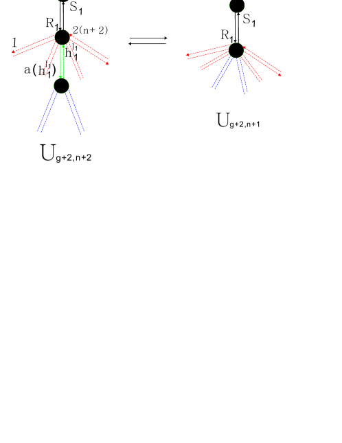
Lemma 4.

(Deletion) Given a unicellular map $u=(H,\alpha,\gamma)\in U_{g+2,n+2}^{B}$ with face

$$\gamma=(R_{1},\alpha(h_{1}^{2}),K_{1},h_{1}^{3},K_{2},h_{1}^{2},\alpha(h_{1}^{3}),K_{3},S_{1}),$$ (4.9)

where $K_{1}=k_{1}^{1},\ldots,k_{1}^{n_{1}}$ or $K_{1}=\varnothing$, $K_{2}=k_{2}^{1},\ldots,k_{2}^{n_{2}}$ or $K_{2}=\varnothing$ and $K_{3}=k_{3}^{1},\ldots,k_{3}^{n_{3}}$ or $K_{3}=\varnothing$.
Then $u$ corresponds to a unicellular map $u^{\prime}=(H^{\prime},\alpha^{\prime},\gamma^{\prime})\in U_{g+1,n}$ together with two half-edges $k_{l_{1}}$ and $k_{l_{2}}$, where $k_{l_{1}}\leq_{\gamma}k_{l_{2}}$, via the mapping

$$\begin{split}&r_{2}\colon U^{B}_{g+2,n+2}\longrightarrow U_{g+1,n}\\ &((H,\alpha,\gamma))\mapsto((H^{\prime},\alpha^{\prime},\gamma^{\prime}),(k_{l_{1}},k_{l_{2}})),\end{split}$$ (4.10)

where $H^{\prime}=H\setminus\{\alpha(h_{1}^{2}),h_{1}^{2},\alpha(h_{1}^{3}),h_{1}^{3}\}$, $\alpha^{\prime}=\alpha\setminus\{(h_{1}^{2},\alpha(h_{1}^{2})),(h_{1}^{3},\alpha(h_{1}^{3}))\}$ and

$$\gamma^{\prime}=(R_{1},K_{2},K_{1},K_{3},S_{1}).$$ (4.11)

$r_{2}$ can be reversed by mapping a unicellular map $u=(H,\alpha^{\prime},\gamma^{\prime})$, together with two arbitrary half-edges $k_{l_{1}}$ and $k_{l_{2}}$ ($k_{l_{1}}<_{\gamma}k_{l_{2}}$) as follows:

$$\begin{split}&s_{2}\colon U_{g+1,n}\longrightarrow U^{B}_{g+2,n+2}\\ &((H^{\prime},\alpha^{\prime},\gamma^{\prime}),(k_{l_{1}},k_{l_{2}}))\mapsto(H,\alpha,\gamma).\end{split}$$ (4.12)

Proof.

By construction $\gamma^{\prime}\in S_{2(n-2)}$, $\alpha^{\prime}$ is a fixed-point free involution and $H^{\prime}$ has cardinality $2(n-2)$, whence $r_{2}((H,\alpha,\gamma))$ is unicellular. Euler characteristic implies that the genus of $r_{2}((H,\alpha,\gamma))$ is $(g-1)$. Moreover, we have in case of $K_{1},K_{2}\neq\varnothing$, $k_{l_{1}}=k_{1}^{n_{1}},k_{l_{2}}=k_{2}^{n_{2}}$, in case of $K_{1}\neq\varnothing$ $K_{2}=\varnothing$, $k_{l_{1}}=k_{l_{2}}=k_{1}^{n_{1}}$, in case of $K_{1}=\varnothing$ and $K_{2}\neq\varnothing$, $k_{l_{1}}=R_{1}$, $k_{l_{2}}=k_{2}^{n_{1}}$, and in case of $K_{1},K_{2}=\varnothing$ we have $k_{l_{1}}=k_{l_{2}}=R_{1}$, see Fig. 5.

Fig. 5: The mappings $r_{2}$ and $s_{2}$. The deleting edges are $(\alpha(h_{1}^{2}),h_{1}^{2})$ (blue) and $(\alpha(h_{1}^{3}),h_{1}^{3})$ (red). The gray dotted lines denote a sequence of half-edges connecting two vertices.

Given a unicellular map $(H^{\prime},\alpha^{\prime},\gamma^{\prime})\in U_{g+1,n}$, there are

$${2n+1\choose 2}+{2n+1\choose 1}=\frac{(2n+1)(2n)}{2}+2n+1=(2n+1)(n+1)$$

ways to choose $(k_{l_{1}},k_{l_{2}})$ such that $k_{l_{1}}<_{\gamma}k_{l_{2}}$. We now select two half-edges $(k_{l_{1}},k_{l_{2}})$ such that $k_{l_{1}}<_{\gamma}k_{l_{2}}$ and insert the pairs of half-edges $(\alpha(h_{1}^{i}),h_{1}^{i})$, $i=2,3$ into the face $\gamma^{\prime}$. This produces the face $\gamma$, with $\gamma(R_{1})=\alpha(h_{1}^{2})$, $\gamma(k_{l_{2}})=h_{1}^{2}$, $\gamma(k_{l_{1}})=h_{1}^{3}$ and $\gamma(h_{1}^{2})=\alpha(h_{1}^{3})$, $\gamma(h_{1}^{3})=\gamma^{\prime}(R_{1})$ and $\gamma(\alpha(h_{1}^{3}))=\gamma^{\prime}(k_{l_{2}})$. Consequently we have

$$\gamma=(R_{1},\alpha(h_{1}^{2}),\ldots,k_{l_{1}},h_{1}^{3},\ldots,k_{l_{2}},h_{1}^{2},\alpha(h_{1}^{3}),\ldots,S_{1}).$$

We then relabel $\gamma$ as in eq. (4.9). Since $\alpha$ is a fixed-point free involution and $H$ is a set of cardinality $2(n+2)$, $s_{2}(H^{\prime},\alpha^{\prime},\sigma^{\prime})$ is a unicellular map with property $B$. Euler characteristic implies $s_{2}(H^{\prime},\alpha^{\prime},\sigma^{\prime})$ has genus $(g+2)$. By construction, we have $s_{2}\circ r_{2}=id_{U_{g+2,n+2}^{B}}$. ∎

5 The main theorem

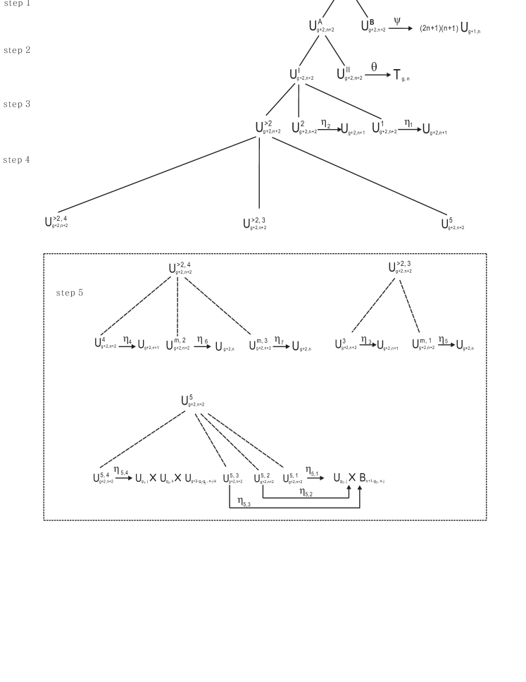
In this section we state some auxiliary bijections and our main result. We furthermore give in Fig. 6 an modular description of how our bijection works.

We call a planted $2$-cellular map, whose combinatorial graph is connected, a planted, bicellular map. Let $B_{g,n}$ denote the set of planted, bicellular maps of genus $g$ with $n$ $(np)$-edges.

Let $U^{5,i}_{g+2,n+2}$ denote the subset of $U^{5}_{g+2,n+2}$ in which only a single $H_{\bar{\gamma}_{i}}$, $i=1,2,3$ is closed and let $U_{g+2,n+2}^{5,4}$ denote the set of $U^{5}_{g+2,n+2}$-elements in which all $H_{\bar{\gamma}_{i}}$, $i=1,2,3$ are closed, i.e. $U^{5}_{g+2,n+2}=\dot{\cup}_{i=0}^{4}U^{5,i}_{g+2,n+2}$.

Lemma 5.

We have the bijections

$$\eta_{5,i}\colon U^{5,i}_{g+2,n+2} \longrightarrow \dot{\bigcup}_{0\leq g_{3}\leq g+1,\;0\leq j,k\leq n}\left(U_{g_{3},j}\times B_{g+1-g_{3},n-j}\right),\quad 1\leq i\leq 3;$$

$$\eta_{5,4}\colon U^{5,4}_{g+2,n+2} \longrightarrow \bigcup_{0\leq g_{1},g_{2}\leq g+2,\;0\leq j,k\leq n}U_{g_{1},j}\times U_{g_{2},k}\times U_{g+2-g_{1}-g_{2},n-j-k}.$$

We prove Lemma 5 in Section 6.

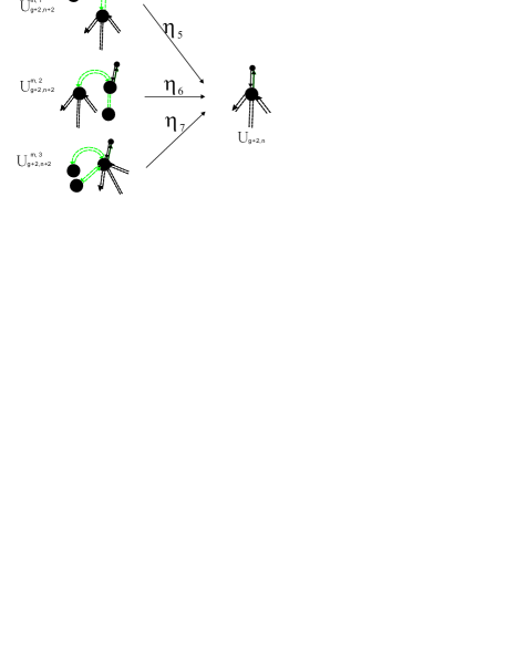
Lemma 6.

There are fours bijections, $\eta_{i}$ for $i=1,\ldots,4$,

$$\eta_{1}\colon U^{1}_{g+2,n+2}\longrightarrow U_{g+2,n+1}.$$

$$\eta_{2}\colon U^{2}_{g+2,n+2}\longrightarrow U_{g+2,n+1}.$$

$$\eta_{3}\colon U^{3}_{g+2,n+2}\longrightarrow U_{g+2,n+1}.$$

$$\eta_{4}\colon U^{4}_{g+2,n+2}\longrightarrow U_{g+2,n+1}.$$

We prove Lemma 6 in Section 6.

Lemma 7.

We have the three bijections:

$$\eta_{5}\colon U^{m,1}_{g+2,n+2}\longrightarrow U_{g+2,n}.$$

$$\eta_{6}\colon U^{m,2}_{g+2,n+2}\longrightarrow U_{g+2,n}.$$

$$\eta_{7}\colon U^{m,3}_{g+2,n+2}\longrightarrow U_{g+2,n}.$$

We prove Lemma 7 in Section 6.

A planted $3$-cellular map that is connected as a combinatorial graph is called a planted tri-cellular map. Let $T_{g,n}$ denote the set of planted, tricellular maps of genus $g$ with $n$ $(np)$-edges.

Proposition 1.

There is a bijection

$$\theta\colon U^{II}_{g+2,n+2}\longrightarrow T_{g,n}.$$

We prove Proposition 1 in Section 6.

Proposition 2.

There is a bijection

$$\psi\colon U^{B}_{g+2,n+2}\longrightarrow(2n+1)(n+1)U_{g+1,n}.$$

We prove Proposition 1 in Section 6. In Figure 6 we give an overview of how the above bijections are applied.

Fig. 6: Applying the bijections.

For a set $A^{\xi}_{g,n}$ we denote its cardinality by ${\sf a}^{\xi}_{g}(n)$.

Theorem 1.

$$\begin{split}&{\sf u}_{g+2}(n+2)=\\ &{\sf t}_{g}(n)+{\sf d}_{g+2}(n)+4{\sf u}_{g+2}(n+1)-3{\sf u}_{g+2}(n)+(n+1)(2n+1){\sf u}_{g+1}(n),\end{split}$$ (5.1)

where

$$\begin{split}&{d}_{g+2}(n)=\\ &3\sum_{g_{1}=0}^{g+1}\sum_{0\leq m\leq n}\,{\sf u}^{*}_{g_{1}}(m){\sf b}_{g+1-g_{1}}(n-m)+\sum_{g_{1}}\sum_{g_{2}}\sum_{m_{1}\geq 0}\sum_{m_{2}\geq 0}{\sf u}^{*}_{g_{1}}(m_{1}){\sf u}^{*}_{g_{2}}(m_{2}){\sf u}^{*}_{g+2-g_{1}-g_{2}}(n-m_{1}-m_{2}),\end{split}$$

with

$${\sf u}^{*}_{g}(n)=\begin{cases}0,\quad for\quad g=0\quad and\quad n=0;\\ {\sf u}_{g}(n),\quad otherwise.\end{cases}$$ (5.2)

6 Proofs

Proof of Lemma 5

Proof.

Claim $1$: The mapping

$$\begin{split}&\eta_{5,1}\colon U^{5,1}_{g+2,n+2}\longrightarrow\dot{\bigcup}_{0\leq g_{3}\leq g+1,\;0\leq j,k\leq n}\left(U_{g_{3},j}\times B_{g+1-g_{3},n-j}\right),\\ &u_{g+2,n+2}\mapsto(u_{g_{3},j},b_{g+1-g_{3},n-j}),\quad 0\leq g_{3}\leq g+1,1\leq j\leq n\end{split}$$

is a bijection. We first prove that $\eta_{5,1}$ is welldefined. For a planted unicellular map $(H,\alpha,\gamma)=u_{g+2,n+2}\in U^{5,1}_{g+2,n+2}$ with face

$$\gamma=(R_{1},\alpha(h_{1}^{2}),\ldots,h_{1}^{2},\alpha(h_{1}^{3}),\ldots,h_{1}^{3},h_{1}^{3}+1,\ldots,2(n+1),S_{1}),$$

we employ the mapping $c_{2}$ of the Cutting-Lemma (Lemma 2) in order to decompose $u_{g+2,n+2}$ into a planted $3$-cellular map, $x_{3,n+2}=(H,\alpha,(\gamma_{i})_{1\leq i\leq 3})$, where

$$\begin{split}&\gamma_{1}=\bar{\gamma}_{1},\quad\gamma_{2}=\bar{\gamma}_{2},\quad\\ &\gamma_{3}=(R_{1},h_{1}^{3}+1,\ldots,2(n+1),S_{1}),\end{split}$$ (6.1)

where $\gamma_{3}$ is obtained by concatenating the sequence of half-edges of $(R_{1})$, $\bar{\gamma}_{3}$ and $(S_{1})$.

For any $(H,\alpha,\gamma)=u_{g+2,n+2}\in U^{5,1}_{g+2,n+2}$, $H_{\bar{\gamma}_{1}}$ is closed. Since $\gamma_{1}=\bar{\gamma}_{1}$, the restriction $\alpha|_{H_{\gamma_{1}}}$ is a fixed-point free involution. Accordingly, $(H_{\gamma_{1}},\alpha|_{H_{\gamma_{1}}},\gamma_{1})$ is a planted unicellular map.

Since $H_{\bar{\gamma}_{2}}\cup H_{\bar{\gamma}_{3}}$ is closed and $\gamma_{i}$, $i=2,3$ is given in eq. (6.1), the restriction $\alpha|_{H_{\gamma_{1},\gamma_{2}}}$ is a welldefined fixed-point free involution. Furthermore, since neither $H_{\bar{\gamma}_{2}}$ nor $H_{\bar{\gamma}_{3}}$ are closed, $H_{\gamma_{2}}$ and $H_{\gamma_{3}}$ are not closed either. Therefore $(H_{\gamma_{1},\gamma_{2}},\alpha|_{H_{\gamma_{1},\gamma_{2}}},(\gamma_{i})_{1\leq i\leq 2})$ is a planted bicellular map with the plants $(S_{1})$ and $(h_{1}^{3})$.

Let $u_{g_{3},j}=(H_{\gamma_{1}},\alpha|_{H_{\gamma_{1}}},\gamma_{1})$ and $b_{g^{\prime},n^{\prime}}=(H_{\gamma_{1},\gamma_{2}},\alpha|_{H_{\gamma_{1},\gamma_{2}}},(\gamma_{i})_{1\leq i\leq 2})$.

Suppose $u_{g+2,n+2}$, $u_{g_{3},j}$ and $b_{g^{\prime},n^{\prime}}$ have $J$, $J_{\gamma_{1}}$ and $J_{b}$ vertices, respectively. Then $2-2(g+2)=J-(n+2)+1$ and $2-2g_{3}=J_{\gamma_{1}}-j+1$, whence

$$2-2(g+1-g_{3})=J-J_{\gamma_{1}}-(n-j)+2.$$

Since the edges incident to plants and plants do not contribute to the number of edges and vertices, we have $n^{\prime}=n-j,1\leq j\leq n$, $J_{b}=J-J_{\gamma_{1}}$. As a result $b_{g^{\prime},n^{\prime}}$ has genus $(g+1-g_{3})$, where $0\leq g_{3}\leq g+1$, whence $\eta_{5,1}$ is welldefined.

We next show that $\eta_{5,1}$ is injective. In order to apply the mapping $c_{2}$ of the Cutting-Lemma, we introduce

$$\begin{split}&\zeta_{5,1}((H_{\gamma_{1}},\alpha|_{H_{\gamma_{1}}},\gamma_{1}),(H_{\gamma_{1},\gamma_{2}},\alpha|_{H_{\gamma_{1},\gamma_{2}}},(\gamma_{i})_{1\leq i\leq 2}))=(H,\alpha,(\gamma_{i})_{1\leq i\leq 3}),\end{split}$$ (6.2)

where $\gamma_{i}$ are given by eq. (6.1), $\alpha=\alpha|_{H_{\gamma_{1},\gamma_{2},\gamma_{3}}}$ and $H=H_{\gamma_{1}}\cup H_{\gamma_{1},\gamma_{2}}$.

For any

$$\eta_{5,1}((H,\alpha,\gamma))=(u_{g_{3},j},b_{g+1-g_{3},n-j})\in\dot{\bigcup}_{0\leq g_{3}\leq g+1,\;0\leq j,k\leq n}\left(U_{g_{3},j}\times B_{g+1-g_{3},n-j}\right),$$

where $u_{g_{3},j}=(H_{\gamma_{1}},\alpha|_{H_{\gamma_{1}}},\gamma_{1})$, and $b_{g+1-g_{3},n-j}=(H_{\gamma_{1},\gamma_{2}},\alpha|_{H_{\gamma_{1},\gamma_{2}}},(\gamma_{i})_{1\leq i\leq 2})$, we apply $\zeta_{5,1}$. This generates the $3$-cellular map $(H,\alpha,(\gamma_{i})_{1\leq i\leq 3})$. Since $u_{g_{3},j}$ has $j$ edges and $b_{g+1-g_{3},n-j}$ has $(n-j)$ edges, and the process generates the edges $(\alpha(h_{1}^{2}),h_{1}^{2})$ and $(\alpha(h_{1}^{3}),h_{1}^{3})$, we have $x_{3,n+2}=(H,\alpha,(\gamma_{i})_{1\leq i\leq 3})\in X_{3}(n+2)$. We can now apply $c_{2}$ of Lemma 2, which induces the mapping $c_{5,1}\colon X_{3}(n+2)\longrightarrow U^{5,1}_{g+2,n+2}$. Lemma 2 now implies furthermore

$$(c_{5,1}\circ\zeta_{5,1})\circ\eta_{5,1}=\text{\rm id},$$

whence the mapping $\eta_{5,1}$ is injective.

It thus remains to prove that $\eta_{5,1}$ is surjective. This follows again from close inspection of the proof of the Lemma 2, which implies

$$\eta_{5,1}\circ(c_{5,1}\circ\zeta_{5,1})=\text{\rm id}.$$

Therefore, $\eta_{5,1}$ is surjective and Claim $1$ is completed.

Analogously we prove that $\eta_{5,2}$ and $\eta_{5,3}$ are injective.

Claim $2$: The mapping

$$\begin{split}&\eta_{5,4}:U^{5,4}_{g+2,n+2}\longrightarrow\bigcup_{0\leq g_{1},g_{2}\leq g+2,\;0\leq j,k\leq n}U_{g_{1},j}\times U_{g_{2},k}\times U_{g+2-g_{1}-g_{2},n-j-k},\\ &u_{g+2,n+2}\mapsto(u_{g_{1},j},u_{g_{2},k},u_{g+2-g_{1}-g_{2},n-j-k}),\end{split}$$

with $1\leq g_{1},g_{2}\leq g+2$ and $1\leq j,k\leq n$ is a bijection.

We first show that $\eta_{5,4}$ is well-defined. As in the proof of Claim $1$, we employ the Cutting-Lemma which produces a $3$-cellular map with the boundary components $(\gamma_{1},\gamma_{2},\gamma_{3})$.

For any $u_{g+2,n+2}\in U^{5,4}_{g+2,n+2}$, each of the $H_{\bar{\gamma}_{i}}$ is closed. Thus the restrictions $\alpha|_{H_{\gamma_{i}}}$, for $i=1,2,3$ are welldefined and fixed-point free involutions. As a result, $(H_{\gamma_{1}},\alpha|_{H_{\gamma_{1}}},\gamma_{1})$, $(H_{\gamma_{1}},\alpha|_{H_{\gamma_{2}}},\gamma_{2})$ and $(H_{\gamma_{1}},\alpha|_{H_{\gamma_{3}}},\gamma_{3})$ are unicellular maps, respectively.

Let $u_{g_{1},j}=(H_{\gamma_{1}},\alpha|_{H_{\gamma_{1}}},\gamma_{1})$, $u_{g_{2},k}=(H_{\gamma_{2}},\alpha|_{H_{\gamma_{2}}},\gamma_{2})$ and $u_{g^{\prime},n^{\prime}}=(H_{\gamma_{3}},\alpha|_{H_{\gamma_{3}}},\gamma_{3})$. Suppose that $u_{g+2,n+2}$, $u_{g_{1},j}$, $u_{g_{2},k}$ and $u_{g^{\prime},n^{\prime}}$ have $J$, $J_{\gamma_{1}}$, $J_{\gamma_{2}}$ and $J_{\gamma_{3}}$ vertices, respectively. Then

$$2-2(g+2)=J-(n+2)+1,\quad 2-2g_{1}=J_{\gamma_{1}}-j+1,\quad\text{and}\quad 2-2g_{2}=J_{\gamma_{2}}-k+1,\quad 1\leq j,k\leq n.$$ (6.3)

Furthermore, we have

$$\begin{split}&J-J_{\gamma_{1}}-J_{\gamma_{2}}-(n-j-k)+1=2-2(g+2-g_{1}-g_{2}).\end{split}$$

After applying the Cutting-Lemma, $(h_{1}^{2})$ and $(h_{1}^{3})$ become plants, similarly $(\alpha(h_{1}^{2}),h_{1}^{2})$ and $(\alpha(h_{1}^{3}),h_{1}^{3})$ become edges incident to plants. Thus, we have $n^{{}^{\prime}}=n-j-k,0\leq j,k\leq n$ and $J_{\gamma_{3}}=J-2-J_{\gamma_{1}}-J_{\gamma_{2}}$ and accordingly obtain

$$\begin{split}&J-2-J_{\gamma_{1}}-J_{\gamma_{2}}-(n-j-k)+1=2-2(g+2-g_{1}-g_{1}).\end{split}$$

Consequently, $u_{g^{{}^{\prime}},n^{{}^{\prime}}}$ has genus $(g+2-g_{1}-g_{2})$, where $0\leq g_{1},g_{2}\leq g+2$ and $\eta_{5,4}$ is well-defined.

We next prove $\eta_{5,4}$ is injective. We establish this as in Claim $1$, introducing

$$\begin{split}&\zeta_{5,4}:((H_{\gamma_{1}},\alpha|_{H_{\gamma_{1}}},\gamma_{1}),(H_{\gamma_{2}},\alpha|_{H_{\gamma_{2}}},\gamma_{2}),(H_{\gamma_{3}},\alpha|_{H_{\gamma_{3}}},\gamma_{3}))\mapsto(H,\alpha,(\gamma_{i})_{1\leq i\leq 3})\\ \end{split}$$ (6.4)

where $\gamma_{i}$ is given in eq. (6.1), $\alpha=\alpha|_{H_{\gamma_{1},\gamma_{2},\gamma_{3}}}$ and $H=H_{\gamma_{1}}\cup H_{\gamma_{1},\gamma_{2}}$. Analogously, $c_{2}$ of Lemma 2 induces the mapping $c_{5,4}$ and

$$(c_{5,4}\circ\zeta_{5,4})\circ\eta_{5,4}=\text{\rm id},$$

whence the mapping $\eta_{5,4}$ is injective.

Subjectivity of $\eta_{5,4}$ is implied by the Cutting-Lemma which guarantees

$$\eta_{5,4}\circ(c_{5,4}\circ\zeta_{5,4})=\text{\rm id},$$

whence Claim $2$ and the proof of the lemma is complete. ∎

Proof of Proposition 1.

Proof.

We prove that the mapping

$$\begin{split}&\theta\colon U^{II}_{g+2,n+2}\longrightarrow T_{g,n},\\ &u_{g+2,n+2}\mapsto t_{g,n}\end{split}$$ (6.5)

is a bijection. As for welldefinedness, suppose $u_{g+2,n+2}\in U^{II}_{g+2,n+2}$ where

$$\gamma=(R_{1},\alpha(h_{1}^{2}),\ldots,h_{1}^{2},\alpha(h_{1}^{3}),\ldots,h_{1}^{3},h_{1}^{3}+1,\ldots,2(n+1),S_{1}).$$

We use mapping $c_{2}$ of the Cutting-Lemma and derive the planted $3$-cellular map, $x_{3,n+2}=(H,\alpha,(\gamma_{i})_{1\leq i\leq 3})$, where

$$\begin{split}&\gamma_{1}=\bar{\gamma}_{1},\quad\gamma_{2}=\bar{\gamma}_{2},\quad\\ &\gamma_{3}=(R_{1},h_{1}^{3}+1,\ldots,2(n+1),S_{1}).\end{split}$$ (6.6)

Here $\gamma_{3}$ is obtained by concatenating the sequence of half-edges contained in $(R_{1})$, $\bar{\gamma}_{3}$ and $(S_{1})$.

For $u_{g+2,n+2}\in U^{II}_{g+2,n+2}$ none of the $H_{\bar{\gamma}_{i}}$, $i=1,2,3$ is closed, whence the associated combinatorial graph of $x_{3,n+2}$ is connected. Accordingly, $x_{3,n+2}=\theta(u_{g+2,n+2})$ is a planted tricellular map with plants $(h_{1}^{2})$, $(h_{1}^{3})$ and $(S_{1})$. Euler’s characteristic formula implies $t_{g,n}$ has genus $g$ and $n$ edges, whence $\theta$ is well-defined. Injectivity and surjectivity of $\theta$ are implied by the Cutting Lemma. ∎

Proof of Lemma 6.

Proof.

Claim $1$: The mapping

$$\begin{split}&\eta_{1}\colon U^{1}_{g+2,n+2}\longrightarrow U_{g+2,n+1},\\ &((H,\alpha,\gamma),(\alpha(h_{1}^{2}),h_{1}^{2}))\mapsto((H^{\prime},\alpha^{\prime},\gamma^{\prime}),(\alpha(h_{1}^{2})-1,h_{1}^{2}-1)).\end{split}$$ (6.7)

is a bijection.

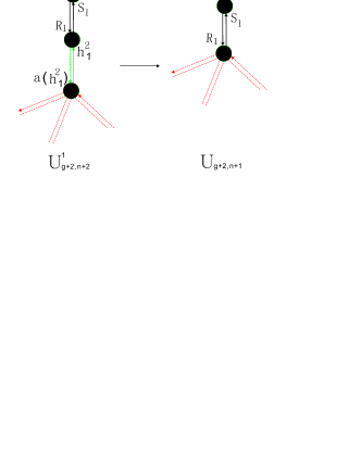
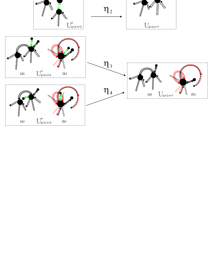
The contraction lemma implies that $\eta_{1}$ is welldefined. Injectivity of $\eta_{1}$ follows by considering the mapping $\rho_{1}$ induced by the mapping $e_{2}$ of Lemma 3, where $\rho_{1}((H^{\prime},\alpha^{\prime},\gamma^{\prime}))=(H,\alpha,\gamma)\in U^{1}_{g+2,n+2}$. Lemma 3 guarantees $\rho_{1}\circ\eta_{1}=\text{\rm id}$, whence $\eta_{1}$ is injective. Surjectivity of $\eta_{1}$ is a consequence of $\eta_{1}\circ\rho_{1}=id$, implied by Lemma 3, see Fig. 7.

Fig. 7: The mapping $\eta_{1}$ and the one-sided edge $(\alpha(h_{1}^{2}),h_{1}^{2}))$ (green).

The proof that $\eta_{j}\colon U^{j}_{g+2,n+2}\longrightarrow U_{g+2,n+1}$ is a bijection for $j=2,3,4$ follows analogously, see Fig. 8.

Fig. 8: The mappings $\eta_{2}$, $\eta_{3}$ and $\eta_{4}$.

∎

The proof of Lemma 7.

Proof.

Claim $1$: The mapping

$$\begin{split}&\eta_{5}\colon U^{m,1}_{g+2,n+2}\longrightarrow U_{g+2,n},\\ &((H,\alpha,\gamma),(\alpha(h_{1}^{2}),h_{1}^{2}),(\alpha(h_{1}^{3}),h_{1}^{3}))\mapsto((H^{\prime},\alpha^{\prime},\gamma^{\prime}),(\alpha(h_{1}^{2})-1,h_{1}^{2}-1),(\alpha(h_{1}^{3})-1,h_{1}^{3}-1))\end{split}$$ (6.8)

is a bijection.

We first prove that $\eta_{5}$ is welldefined. Consider $(H,\alpha,\gamma)\in U^{m,1}_{g+2,n+2}$ together with two one-sided edges, $(\alpha(h_{1}^{2}),h_{1}^{2})$, $(\alpha(h_{1}^{3}),h_{1}^{3})$, such that $h_{1}^{1}$ and $h_{1}^{2}$ are incident to $v_{1}$, $\alpha(h_{1}^{1})$ and $\alpha(h_{1}^{2})$ are incident to $v_{i}$ and $v_{j}$.

We then apply Lemma 3 to a $(H,\alpha,\gamma)\in U^{m,1}_{g+2,n+2}$ together with the one-side edge $(\alpha(h_{1}^{2}),h_{1}^{2})$. We iterate applying Lemma 3 w.r.t. the edge $(\alpha(h_{1}^{3}),h_{1}^{3})$. By definition of Lemma 3 this generates the unicellular map $(H^{\prime},\alpha^{\prime},\gamma^{\prime})$ of genus $(g+2)$ having $n$ edges with distinguished four half-edges $\alpha(h_{1}^{2})-1$, $h_{1}^{2}-1$, $\alpha(h_{1}^{3})-1$ and $h_{1}^{3}-1$.

Since Lemma 3 preserves genus, $\eta_{5}((H,\alpha,\gamma))$ has genus $(g+2)$ and $n$ edges, whence $\eta_{5}$ is well-defined.

We next prove $\eta_{5}$ is injective. Suppose we have a unicellular map $(H^{\prime},\alpha^{\prime},\gamma^{\prime})\in U_{g+2,n}$ with four distinguished half-edges $\alpha(h_{1}^{2})-1$, $h_{1}^{2}-1$, $\alpha(h_{1}^{3})-1$ and $h_{1}^{3}-1$. We observe that the mapping $m_{2}$ constructed in Lemma 3 allows us to obtain a mapping $\rho_{5}\colon U_{g+2,n}\to U^{m,1}_{g+2,n+2}$ such that

$$\rho_{5}\circ\eta_{5}=\text{\rm id},$$

whence injectivity.

Surjectivity follows by computing $\eta_{5}\circ\rho_{5}=\text{\rm id}$.

The proof that

$$\eta_{6}\colon U^{m,2}_{g+2,n+2}\longrightarrow U_{g+2,n}\quad\text{\rm and}\quad\eta_{7}\colon U^{m,3}_{g+2,n+2}\longrightarrow U_{g+2,n}$$

are bijections is analogous, see Fig. 9.

Fig. 9: The mappings $\eta_{5}$, $\eta_{6}$ and $\eta_{7}$.

∎

The proof of Proposition 2.

Proof.

Proposition 2 follows directly from Lemma 4. ∎

The proof of Theorem 1.

Proof.

According to Lemma 5, Lemma 6, Lemma 7, Proposition 1 and Proposition 2, we have

• ${\sf u}_{g+2}^{0,i}(n+2)={\sf u}_{g+2}(n+1)$, for $1\leq i\leq 4$,

• ${\sf u}^{i}_{g+2}(n+2)={\sf u}_{g+2}(n+1)$, for $1\leq i\leq 4$,

• ${\sf u}^{m,j}_{g+2}(n+2)={\sf u}_{g+2}(n)$, for $1\leq j\leq 3$,

• ${\sf u}^{II}_{g+2}(n+2)={\sf t}_{g}(n)$,

• ${\sf u}^{B}_{g+2}(n+2)=(n+1)(2n+1){\sf u}_{g+1}(n)$.

According to eq. (3.2), eq. (3.4) and eq. (3.5) we have

$$\begin{split}&{\sf u}_{g+2,n+2}\\ =&{\sf u}^{I}_{g+2}(n+2)+{\sf u}^{II}_{g+2}(n+2)+{\sf u}^{B}_{g+2}(n+2)\\ =&1+2{\sf u}_{g+2}(n+1)+{\sf u}^{>2}_{g+2}(n+2))+{\sf t}_{g}(n)+(n+1)(2n+1){\sf u}_{g+1}(n).\end{split}$$ (6.9)

Furthermore, according to eq. (3.6), eq. (3.7) and eq. (3.8), we have

$$\begin{split}&{\sf u}^{>2}_{g+2}(n+2)\\ =&{\sf u}^{5}_{g+2}(n+2)+{\sf u}^{>2,3}_{g+2}(n+2)+{\sf u}_{g+2}^{>2,4}(n+2)\\ =&{\sf d}_{g+2}(n)+2{\sf u}_{g+2}(n+1)-3{\sf u}_{g+2}(n),\end{split}$$ (6.10)

which establishes eq. (5.1). ∎

7 Acknowledgments.

Many thanks to our group at SDU for discussions and suggestions. We furthermore acknowledge the financial support of the Future and Emerging Technologies (FET) programme within the Seventh Framework Programme (FP7) for Research of the European Commission, under the FET-Proactive grant agreement TOPDRIM, number FP7-ICT-318121.

References

- [1] J.E. Andersen, R.C. Penner, C.M. Reidys, and F.W.D. Huang. Topology of RNA-RNA interaction structures. J. Comput. Biol., 19(7), 928–943, 2012.
- [2] J.E. Andersen, R.C. Penner, C.M. Reidys, and M.S. Waterman. Topological classification and enumeration of RNA structures by genus. J. Math. Biol., 2012.
- [3] F. Dyson. The s matrix in quantum electrodynamics. Phys. Rev., 75, 1736, 1949.
- [4] G. Chapuy. A new combinatorial identity for unicellular maps, via a direct bijective approach. Adv. Appl. Math., 47(4), 874-893, 2011.
- [5] H.S.W. Han and C.M. Reidys. A bijection between unicellular and bicellular maps. arXiv:1301.7177.
- [6] T.J.X. Li and C.M. Reidys. Combinatorics of RNA-RNA interaction. Math. Biosc., (233), 1, 47-58, 2011.
- [7] M. Loebl and I. Moffatt. The chromatic polynomial of fatgraphs and its categorification. Adv. Math., 217, 1558-1587, 2008.
- [8] R. C. Penner. The Teichmuller space of a punctured surface. Comm. Math. Phys., 1987.
- [9] R. C. Penner. Perturbative series and the moduli space of Riemann surfaces. J. Differential Geom., 27(1), 35-53, 1988.
- [10] R. C. Penner and M. S. Waterman. Spaces of RNA secondary structures. Adv. Math., 101, 31-49, 1993.
- [11] B. E. Sagan. The Symmetric Group: Representations, Combinatorial Algorithms, and Symmetric Functions. Springer-Verlag, New York, 2001.
- [12] J. Schwinger. On Green’s functions of quantized fields I+II. Proc. Natl. Acad. Sci, 37, 452-459, 1951.
- [13] J. Harer and D. Zagier. The Euler characteristic of the moduli space of curves. Invent. Math., 85, 457-485, 1986.
- [14] D. Zagier. On the distribution of the number of cycles of elements in symmetric groups. Nieuw Arch. Wiskd., IV. Ser., 13(3), 489-495, 1995.