On differentially dissipative dynamical systems
Abstract
Dissipativity is an essential concept of systems theory. The paper provides an extension of dissipativity, named differential dissipativity, by lifting storage functions and supply rates to the tangent bundle. Differential dissipativity is connected to incremental stability in the same way as dissipativity is connected to stability. It leads to a natural formulation of differential passivity when restricting to quadratic supply rates. The paper also shows that the interconnection of differentially passive systems is differentially passive, and provides preliminary examples of differentially passive electrical systems.
keywords:
Dissipativity, incremental stability, contraction analysis,
1 Introduction
Dissipativity, Willems (1972a); Willems (1972b), plays a central role in the analysis of open systems to reduce the analysis of complex systems to the study of the interconnection of simpler components. Dissipativity is a fundamental tool in nonlinear control design Sepulchre et al. (1997); van der Schaft (1999), widely adopted in industrial applications. Typical examples are provided by applications on electro-mechanical devices modeled within the port-hamiltonian framework, Ortega et al. (2001). Passivity-based designs conveniently connect the physical modeling of mechanical and electrical interconnections and the stability properties required by applications.
In a nonlinear setting, applications like regulation, observer designs, and synchronization call for incremental notions of stability, Angeli (2000); Angeli (2009). Several results in the literature propose extensions of passivity to guarantee connections to incremental properties. For example, in the theory of equilibrium independent passivity, Hines et al. (2011); Jayawardhana et al. (2007), the dissipation inequality refers to pairs of system trajectories, one of which is a fixed point. The incremental passivity of Desoer and Vidyasagar (1975) and Stan and Sepulchre (2007) characterizes a passivity property of solutions pairs, through the use of incremental storage functions reminiscent of the notion of incremental Lyapunov functions of Angeli (2000), and supply rates of the form , for and , where and refers to input/output signals.
Incremental passivity is equivalent to passivity for linear systems. It has been used in nonlinear control for regulation, Pavlov and Marconi (2008), and synchronization purposes, Stan and Sepulchre (2007). Yet, it requires the construction of a storage function in the extended space of paired solutions, a difficult task in general, and the a priori formulation of the supply rate based on the difference between signals, which does not take into account the possible nonlinearities of the state and external spaces. A motivation for the present work partly come A motivation for the present paper partly comes from the role of incremental properties in ant windup design of induction motors Sepulchre et al. (2011) and the difficulty to establish those properties in models that integrate magnetic saturation, see Example 5.2 in the present paper.
A different approach to the characterization of incremental properties is provided by contraction, a differential concept The theory developed in Lohmiller and Slotine (1998) recognizes that the infinitesimal approximation of a system carries information about the behavior of its solutions set. It provides a variational approach to incremental stability, based on the linearization of the system, without explicitly constructing the distance measuring the convergence of solutions towards each other.
Following this basic idea, the present paper proposes a dissipativity theory based on the infinitesimal variations of dynamical systems along their solutions. We call it differential dissipativity because it is classical dissipativity lifted to the tangent bundle of the system manifold. In analogy with the classical relation between storage functions and Lyapunov functions, the proposed notion of differential storage function for differential dissipativity is paired to the notion of Finsler-Lyapunov function recently proposed in Forni and Sepulchre (2012), which plays a role in connecting differential dissipativity and incremental stability. The preprint van der Schaft (2013) is an insightful complementary effort in that direction, connecting the framework to the early concept of prolonged system in nonlinear control Crouch and van der Schaft (1987).
The are many potential advantages in developing a differential version of dissipativity theory. First of all, differential dissipativity is equivalent to dissipativity for linear systems. In the nonlinear setting, the fact that the infinitesimal approximation of a nonlinear system is a linear time-varying system opens the way to a characterization of differential passivity - differential dissipativity with quadratic supply rates - that falls in the linear setting of Willems (1972b). Moreover, differential dissipativity provides an input-output characterization of the dynamical system in the infinitesimal neighborhood of each trajectory, which leads to state-dependent differential supply rates. This is of relevance to tailor the dissipativity property to nonlinear state and external variables spaces.
The content of the paper is developed in analogy with classical results on dissipativity. The instrumental notion of displacement dynamical system is provided in Section 2. Differential dissipativity and differential passivity are formulated in Sections 3 and 4, Examples of differentially passive electromechanical systems are proposed in Section 5. Conclusion follows. Proofs are in appendix. This paper is an extended version of Forni and Sepulchre (2013).
Notation. The exposition of the differential dissipativity approach is developed on manifolds following the notation of Absil et al. (2008) and Do-Carmo (1992).
Given a manifold , and a point of , denotes the tangent space of at . is the tangent bundle. Given two manifolds and and a mapping . is of class , , if the function is of class , where and are smooth charts. The differential of at is denoted by . A curve on a given manifold is a mapping . For simplicity we sometime use or to denote . Specifically, this notation is adopted when the variable in refers to time.
is the identity matrix of dimension . Given a vector , denotes the transpose vector of . Given a matrix we say that or if or , for each , respectively. Given the vectors , . A locally Lipschitz function is said to belong to class if it is strictly increasing and ; it belongs to class if, moreover, .
A distance (or metric) on a manifold is a positive function that satisfies if and only if , for each and for each . If but we say that is a pseudo-metric. A set is bounded if for any given distance on . A curve is bounded when its image is bounded. Given a manifold , a set of isolated points satisfies: for any distance function on and any given pair in , there exists an such that . Given and , the composition assigns to each the value . Given a function , the matrix of partial derivatives is denoted as (Jacobian). denotes the Hessian of .
2 Displacement dynamical systems
Taking inspiration from the dissipativity paper of Willems (1972a) and from the (state-space) behavioral framework in Willems (1991), given smooth manifolds and , a time-invariant dynamical system is represented by algebraic-differential equations of the form
| (1) |
where , , is the state, and collects the external variables. The behavior of is given by the set of absolutely continuous curves that satisfy for (almost) all . Given , - input, - output, and , we say that is a solution to (1) from the initial condition under the action of the input .
In what follows we assume that are functions. When the external variables are organized into input and output variables, i.e. , we also assume existence, unicity, and forward completeness of solutions for each initial condition and input . Note that under mild regularity assumptions on , if , every is a curve, as clarified in Chapter IV, Section 4, of Boothby (2003).
Under these assumptions, the displacement dynamical system induced by is represented by
| (2a) | |||||
| (2b) | |||||
and it is given by the set of curves that satisfy (2) for each .
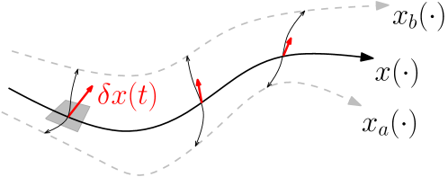
Following the interpretation proposed in Lohmiller and Slotine (1998), given a point , a tangent vector represents an infinitesimal variation - or displacement - on . In this sense characterizes the infinitesimal difference between every two neighborhood solutions, that is, the infinitesimal variations on the solutions to (1). A graphical representation of a displacement is proposed in Figure 1. The intuitive notion of infinitesimal variation is made precise in Remark 2.1.
Remark 2.1
For each , consider a (parameterized) curve . We assume that . An infinitesimal variation on is given by . As a matter of fact, for each . In fact, by chain rule111The differential in the right-hand side of the first identity refers to the mapping from to . The one in the right-hand side of the second identity refers to the mapping from to .,
| (3) |
where the third identity follows from the fact that is a function, by assumption (in local coordinates .
When the manifold is equipped with a Finsler metric (see, for example, Tamássy (2008); Bao et al. (2000)), the time-evolution of along the solutions to (2) measures the contraction of the dynamical system , that is, the tendency of solutions to converge towards each other. The connection between the displacement dynamical system and incremental stability properties have been exploited in the seminal paper of Lohmiller and Slotine (1998), and in many other works, e.g. Lewis (1949); Aghannan and Rouchon (2003); Pavlov et al. (2004); Wang and Slotine (2005); Fromion and Scorletti (2005); Pham and Slotine (2007); Russo et al. (2010). A unifying framework for contraction based on the extension of Lyapunov theory to the tangent bundle has been recently proposed in Forni and Sepulchre (2012).
3 Differentially dissipative systems
We develop the theory of differential dissipativity mimicking classical dissipativity, Willems (1972a); Sepulchre et al. (1997); van der Schaft (1999). In analogy to the intuitive interpretation of a storage function as the energy of the system, it is convenient to view the differential storage function as the infinitesimal energy associated to the infinitesimal variation on a given solution . This energy can be either increased or decreased through the supply provided by external sources, as prescribed by a differential supply rate .
Definition 3.1
Consider a manifold and a set of isolated points . For each , consider a subdivision of into a vertical distribution
| (4) |
and a horizontal distribution complementary to , i.e. , given by
| (5) |
where , , and , , are vector fields.
A function is a differential storage function for the dynamical system in (1) if there exist , , and such that
| (6) |
for all , where and satisfies the following conditions:
-
(i)
and are functions for each and ;
-
(ii)
and satisfy and for each such that , , and .
-
(iii)
for each and .
-
(iv)
for each , , and ;
-
(v)
for each and such that and (strict convexity).
Definition 3.2
The function provides a non-negative value to each . When , a suggestive notation for is - a non-symmetric norm on each tangent space - which immediately connects the differential storage to the idea of an energy of the displacement , since . From Definition 3.1 it is possible to identify differential storage functions and horizontal Finsler-Lyapunov functions , introduced in Section VIII of Forni and Sepulchre (2012). Therefore the existence of a differential storage endows with the structure of a pseudo-metric space, which plays a central role in connecting differential dissipativity to incremental stability. Restricting a differential storage to horizontal distributions is convenient in many situations where contraction takes place only in certain directions. For example, let be the state space and suppose that the output is given by where is a differentiable function. Then, in coordinates, is a possible candidate storage function with horizontal distribution given by the span of the columns of the matrix . With this storage, the state-space becomes a pseudo-metric space, while the output space becomes a metric space. Further details are collected in Remark 3.3.
Remark 3.3
Suppose that for each , , and take . Then, is a Finsler structure on (see, for example, Tamássy (2008); Bao et al. (2000)). Then, we can define the length of a curve as . The induced distance between any two points is given by , where is the set of piecewise curves in such that and . For the case , we have the identity , where the function projects every tangent vector into . In this case, measures only the horizontal contribution of , and the induced , is only a pseudo-distance on , since for some . An extended discussion and examples are provided in Sections IV and VIII of Forni and Sepulchre (2012).
We can finally provide the definition of differential dissipativity. We emphasize that differential dissipativity is just dissipativity lifted to the tangent bundle.
Definition 3.4
Exploiting the assumption , (8) is equivalent to
| (9) |
We conclude the section by illustrating a first connection between differential dissipativity and incremental stability.
Theorem 3.5
Suppose that the dynamical system represented by (1) is differentially dissipative with differential storage and differential supply rate . Suppose also that for , - input, - output, it holds that for each , and each . Then, there exists a class function such that
| (10) |
for each and each , such that , where is the pseudo-distance induced by , with degree of homogeneity of (see Definition 3.1).
Note that if , then is a distance on , thus Theorem 3.5 guarantees that is incrementally stable for any feedforward input signal .
4 Differential passivity
Following the approach of Willems (1972b), we formulate differential passivity as the restriction of differential dissipativity to quadratic supply rates. To this end, we consider the external variable manifold as the product of an input vector space and an output vector space such that . A consequence of working with a vector space is that for each . In what follows, we will use to denote the input and to denote the output.
For each , let be a -tensor field on that provides an inner product on each tangent space , denoted by . For simplicity of the exposition, we write to denote , or to denote .
Definition 4.1
For each , let be a -tensor field on . A dynamical system is differentially passive if it is differentially dissipative with respect to a differential supply rate of the form
| (11) |
is uniformly differentially passive whenever is independent on . Finally, we say that is strictly differentially passive if there exists a function of class such that (9) is restricted to .
As in passivity, the next theorems show that the feedback interconnection of differentially passive systems is differentially passive.
Theorem 4.2
Let and be (strictly) uniformly differentially passive dynamical systems. Suppose that and that their supply rates are based on the same -tensor . Then, the dynamical system arising from the feedback interconnection
| (12) |
is (strictly) uniformly differentially passive from to .
Theorem 4.3
Let and be (strictly) differentially passive dynamical systems. Suppose that and that their supply rates are based on the -tensors for and for , respectively. Then, the dynamical system arising from the feedback interconnection
| (13) |
is differentially passive from to , provided that
| (14) |
for each and each .
The state-feedback interconnection in (13) is in contrast with the classical passivity approach that looks at systems as input/output operators. However, differently from classical passivity and from uniform differential passivity, differential passivity is an input/output characterization of the system that depends on the trajectories, geometrically expressed by a different tensor for each . This lack of uniformity with respect to the solutions of the system requires extra-effort at interconnection, as shown by (14). In this sense, the key role of the state-feedback (13) is to equalize the two tensors and , to achieve the desired interconnected behavior. Despite the state dependence, Theorem 4.3 can be conveniently used for design.
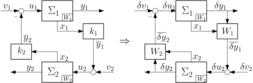
Example 4.4
Consider the dynamical system of equations
| (15) |
whose induced displacement dynamical system is represented by (15) and
| (16) |
Let a symmetric matrix for each . is differentially passive with differential supply rate if there exist a matrix , where , and an invertible matrix such that
| (17) |
In fact, define . Then,
| (18) |
Example 4.5
Consider the dynamical system given by
| (19) |
whose displacement dynamics is given by
| (20) |
Let a symmetric matrix for each . is differentially passive with differential supply rate if there exists a matrix , where , such that
| (21) |
for each and . In fact, using the differential storage , we get
| (22) |
Example 4.6
Consider two systems and satisfying (17) respectively with matrices and , and constant matrices and . The closed-loop system given by the feedback interconnection (13) is differentially passive provided that
| (23) |
This is an immediate consequence of Theorem 4.3, since
| (24) |
as required by (14). A graphical interpretation of (23) is provided in Figure 2.

We conclude the section by extending Theorem 3.5. The next theorem shows that a differentially passive dynamical system with “excess” of output differential passivity behaves like a filter: its steady-state output depends only on the signal at the input.
Theorem 4.7
Let be a differentially passive dynamical system with
-
•
differential storage such that for each ;
-
•
differential supply rate such that for each and each (excess of output passivity).
Let be a input signal and suppose that every curve remains bounded.
Then, for any pair ,
| (25) |
The hypothesis of the theorem guarantees incremental stability of - a consequence of Theorem 3.5. If is strictly differentially passive, then Theorem 4.7 can be strengthened towards incremental asymptotic stability. Finally, the case of is not taken into account here but it presents similarities with the analysis of Section 2.3.2 in Sepulchre et al. (1997), about passivity with semidefinite storage functions and stability.
5 Examples of differentially passive electrical circuits
In the first example below we show the differential passivity of a simple nonlinear RC circuit. Differential passivity is also used in the second example below to develop an feed-forward control strategy for an induction motor with flux saturations.
Example 5.1 (Nonlinear RC circuit)
Consider the simple circuit reproduced in Figure 3. The nonlinearity of the circuit is due to the nonlinear relation between the charge and the voltage of the capacitor. We suppose that is differentiable and strictly increasing.
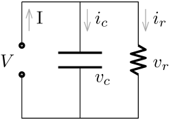
The algebraic-differential description of the circuit is given by the constitutive relations of each component and by Kirchhoff laws,
| (26) |
Following (2), the displacement dynamical systems is thus represented by (26) and by the set of equations
| (27) |
The circuit is differentially passive from to with differential storage . In fact, define , then
| (28) |
where the last identity follows from the fact that is greater than 0 for each value of , and .
Example 5.2 (Induction motor with flux saturation)
We revisit the model proposed in Sullivan et al. (1996). The model is developed in a rotating frame at speed . The rotor speed is denoted by . Rotor and stator magnetic flux vectors are denoted respectively by and . Rotor and stator currents are given by and . The analysis below takes into account only the electrical part of the motor. The mechanical equations are thus not detailed. Indeed, for , the differential relations are given by
| (29a) | |||||
| (29b) | |||||
| (29c) | |||||
where , and and are rotor and stator resistances. is the (disturbance) load, and is a control input. The motor model is completed by the algebraic relations between currents and fluxes, given by
| (30) |
, , and are the usual inductances adopted in classical linear flux-current models, while the nonlinear functions and characterize the flux saturation. For instance, satisfies a relation of the form where is a monotonically increasing sector function, that is, and , for each . These assumptions guarantee that
| (31) |
Indeed, the current may grow faster than the flux (for ), which characterizes a limited increase of the flux despite large increments of the currents. Similar assumptions hold for . Note that the alignment of current and flux vectors is preserved.
In what follows we will use to denote the dynamical system represented by (29) and (30). Using and , is given by the set of curves that satisfy (29) and (30) for each .
The analysis proposed below is based on the introduction of a new dynamical system, the virtual dynamical system (see, for example, Wang and Slotine (2005)), represented by (29b), (29c) and (30), where the relation between the rotor speed and the flux is disregarded. To distinguish between the induction motor and the associated virtual system, we use over-lined variables: and . Indeed, for each , is the virtual dynamical system given by the set of curves that satisfy (29b), (29c) and (30) (expressed in the over-lined variables).
The crucial relation between and the virtual system is that if , then . Exploiting this relation, it is possible to infer properties of from the properties of the virtual dynamical system .
For the virtual system , and are exogenous signal acting uniformly on each solution . Therefore for both and one can consider (see Remark 2.1). The virtual displacement dynamical system is thus given by (29b), (29c) and (30) (expressed in the over-lined variables) and by
| (32) |
| (33) |
(32) and (33) characterize respectively a differentially passive dynamical system and a differentially passive static nonlinearity. For (32), consider the differential storage . Then,
| (34) |
which establish uniform differential passivity from to of the dynamical system represented by (29b), (29c) (expressed in the over-lined variables).
On the other hand, for (33) we get
| (35) |
From (34) and (35), the combination of (32) and (33) guarantees that is strictly uniformly differentially passive from to , for each . In fact,
| (36) |
where is the quantity between brackets in (35). Because , for (feedforward signal), Theorem 4.7 guarantees that
| (37) |
for all , in Note that the boundedness of these curves is guaranteed for bounded signals by the combination of the effect of the dissipative terms in (32) and the alignment between currents and fluxes in (33).
The incremental property (37) of the virtual system can be used to provide an feedforward control design for . For illustration purposes, in what follows we consider the goal of asymptotically regulate towards a prescribed flux configuration .
From (37), achieving the goal for the virtual system is straightforward: if then each curve satisfies . Indeed, from (29b), (29c), and (30), the feedforward input given by
| (38) |
guarantees that .
The reader will notice that for any given selection of , with given in (38), the curve belongs to . This is a consequence of the fact that is formulated by taking into account explicitly and . Thus, exploiting the fact that if , then , we can conclude that
| (39) |
for all with in (38). A similar (but dynamic) design of can be provided for the regulation of to .
6 Conclusions
The concept of differential dissipativity is introduced as a natural extension of differential stability for open systems. The differential storage is inspired from the Finsler-Lyapunov function of Forni and Sepulchre (2012) and has the interpretation of (infinitesimal) energy of a displacement along a solution curve through . Extending the role of dissipativity theory for analysis and design of interconnections in the tangent bundle offers a novel way to study incremental stability (or contraction) properties of nonlinear systems.
Appendix A Proofs
Proof of Theorem 3.5 [Sketch]. In accordance with Remark 2.1, we can consider curves in for . In fact, for any given pair of curves , the associated parameterization satisfies , that is, for each and .
As a consequence, by differential dissipativity, we have . Because the differential storage is also a non-increasing horizontal Finsler-Lyapunov function, (10) is a consequence of Theorem 3 in Forni and Sepulchre (2012) Moreover, the case of differential storages with , is a consequence of Theorem 1 in Forni and Sepulchre (2012).
Proof of Theorem 4.2 Define the differential storage 222When clear from the context, we drop the arguments of the functions to simplify the notation.. The functions and below must be set to zero for the weaker property of uniform differential passivity.
| (40) |
where . In fact,
| (41) |
where the first inequality follows from the definition of , and the last inequality holds because (i) for ; (ii) for ; (iii) and .
Note that characterizes an inner product on the product manifold .
Proof of Theorem 4.3 Define the differential storage . As in the proof of Theorem 4.2, and below must be set to zero for the case of differential passivity.
| (42) |
For each point of the product manifold , defines a -tensor on the product manifold .
Proof of Theorem 4.7. Let be any pair of curves in . For each , define , and consider a (parameterized) curve such that and . We assume that .
For each , define
| (43) |
Repeating the argument of Remark 2.1, one can show that is a solution to (2) from the initial condition under the action of the input . Thus, the storage function satisfies
| (44) |
By boundedness of , define a compact set such that for each and each . depends on the range of , and on the range of parameterization of the curve . The compactness of guarantees the existence of a smooth -tensor field such that
| (45) |
for each . Then,
| (46) |
that is,
| (47) |
By Barbalat’s lemma, for each ,
| (48) |
The applicability of Barbalat’s lemma follows from the fact that is uniformly continuous for each . In fact, the range of is bounded for each . This is a consequence of the fact that each curve to is bounded and that . Therefore, for each , belongs to a compact subset of that depends on the initial condition and on the input . Thus, for each , is uniformly continuous, since it is a function on a compact set.
References
- Absil et al. (2008) P.-A. Absil, R. Mahony, and R. Sepulchre. Optimization Algorithms on Matrix Manifolds. Princeton University Press, Princeton, NJ, 2008. ISBN 978-0-691-13298-3.
- Aghannan and Rouchon (2003) N. Aghannan and P. Rouchon. An intrinsic observer for a class of lagrangian systems. IEEE Transactions on Automatic Control, 48(6):936 – 945, 2003. ISSN 0018-9286.
- Angeli (2000) D. Angeli. A Lyapunov approach to incremental stability properties. IEEE Transactions on Automatic Control, 47:410–421, 2000.
- Angeli (2009) D. Angeli. Further results on incremental input-to-state stability. IEEE Transactions on Automatic Control, 54(6):1386–1391, 2009.
- Bao et al. (2000) D. Bao, S.S. Chern, and Z. Shen. An Introduction to Riemann-Finsler Geometry. Springer-Verlag New York, Inc. (2000), 2000. ISBN ISBN 0-387-98948-X.
- Boothby (2003) W.M. Boothby. An Introduction to Differentiable Manifolds and Riemannian Geometry, Revised. Pure and Applied Mathematics Series. Acad. Press, 2003. ISBN 9780121160517.
- Crouch and van der Schaft (1987) P.E. Crouch and A.J. van der Schaft. Variational and Hamiltonian control systems. Lecture notes in control and information sciences. Springer, 1987. ISBN 9783540183723.
- Desoer and Vidyasagar (1975) C.A. Desoer and M. Vidyasagar. Feedback Systems: Input-Output Properties, volume 55 of Classics in Applied Mathematics. Society for Industrial and Applied Mathematics, 1975. ISBN 9780898716702.
- Do-Carmo (1992) M.P. Do-Carmo. Riemannian Geometry. Birkhäuser Boston, 1992. ISBN 0817634908.
- Forni and Sepulchre (2012) F. Forni and R. Sepulchre. A differential Lyapunov framework for contraction analysis. Submitted to IEEE Transactions on Automatic Control., 2012.
- Forni and Sepulchre (2013) F. Forni and R. Sepulchre. On differentially dissipative dynamical systems. In 9th IFAC Symposium on Nonlinear Control Systems, 2013.
- Fromion and Scorletti (2005) V. Fromion and G. Scorletti. Connecting nonlinear incremental Lyapunov stability with the linearizations Lyapunov stability. In 44th IEEE Conference on Decision and Control, pages 4736 – 4741, December 2005.
- Hines et al. (2011) G.H. Hines, M. Arcak, and A.K. Packard. Equilibrium-independent passivity: A new definition and numerical certification. Automatica, 47(9):1949 – 1956, 2011. ISSN 0005-1098.
- Jayawardhana et al. (2007) B. Jayawardhana, R. Ortega, E. García-Canseco, and F. Castaños. Passivity of nonlinear incremental systems: Application to PI stabilization of nonlinear rlc circuits. Systems and Control Letters, 56(9-10):618–622, 2007.
- Lewis (1949) D. C. Lewis. Metric properties of differential equations. American Journal of Mathematics, 71(2):294–312, April 1949.
- Lohmiller and Slotine (1998) W. Lohmiller and J.E. Slotine. On contraction analysis for non-linear systems. Automatica, 34(6):683–696, June 1998. ISSN 0005-1098.
- Ortega et al. (2001) R. Ortega, A.J. Van Der Schaft, I. Mareels, and B. Maschke. Putting energy back in control. Control Systems, IEEE, 21(2):18 –33, apr 2001. ISSN 1066-033X.
- Pavlov and Marconi (2008) A. Pavlov and L. Marconi. Incremental passivity and output regulation. Systems and Control Letters, 57(5):400 – 409, 2008. ISSN 0167-6911.
- Pavlov et al. (2004) A. Pavlov, A. Pogromsky, N. van de Wouw, and H. Nijmeijer. Convergent dynamics, a tribute to Boris Pavlovich Demidovich. Systems & Control Letters, 52(3-4):257 – 261, 2004. ISSN 0167-6911. DOI: 10.1016/j.sysconle.2004.02.003.
- Pham and Slotine (2007) Q.C. Pham and J.E. Slotine. Stable concurrent synchronization in dynamic system networks. Neural Networks, 20(1):62 – 77, 2007. ISSN 0893-6080.
- Russo et al. (2010) G. Russo, M. Di Bernardo, and E.D. Sontag. Global entrainment of transcriptional systems to periodic inputs. PLoS Computational Biology, 6(4):e1000739, 04 2010. 10.1371/journal.pcbi.1000739.
- Sepulchre et al. (1997) R. Sepulchre, M. Jankovic, and P. Kokotovic. Constructive nonlinear Control. Springer Verlag, 1997.
- Sepulchre et al. (2011) R. Sepulchre, T. Davos, F. Jadot, and F. Malrait. Antiwindup design for induction motor control in the field weakening domain. IEEE Transaction on Control Systems Technology, PP(99):1–15, 2011.
- Stan and Sepulchre (2007) G.B. Stan and R. Sepulchre. Analysis of interconnected oscillators by dissipativity theory. Automatic Control, IEEE Transactions on, 52(2):256 –270, feb. 2007. ISSN 0018-9286.
- Sullivan et al. (1996) C.R. Sullivan, Chaofu Kao, B.M. Acker, and S.R. Sanders. Control systems for induction machines with magnetic saturation. IEEE Transactions on Industrial Electronics, 43(1):142 –152, 1996. ISSN 0278-0046.
- Tamássy (2008) L. Tamássy. Relation between metric spaces and Finsler spaces. Differential Geometry and its Applications, 26(5):483 – 494, 2008. ISSN 0926-2245. 10.1016/j.difgeo.2008.04.007.
- van der Schaft (1999) A.J. van der Schaft. -Gain and Passivity in Nonlinear Control. Springer-Verlag New York, Inc., Secaucus, N.J., USA, second edition, 1999. ISBN 1852330732.
- van der Schaft (2013) A.J. van der Schaft. On differential passivity. In 9th IFAC Symposium on Nonlinear Control Systems, 2013.
- Wang and Slotine (2005) W. Wang and J.E. Slotine. On partial contraction analysis for coupled nonlinear oscillators. Biological Cybernetics, 92(1):38–53, 2005.
- Willems (1972a) J.C. Willems. Dissipative dynamical systems part I: General theory. Archive for Rational Mechanics and Analysis, 45:321–351, 1972a. ISSN 0003-9527.
- Willems (1972b) J.C. Willems. Dissipative dynamical systems part II: Linear systems with quadratic supply rates. Archive for Rational Mechanics and Analysis, 45:352–393, 1972b. ISSN 0003-9527.
- Willems (1991) J.C. Willems. Paradigms and puzzles in the theory of dynamical systems. IEEE Transactions on Automatic Control, 36(3):259–294, 1991.