A nonlinear relativistic approach to mathematical representation of vacuum electromagnetism based on extended Lie derivative

Abstract

This paper presents an alternative relativistic nonlinear approach to the vacuum case of classical electrodynamics. Our view is based on the understanding that the corresponding differential equations should be dynamical in nature. So, they must represent local energy-momentum balance relations. Formally, the new equations are in terms of appropriately extended Lie derivative of $\mathbb{R}^{2}$-valued differential 2-form along a $\mathbb{R}^{2}$-valued 2-vector on Minkowski space-time.

1 Introduction

In [1] we presented an alternative view and developed corresponding formal prerelativistic approach to description of time dependent electromagnetic fields in vacuum. Our approach was based on the general view that no point-like and spatially infinite physical objects may exist at all, so the point-like directed idealization of Coulomb law and the D’Alembert wave equation directed idealization of vacuum fields we put on reconsideration. Such a view on physical objects, in particular, on free electromagnetic ones, as spatially finite entities with internal dynamical structure, made us try to work out a new look at the problem of choosing appropriate mathematical images for their physical and dynamical appearances, in general, and for their time stable and recognizable subsystems, in particular, during their existence. In other words, accepting the view for available internal local dynamical structure of free electromagnetic objects, to try to understand in what way and in what extent this internal dynamical structure determines the behavior of these objects as a whole under appropriate invironment. The assumed by us viewpoint there could be shortly characterised in prerelativestic terms as follows.

Time-stability of a free electromagnetic object requires at least two interacting subsystems, and these two subsystems can NOT be formally identified by the electric and magnetic fields $(\mathbf{E},\mathbf{B})$, for example: the first - by $\mathbf{E}$, and the second - by $\mathbf{B}$, because a recognizable subsystem of a propagating electromagnetic physical object must be able to carry momentum, and neither $\mathbf{E}$ nor $\mathbf{B}$ are able to do this separately: the local momentum is $\frac{1}{c}\mathbf{E}\times\mathbf{B}$. The supposed two subsystems might be formally identified in terms of the very $(\mathbf{E},\mathbf{B})$ and, if needed, making use of their derivatives. In order to come to a more adequate formal representatives of these two subsystems we paid due respect to the object that represents formally the physical nature and appearence of an electromagnetic object. For such mathematical object we chose the corresponding Maxwell stress tensor $M(\mathbf{E},\mathbf{B})$. Such a choice was based on the general view that the surviving flexability of any physical object is determined by its capabilities to act upon and to withstand external action upon, so the corresponding theoretical quantities describing the corresponding abilities in our case must have the sense of admissible changes of $M(\mathbf{E},\mathbf{B})$. This understanding directed our attention to the well known formal differential identity satisfied by $M(\mathbf{E},\mathbf{B})$, and brought us to the mathematical images of the two recognizable subsystems, to the differential relations describing their time stability, and to the special interaction respect these two subsystems pay to each other.

Going back to the subject of the present paper we note that after the deep studies of Lorentz [2], Poincare [3] and Einstein [4], the final step towards formal relativisation of Maxwell electrodynamical equations we due to H.Minkowski [5], who explicitly introduced the new mathematics: local view on the space $M=(\mathbb{R}^{4},\eta)$ where $\eta$ is pseudometric tensor field, the classical electric and magnetic vector fields as constituents of a differential 2-form $F$, Maxwell equations in terms of $F$ on $M$, appropriate 4-dimensional extension of Maxwell stress tensor, unifying in this way the concepts of stress, energy and momentum as components af a symmetric 2-tensor field on $M$, and representing the corresponding local conservation laws as zero-divergence of this tensor field.

Later on it was found that Maxwell equations presuppose in fact two differential 2-forms, $(F,*F)$, where $*$ is the Hodge star operator defined by the pseudometric $\eta$ on $\mathbb{R}^{4}$. Moreover, the prerelativistic Maxwell system of equations in the vacuum case was represented in terms of the exterior derivative $\mathbf{d}$ in the form: $\mathbf{d}F=0,\mathbf{d}*F=0$. This form of the equations stabilized strongly during the following years the belief in the 4-potential guage view: the basic mathematical representative of the field should be $u(1)$-valued 1-form $A=A_{\mu}dx^{\mu}\otimes e$ defined on the Minkowski space-time, where $e$ denotes a basis of the 1-dimensional Lie algebra $u(1)$. This view suggested to consider the 2-form $F$ as $\mathbf{d}A$, to call it field strength, but it also reduced the equation $\mathbf{d}F=0$ to trivial and non - informative one. As for the other 2-form $*F$, its non-guage originated differential $\mathbf{d}*F$ was kept in order to be equalized to the electric current 3-form $*j$: $\mathbf{d}*F=*j$. This final relation we can not admit as sufficiently realistic, since mathematics requires on both sides of $"="$ to stay the same quantity, and theoretical physics could hardly present a physical quantity that could be equally well presented by $\mathbf{d}*F$ and by $*j$ in view of their quite different qualitative nature. Nevertheless, this formal view clearly suggests that, from physical point of view, the electromagnetic field should be considered as built of two interacting and recognizable subsystems formally represented by $F$ and $*F$. However, such a view, somehow, was not adopted and further elaborated.

We must note that this relativistic formulation does not introduce new solutions. Moreover, the new form of the equations and the new formal identity satisfied by the relativistically extended Maxwell stress tensor, which was called stress-energy-momentum tensor $Q_{\mu}^{\nu}$, do not introduce explicitly anything about possible nonzero local energy-momentum exchange between the above mentioned two subsystems formally represented by $F$ and $*F$ (see the next section). In this sense, the essential moments of the old viewpoint on the field dynamics were kept unchanged, a serious physical interpretation of $F$ and $*F$ as two physically interacting time-recognizable subsystems, guaranteing time-stability of an electromagnetic field object considered as spatially propagating and spatially finite entity carrying dynamical structure, was not given. In our view, such interpretation is still not sufficiently well understood today and considered as necessary, also, the null field nature of the stress-energy-momentum tensor $Q_{\mu}^{\nu}:Q_{\mu\nu}Q^{\mu\nu}=0$, according to us, is not appropriately appreciated, correspondingly respected, and effectively used.

In this paper we give corresponding to our view relativisation of [1] making use of modern differential geometry and extending appropriately the Lie derivative of differential forms along multivector fields [12] to derivative of vector valued differential forms $\Phi=\Phi^{j}\otimes k_{j}\in\Lambda(M,E_{1})$ along vector valued multivector fields $T=T_{i}\otimes e^{i}\in\mathfrak{X}(M,E_{2})$ with respect to appropriately defined bilinear map $\varphi:E_{1}\times E_{2}\rightarrow F$. The role of $\varphi$ is to recognize and partially evaluate algebraically and differentially the time-stable subsystems represented formally by the components $T_{i}$ of $T$ and $\Phi_{j}$ of $\Phi$, and to separate corresponding interacting couples $(\Phi^{j},T_{i})$.

2 Our basic views

We start with some general remarks.

First, under physical object/system, we understand a system $\mathcal{A}$ of recognizable and spatially finite mutually supporting subsystems through energy exchange physical processes, some of these processes are among the subsystems of $\mathcal{A}$, called by us internal with respect to $\mathcal{A}$, e.g., energy exchange between $F$ and $*F$ in electrodynamics, otherwise, we call them external with respect to $\mathcal{A}$, e.g., electric/gravitational field of a charged/mass particle .

Second, the frequently used in literature concept of physical system in vacuum, we understand as physical system in appropriate media and available appropriate mutual interaction between the object and the media, quaranteeng corresponding time stability and admissible changes of both, the object and the media.

In view of the above, for electromagnetic field objects we assume:

1. Every electromagnetic field object exists through permanent propagation in space with the velocity of light.

2. Every electromagnetic field object is built of two field subsystems.

3. These two subsystems stay recognizable during the entire existence of the object.

4. These two subsystems appropriately interect with each other, i.e., both are able to carry and to appropriately gain and lose energy-momentum.

5. These two subsystems withstand nonzero recognizable local changes coming from the mutual local energy-momentum exchange, so we are going to consider these changes as admissible.

The obove views say that we consider electromagnetic field objects as real, massless, time-stable and space propagating physical objects with intrinsically compatible and time-stable dynamical structure, and their propagational existence includes translational and rotational components, where the rotational components should, in our view, be connected with the mutual local energy-momentum exchange between the two subsystems.

Compare to the standard view on electromagnetic field objects the obove numbered basic properties differ essentially in the final two: standard relativistic free field electrodynamics formally recognizes the two subsystem structure, but no recognizable and addmissible changes of each of the two subsystems, connected with energy-momentum exchange between $F$ and $*F$, is allowed by the equations $\mathbf{d}F=0,\mathbf{d}*F=0$. In fact, the divergence of the introduced by Minkowski stress-energy-momentum tensor reads:

$$Q_{\mu}^{\nu}=-\frac{1}{2}\big{[}F_{\mu\sigma}F^{\nu\sigma}+(*)F_{\mu\sigma}(*F)^{\nu\sigma}\big{]}\ \rightarrow\ \ \nabla_{\nu}Q^{\nu}_{\sigma}=\frac{1}{2}\big{[}F^{\mu\nu}(\mathbf{d}F)_{\mu\nu\sigma}+(*F)^{\mu\nu}(\mathbf{d}*F)_{\mu\nu\sigma}\big{]}.$$

Therefore, if the changes of $F$ and $*F$, represented in classical relativistic electrodynamics by $\mathbf{d}F$ and $\mathbf{d}*F$, should be recognizable, and so formally to have tensor nature, they must NOT be zero in general, but the required equations $\mathbf{d}F=0,\ \mathbf{d}*F=0$ forbid this. Moreover, if non-zero admissible changes $\mathbf{d}F$ and $\mathbf{d}*F$ are allowed, they may be appropriately used in describing the local energy-momentum exchange between $F$ and $*F$, justifying in this way the intrincic translational-rotational dynamical structure of a time stable and spatially propagating electromagnetic field object.

As for the property 1, our understanding is that the Minkowcki energy-momentum tensor $Q$ must be isotropic/null, i.e., $Q_{\mu\nu}Q^{\mu\nu}=0$, and this algebraic equation should be appropriately justified, respected and used, not just noted. In view of the importance we pay to it, we give in the next section proof of the Rainich identity, which shows clearly how it is connected to the invariance properties of free electromagnetic field objects.

3 The Rainich identity

We are going to sketch a proof of the important Rainich identity [6],[7],[8] in view of its appropriate use in studying the eigen properties of the electromagnetic energy-momentum tensor on Minkowski space-time $M=(\mathbb{R}^{4},\eta),sign(\eta)=(-,-,-,+)$, and the Hodge $*$ is defined by $\alpha\wedge*\beta=(-1)^{ind(\eta)}\eta(\alpha,\beta)\omega$, where $ind(\eta)=3$ and $\omega=dx\wedge dy\wedge dz\wedge d\xi,\ \ \xi=ct$ .

The following relations are easily verified:

$$\frac{1}{2}F_{\alpha\beta}F^{\alpha\beta}id_{\mu}^{\nu} = F_{\mu}\,^{\sigma}F^{\nu}\,_{\sigma}-(*F)_{\mu}\,^{\sigma}(*F)^{\nu}\,_{\sigma}=[F\circ F-(*F)\circ(*F)]_{\mu}^{\nu}$$

$$\frac{1}{4}F_{\alpha\beta}(*F)^{\alpha\beta}id_{\mu}^{\nu} = F_{\mu}\,^{\sigma}(*F)^{\nu}\,_{\sigma}=[F\circ(*F)]_{\mu}^{\nu}=[(*F)\circ F]_{\mu}^{\nu}$$

$$Q_{\mu}^{\nu} = -\frac{1}{2}\left[F\circ F+(*F)\circ(*F)\right]_{\mu}^{\nu}=\frac{1}{4}F_{\alpha\beta}F^{\alpha\beta}id_{\mu}^{\nu}-F_{\mu}\,^{\sigma}F^{\nu}\,_{\sigma}.$$

Now for the composition $Q\circ Q$ we obtain

$$Q\circ Q = \frac{1}{4}\Big{[}F\circ F\circ F\circ F+F\circ F\circ(*F)\circ(*F)$$

$$+ (*F)\circ(*F)\circ F\circ F+(*F)\circ(*F)\circ(*F)\circ(*F)\Big{]}$$

$$= \frac{1}{4}\Big{[}F\circ F\circ F\circ F+(*F)\circ(*F)\circ(*F)\circ(*F)+2(*F)\circ(*F)\circ F\circ F\Big{]}.$$

Making use of the above identities we obtain

$$F\circ F\circ F\circ F = \frac{1}{4}(F.F)^{2}id+\frac{1}{16}(F.*F)^{2}id+\frac{1}{2}(F.F)(*F)\circ(*F)$$

$$(*F)\circ(*F)\circ(*F)\circ(*F) = \frac{1}{16}(F.*F)^{2}id-\frac{1}{2}(F.F)(*F\circ*F)$$

$$2(*F)\circ(*F)\circ F\circ F = \frac{1}{8}(F.*F)^{2}id,$$

where $(F.F)=F_{\alpha\beta}F^{\alpha\beta}$ and $(F.*F)=F_{\alpha\beta}(*F)^{\alpha\beta}$. Summing up we get to the Rainich relation

$$Q\circ Q=\frac{1}{4}\left[\left(\frac{1}{2}F.F\right)^{2}+\left(\frac{1}{2}F.*F\right)^{2}\right]id=\frac{1}{4}\left[I_{1}^{2}+I_{2}^{2}\right]id.$$

Clearly, since $tr(id)=4$, we obtain

$$Q_{\mu\nu}Q^{\mu\nu}=I_{1}^{2}+I_{2}^{2}.$$

Now the eigen relation $Q^{\mu}_{\nu}X^{\nu}=\lambda\,X^{\mu}$ gives the eigen values

$$\lambda_{1,2}=\pm\frac{1}{2}\sqrt{I_{1}^{2}+I_{2}^{2}}.$$

We recall now that under the duality transformation

$$F^{\prime} = F\mathrm{cos}\,\alpha-*F\mathrm{sin}\,\alpha$$

$$F^{\prime} = F\mathrm{sin}\,\alpha+*F\mathrm{cos}\,\alpha$$

the energy-momentum tensor stays invariant, but the two invariants $(I_{1},I_{2})$ keep their values only if they are zero: $I_{1}=I_{2}=0$. Hence, the only dually invariant eigen direction $\bar{\zeta}$ of the energy-momentum tensor must satisfy $Q^{\mu}_{\nu}\bar{\zeta}^{\nu}=0$, where $Q$ must satisfy $det||Q_{\mu}^{\nu}||=0$ and $Q\circ Q=0$, i.e. $Q$ becomes boundary map. Under these conditions the field $(F,*F)$ is usually called null field.

We would like specially to note the conformal invariance of the restriction of the Hodge $*$ to 2-forms. In fact, $\eta^{\prime}=f^{2}\eta,f(a)\neq 0,a\in M$, and $\eta$ generate the same $*$:

$$*^{\prime}F=\frac{1}{2}F_{\mu\nu}*^{\prime}(dx^{\mu}\wedge dx^{\nu})=-\frac{1}{2}F_{\mu\nu}\eta^{\prime\mu\sigma}\eta^{\prime\nu\tau}\varepsilon_{\sigma\tau\alpha\beta}\sqrt{|det\,\eta^{\prime}|}dx^{\alpha}\wedge dx^{\beta}$$

$$=-\frac{1}{2}F_{\mu\nu}f^{-4}\eta^{\mu\sigma}\eta^{\nu\tau}\varepsilon_{\sigma\tau\alpha\beta}f^{4}\sqrt{|det\,\eta|}dx^{\alpha}\wedge dx^{\beta}=*F.$$

It follows that the stress-energy-momentum tensor $Q_{\mu}^{\nu}$ transforms to $f^{-4}Q_{\mu}^{\nu}$ under such conformal change of the metric $\eta$.

4 Some basic properties of null fields

We begin with recalling that a null local isometry vector field $\bar{\zeta}$ on Minkowski space-time generates null geodesics. In fact, $\bar{\zeta}$ must satisfy $\bar{\zeta}^{2}=\bar{\zeta}^{\nu}\zeta_{\nu}=0$ and $\nabla_{\mu}\zeta_{\nu}+\nabla_{\nu}\zeta_{\mu}=0$. From these relations it follows that

$$\bar{\zeta}^{\mu}\nabla_{\mu}\zeta_{\nu}+\frac{1}{2}\nabla_{\nu}(\bar{\zeta}^{\mu}\zeta_{\mu})=\bar{\zeta}^{\mu}\nabla_{\mu}\zeta_{\nu}=0.$$

All free null fields $(F,*F)$, by definition, satisfy

$$Q_{\mu\nu}Q^{\mu\nu}=0,\ \ \ \text{i.e.},\ \ \ I_{1}=\mathbf{B}^{2}-\mathbf{E}^{2}=0,\ \ \ I_{2}=2\mathbf{E}.\mathbf{B}=0,$$

and in the frame of special relativity the Minkowski metric $\eta$ does not change in presence of electromagnetic field objects. Therefore, the null isometry vector fields and the corresponding geodesics appear as attractive formal objects to be used in describing the dynamical behavior of the objects considered. The remarkable two properties of null EM-fields, following from $Q_{\mu\nu}Q^{\mu\nu}=0$, are that such $Q$ have only zero eigen values and that they admit unique null eigen direction locally represented by the vector field $\bar{\zeta}$. As for the eigen vectors of $F$, $*F$ under null $Q$, i.e. when $I_{1}=I_{2}=0$, then all eigen values of $F$ and $*F$ are also equal to zero and it can be shown [9], that there exists just one common for F, *F, and Q isotropic eigen direction, defined by the isotropic vector $\bar{\zeta},\bar{\zeta}^{2}=0$, $\bar{\zeta}$ is local isometry for $\eta$, and all other eigen vectors are space-like.

Thus, the availability of a null electromagnetic field allows to introduce corresponding sheaf of null geodesics, and this sheaf defines a sheaf of 2-dimensional space-like 2-planes $\mathcal{P}$ orthogonal to $\bar{\zeta}$. The set of these space-like 2-planes defines 2-dimensional foliation of Minkowski space-time, and each such 2-plane is integral manifold of geometric distribution defined by the representatives of the electric and magnetic vector fields $\mathbf{E},\mathbf{B}$ as tangent to the corresponding 2-plane.

The above considerations allow to choose a global coordinate coframe on $M$ as follows [9]: $dx$ and $dy$ to determine coframe on each integral 2-dimensional plane of the distribution, $dz$ to be spatially orthogonal to $dx$ and $dy$, and $d\xi=c\,dt$ to denote the time coframe 1-form. Denoting further $\tilde{\eta}(\mathbf{E})\equiv A$, $\tilde{\eta}(\mathbf{B})\equiv A^{*}$, the zero values of the two invariants $(I_{1},I_{2})$ allow to consider the coframe $(A,A^{*},dz,d\xi)$, where

$$A=u\,dx+p\,dy,\ \ A^{*}=-\varepsilon\,p\,dx+\varepsilon\,u\,dy,\ \ \varepsilon=\pm 1,$$

$(u,p)$ are two functions on $M$, as formal image of our field object. The $\eta$-corresponding image object looks like

$$\bar{A}=-u\,\frac{\partial}{\partial x}-p\,\frac{\partial}{\partial y};\ \ \bar{A^{*}}=\varepsilon\,p\,\frac{\partial}{\partial x}-\varepsilon\,u\,\frac{\partial}{\partial y};\ \ \varepsilon\frac{\partial}{\partial z};\ \ \frac{\partial}{\partial\xi}\cdot$$

The eigen null vector field $\bar{\zeta}$ and its $\eta$-coimage $\zeta$ look like in these coordinates as foloows:

$$\bar{\zeta}=-\varepsilon\frac{\partial}{\partial z}+\frac{\partial}{\partial\xi},\ \ \ \zeta=\varepsilon\,dz+d\xi,\ \ \ \ \varepsilon=\pm 1.$$

The only non-zero componenets of $Q_{\mu}^{\nu}$ in the induced coordinate frame $(dx^{\mu}\otimes\frac{\partial}{\partial x^{\nu}})$ are

$$Q_{4}^{4}=-Q_{3}^{3}=\varepsilon Q_{3}^{4}=-\varepsilon Q_{4}^{3}=\frac{1}{2}(|A|^{2}+|A^{*}|^{2})=|A|^{2}=u^{2}+p^{2}.$$

The two 2-forms $F$ and $*F$ look as follows

$$F=A\wedge\zeta,\ \ \ *F=A^{*}\wedge\zeta.$$

Further the coressponding coordinate system will be called $\zeta$-adapted for short.

We note also the following specific properties of a null EM-field:

1. It is determined just by two functions, denoted here by $u(x,y,z,\xi),p(x,y,z,\xi)$.

2. It is represented by two algebraically interconnected through the Hodge $*$-operator and locally recognizable subfields $(F,*F)$ carrying always the SAME stress-energy-momentum:

$$I_{1}=\frac{1}{2}F_{\mu\nu}F^{\mu\nu}=0\ \Rightarrow F_{\mu\sigma}F^{\nu\sigma}=(*F)_{\mu\sigma}(*F)^{\nu\sigma}.$$

3. The following relations hold:

$$i_{\bar{\zeta}}F=i_{\bar{\zeta}}(*F)=0,\ \ i_{\bar{A}}(*F)=i_{\bar{A}^{*}}F=0,$$

where $i_{X}$ denotes the interior product by the vector $X$. Hence, $\bar{A}^{*}$ is eigen vector of $F$, and $\bar{A}$ is eigen vector of $*F$.

Other two interesting properties of these $F=A\wedge\zeta$ and $*F=A^{*}\wedge\zeta$ are the folowing. Consider the $TM$-valued 1-forms $A\otimes\bar{\zeta}$ and $A^{*}\otimes\bar{\zeta}$ and compute the corresponding Fr$\ddot{o}$licher-Nijenhuis brackets $[A\otimes\bar{\zeta},A^{*}\otimes\bar{\zeta}]$ and $[A\otimes\bar{\zeta},A\otimes\bar{\zeta}]$ (see [10]). We obtain

$$[A\otimes\bar{\zeta},A^{*}\otimes\bar{\zeta}]=[A^{*}\otimes\bar{\zeta},A\otimes\bar{\zeta}]=-\frac{1}{2}\varepsilon\big{[}(u^{2}+p^{2})_{\xi}-\varepsilon(u^{2}+p^{2})_{z}\big{]}dx\wedge dy\otimes\bar{\zeta};$$

$$[A\otimes\bar{\zeta},A\otimes\bar{\zeta}]=-[A^{*}\otimes\bar{\zeta},A^{*}\otimes\bar{\zeta}]$$

$$=[u(p_{\xi}-\varepsilon\,p_{z})-p(u_{\xi}-\varepsilon\,u_{z})]dx\wedge dy\otimes\bar{\zeta}.$$

The coressponding Schouten brackets $[\bar{F},\bar{F}]$ and $[\bar{F},\bar{*F}]$ give

$$[\bar{F},\bar{F}]=[\bar{A}\wedge\bar{\zeta},\bar{A}\wedge\bar{\zeta}]$$

$$=-\varepsilon\big{[}u(p_{\xi}-\varepsilon p_{z})-p(u_{\xi}-\varepsilon u_{z})\big{]}\frac{\partial}{\partial x}\wedge\frac{\partial}{\partial y}\wedge\frac{\partial}{\partial z}$$

$$+\big{[}u(p_{\xi}-\varepsilon p_{z})-p(u_{\xi}-\varepsilon u_{z})\big{]}\frac{\partial}{\partial x}\wedge\frac{\partial}{\partial y}\wedge\frac{\partial}{\partial\xi},$$

$$[\bar{F},\bar{*F}]=[\bar{A}\wedge\bar{\zeta},\bar{A^{*}}\wedge\bar{\zeta}]$$

$$=\frac{1}{2}\big{[}(u^{2}+p^{2})_{\xi}-\varepsilon(u^{2}+p^{2})_{z}\big{]}\frac{\partial}{\partial x}\wedge\frac{\partial}{\partial y}\wedge\frac{\partial}{\partial z}$$

$$-\frac{1}{2}\varepsilon\big{[}(u^{2}+p^{2})_{\xi}-\varepsilon(u^{2}+p^{2})_{z}\big{]}\frac{\partial}{\partial x}\wedge\frac{\partial}{\partial y}\wedge\frac{\partial}{\partial\xi}.$$

5 The new equations and their properties

5.1 Mathematical identification of the field

As we mentioned, the physical object we are going to mathematically describe by means of a system of partial differential equations on Minkowski space-time satisfies the condition: its physical appearance is formally represented by $(F,*F)$, its dynamical appearance is formally represented by the energy-momentum tensor $Q$, which satisfies the relations: $Q_{\mu\nu}Q^{\mu\nu}=I_{1}^{2}+I_{2}^{2}=0\rightarrow F_{\mu\sigma}F^{\nu\sigma}=(*F)_{\mu\sigma}(*F)^{\nu\sigma},\nabla_{\nu}Q_{\mu}^{\nu}=0$, hence, it allows to be viewed as built of two recognizable subsystems which carry the same local stress-energy-momentum. It follows from this view that, if these two subsystems interact, i.e., exchange energy-momentum, they must be in a permanent local dynamical equilibrium: making use of their $\eta$ co-images they permanently and directly exchange energy-momentum in equal quantities without available local interaction energy. The apperant forms of the two space-time recognizable subsystems in our $\zeta$-adapted coordinate system allow they to be mathematicaly identified by two subdistributions in the tangent bundle of Minkowski space-time and to make use of their $\eta$-codistributions, so that, no admissible coordinate/frame change to result in nullifying locally or globaly of any of these two mathematical images of the two recognizable subsystems.

It deserves also noting that the two subsystems recognize each other in two ways: algebraically - through the Hodge $*$-operator; and differentially - through the allowed local energy-momentum exchange.

Of course, these two kinds of contact between the two mathematical representatives should be physically motivated, i.e. they should reflect some physical appearances of the field object carrying such dynamical structure.

We give some general preview consideration.

From algebraic point of view the exterior powers of a vector space naturally separate lineary independent elements: $x\wedge y$ is not zero only if $x\neq\lambda y$. So, if our physical object of interest is built of $p$ interacting and recognizable time-stable subsystems, it seems natural to turn to the exterior algebras built over corresponding couple of dual linear spaces. This view allows the well known concepts of interior products between $p$-vectors and $q$-forms [11,12] to be correspondingly respected and physically interpreted as flows, in other words, as quantitative measures of energy-momentum exchange.

It deserves also noting that any choice of decomposable $p$-vector $\Phi$ over a linear space $E^{n}$ automatically defines a $p$-dimensional subspace $E^{p}_{\Phi}\subset E^{n}$. Now, making use of the Poincare isomorphism $D^{p}:E^{p}\rightarrow E_{n-p}^{*}$ [11] we can determine the object $D^{p}(\Phi)$, which defines a $(n-p)$-dimensional subspace $D^{p}(E^{p}_{\Phi})\subset(E^{n})^{*}$, where $(E^{n})^{*}$ is the dual for $E^{n}$ space. Two more subspaces, namely, $(E^{p}_{\Phi})^{*}\subset(E^{n})^{*}$, which is the dual to $E^{p}_{\Phi}$, and $(D^{p}(E^{p}_{\Phi}))^{*}\subset E^{n}$, which is the dual to $D^{p}(E^{p}_{\Phi})$, immediately appear.

The above pure algebraic facts may be carried to tangent/cotangent bundles of a manifold $M^{n}$ through the well known concept of distribution [10,13,14], i.e., a sub-bundle of a tangent bundle. A basic tradition in physics, however, is measuring distance, which requires metrics/pseudometrics $g$ in theory. This allows to make use of the corresponding $g$-defined isomorphisms in the tensor algebra on a manifold, in particular, in the corresponding exterior subalgebras, composed with the Hodge-$*_{g}$ operator, as an appropriate substitutes of Poincare isomorphisms when possible. So, if the metric is known somehow, this leads to appropriate for theoretical physics explicit connection between tensors and co-tensors, in particular, between $p$-vector fields and $p/(n-p)$-differential forms. Now, if we have come to the conclusion that a physical system $\mathcal{A}$ may be represented by appropriate distribution $\Delta$ on $M^{n}$, we should keep in mind that the same $\Delta$ may be defined by various appropriate non-singular multivector fields. This moment is very important when we introduce symmetries of $\Delta$ [14] through Lie derivative: a vector field $X$ is a symmetry of $\Delta$ if for every vector section $Y$ of $\Delta$ we have that $[X,Y]=L_{X}Y$ lives in $\Delta$. This suggests to understand the space-time evolution of $\mathcal{A}$ along appropriate time-like or isotropic/null vector fields in the case of Minkowski-like metrics.

This concerns also the case when we try to look inside $\mathcal{A}$ in order to distinguish time-stable recognizable subsystems $\mathcal{A}_{1},\mathcal{A}_{2},...$ of $\mathcal{A}$, trying to represent them by corresponding subdistributions $\Delta_{1},\Delta_{2},...$ of $\Delta$. Now, the time stability of $\mathcal{A}$ should, at least partially, depend on the available local interactions among the subsystems of $\mathcal{A}$, which interactions could be represented in terms of the curvature forms $\Omega_{i}$ of the corresponding nonintegrable subdistributions $\Delta_{i}$, provided the values of $\Omega_{i}$ are inside $\Delta$.

We briefly give now the formal picture.

Recall that the duality between the two $n$-dimensional vector spaces $E$ and $E^{*}$ allows to distinguish the following antiderivation [11]. Let $h\in E$, then we obtain the antiderivation $i(h)$, or $i_{h}$, in $\Lambda(E^{*})$ of degree $(-1)$ (sometimes called substitution/contraction operator, interior product, insertion operator) according to:

$$i(h)(x^{*1}\wedge\dots\wedge x^{*p})=\sum_{i=1}^{p}(-1)^{(i-1)}\langle x^{*i},h\rangle x^{*1}\wedge\dots\wedge\hat{x^{*i}}\wedge\dots\wedge x^{*p}.$$

Clearly, if $u^{*}\in\Lambda^{p}(E^{*})$ and $v^{*}\in\Lambda(E^{*})$ then

$$i(h)(u^{*}\wedge v^{*})=(i(h)u^{*})\wedge v^{*}+(-1)^{p}u^{*}\wedge i(h)v^{*}.$$

Also, we get

$$i(h)u^{*}(x_{1},\dots,x_{p-1})=u^{*}(h,x_{1},\dots,x_{p-1}),\$$

$$i(x)\circ i(y)=-i(y)\circ i(x).$$

This antiderivation is extended [11,12] to a mapping $i(h_{1}\wedge\dots\wedge h_{p}):\Lambda^{m}(E^{*})\rightarrow\Lambda^{(m-p)}(E^{*})$, $m\geqq p$, according to

$$i(h_{1}\wedge h_{2}\wedge\dots\wedge h_{p})u^{*}=i(h_{p})\circ\dots\circ i(h_{1})\,u^{*}.$$

Note that this extended mapping is not an antiderivation except for $p=1$.

This mapping is extended by linearity to multivectors and exterior forms which are linear combinations.

Let now the (multi)vector field $T_{1}$ live in a distribution $\Delta^{p}(M)$ on a manifold $M^{n},p<n$, with corresponding codistribution $\Delta^{p}_{*}(M)$, and the (multi)vector field $T_{2}$ live in a distribution $\Delta^{q}(M),q<n$, with corresponding codistribution $\Delta^{q}_{*}(M)$. If the flow $i_{T_{1}}\Delta^{q}_{*}(M)$ of $T_{1}$ across $\Delta^{q}_{*}(M)$ is not zero, i.e., the flows of $T_{1}$ across some $q$-forms in $\Delta^{q}_{*}(M)$ are NOT zero, and the flow $i_{T_{2}}\Delta^{p}_{*}(M)$ of $T_{2}$ across $\Delta^{p}_{*}(M)$ is not zero, i.e., the flows of $T_{2}$ across some $p$-forms in $\Delta^{p}_{*}(M)$ are NOT zero, then these two distributions may be called interacting partners. Clearly, this situation can be understood in terms of curvature forms if the (multi)vectors are composed of Lie brackets of vector fields living correspondingly in $\Delta^{p}(M)$, or $\Delta^{q}(M)$. For example, if $X,Y$ live in $\Delta^{p}(M)$ and $\alpha$ lives in $\Delta^{(q=1)}_{*}(M)$, and $\Delta^{p}(M)$ and $\Delta^{q}(M)$ are not intersecting: $\langle\Delta^{q}_{*}(M),\Delta^{p}(M)\rangle=0$, then the flow of the 2-vector $X\wedge Y$ across $\mathbf{d}\alpha$ reduces to the flow of $[X,Y]$ across $\alpha$ since $\mathbf{d}\alpha(X,Y)=X\langle\alpha,Y\rangle-Y\langle\alpha,X\rangle-\alpha([X,Y])=-\alpha([X,Y])$, and $\langle\alpha,X\rangle=\langle\alpha,Y\rangle=0$.

The Lie derivative of a differential $q$-form $\alpha$ along a $p$-multivector $T$ is naturally defined by [12]

$$L_{T}\alpha=\mathbf{d}\langle i_{T}\alpha\rangle-(-1)^{degT.deg\mathbf{d}}i_{T}\mathbf{d}\alpha,\ \ \ deg(\mathbf{d}=1.$$

We construct now the $\varphi$-extended insertion operator $i^{\varphi}_{T}$ on $M$. Let $(E_{1},E_{2},F)$ be three linear spaces, $\{e_{i}\}$ and $\{k_{j}\}$ be bases of $E_{1}$ and $E_{2}$ respectively, $T=\mathfrak{t}^{i}\otimes e_{i}\in\mathfrak{X}^{q}(M,E_{1})$ be a non-decomposable $E_{1}$-valued q-vector, $\mathfrak{t}^{i}$ represent corresponding distributions with dual codistributions $\mathfrak{t^{*}}^{i}$, $\Phi=\alpha^{j}\otimes k_{j}\in\Lambda^{p}(M,E_{2})$ be a non-decomposable $E_{2}$-valued p-form, $\alpha^{j}$ represent corresponding codistributions with $\alpha^{j}_{*}$ their dual distributions, with $q\leq p$, and $\varphi:E_{1}\times E_{2}\rightarrow F$ be a bilinear map. Now we define the $\varphi$-algebraic flow of $T$ across $\Phi$: $i^{\varphi}_{T}\Phi\in\Lambda^{p-q}(M,F)$ as follows:

$$i^{\varphi}_{T}\Phi=i_{\mathfrak{t}^{i}}\alpha^{j}\otimes\varphi(e_{i},k_{j}),\ \ \ i=1,2,...,dim(E_{1}),\ j=1,2,...,dim(E_{2}).$$

Hence, we can define the $\varphi$-extended Lie derivative of $T$ across $\Phi$:

$$\mathcal{L}^{\varphi}_{T}:\Lambda^{p}(M,E_{2})\times\mathfrak{X}^{q}(M,E_{1})\rightarrow\Lambda^{p-q+1}(M,F)$$

as follows

$$\mathcal{L}^{\varphi}_{T}(\Phi)=\mathbf{d}\circ i^{\varphi}_{T}\Phi-(-1)^{deg(T).deg(\mathbf{d})}i^{\varphi}_{T}\circ\mathbf{d}\Phi.$$

Accordingly, $T$ will be called algebraic $\varphi$-symmetry of $\Phi$ if $i^{\varphi}_{T}\Phi$ is a constant element of $\Lambda^{p-q}(M,F)$, and differential $\varphi$-symmetry of $\Phi$, if $\mathcal{L}^{\varphi}_{T}(\Phi)=0$. Also, $(T,\Phi)$ may be called in mutual local contact if there are at least two differential flows $\mathcal{L}^{\varphi}_{\mathfrak{t^{i}}}\alpha^{j}$ and $\mathcal{L}^{\varphi}_{\alpha^{j}_{*}}\mathfrak{t}^{i*}$ which are NOT zero. Clearly, the bilinear map $\varphi$ is meant to distinguish those couples of distributions which are in contact with each other through their curvature forms [15].

Let’s see now what Minkowski space-time manifold $M=(\mathbb{R}^{4},\eta)$ may offer in this direction.

The basic mathematical object on $M$ is its pseudometric tensor $\eta$, it defines the mathematical procedure that corresponds to the experimental procedure for measuring space distance making use of light signals. In terms of $\eta$ we algebraically define 4-volume on $M$ and appropriate linear isomorphisms in the tensor algebra over $M$. Also, the exterior algebra of differential forms can be equiped with the $\eta$-defined linear isomorphism between $\Lambda^{p}(M)$ and $\Lambda^{4-p}(M)$ by the Hodge $*_{p}$-operator. In view of the existence of $\eta$, we are going to make use of the Hodge-$*_{\eta}$ and of the $\tilde{\eta}$-isomorphisms which will serve as good substitutes for the Poincare isomorphisms $D^{p}$.

These remarks clearly support the opinion that Minkowski has made appropriate steps towards mathematical identification of the two physical subsystems of an electromagnetic free object. Also, the above remarks suggest to slightly modify the Minkowski choice for mathematical identification of the field as follows: the two differential forms $(F,*F)$ to be unified as one $\mathbb{R}^{2}$-valued differential 2-form $\Omega$ on $M$, and their $\eta$-images to be unified as one $\mathbb{R}^{2}$-valued $2$-vector field $\bar{\Omega}$:

$$\Omega=F\otimes e_{1}+*F\otimes e_{2},\ \ \ \bar{\Omega}=\bar{F}\otimes e_{1}+\bar{*F}\otimes e_{2},$$

where $(e_{1},e_{2})$ is a basis of the vector space $\mathbb{R}^{2}$, and the bar over $F$ and $*F$ denotes the coressponding $\tilde{\eta}$-images. In this way, recalling the divergence expression for $Q_{\mu}^{\nu}$, we may directly turn our attention to the following four differential mutual flows

$$i_{\bar{F}}\mathbf{d}F,\ \ \ i_{\bar{*F}}\mathbf{d}*F,\ \ \ i_{\bar{F}}\mathbf{d}*F,\ \ \ i_{\bar{*F}}\mathbf{d}F$$

as appropriate local energy-momentum balance quantities.

5.2 Dynamical equations

According to the above assumptions an EM-null field object must survive through space-time propagation during which it has to keep its structure through establishing and supporting internal dynamical equilibrium between its two recognizable subsystems. Our mathematical interpretation of this vision differs substantially from that of Maxwell-Minkowski, simply speaking, it consists in considering $\bar{\Omega}$ as a $\vee$-extended algebraic and differential symmetry of $\Omega$, where ”$\vee$” denotes here symmetrised tensor product applied to the vector space $\mathbb{R}^{2}$:

$$i^{\vee}_{\bar{\Omega}}\Omega=\mathfrak{C}\in\Lambda_{const}^{p-q}(M,\mathbb{R}^{2}),\ \ \ \mathcal{L}^{\vee}_{\bar{\Omega}}\Omega=0.$$

Explicitly, the differential $\vee$-symmetry gives:

$$\mathcal{L}_{\bar{\Omega}}^{\vee}\Omega = \left[\mathbf{d}\langle F,\bar{F}\rangle-i_{\bar{F}}(\mathbf{d}F)\right]\otimes e_{1}\vee e_{1}$$

$$+ \left[\mathbf{d}\langle*F,\bar{*F}\rangle-i_{\bar{*F}}(\mathbf{d}*F)\right]\otimes e_{2}\vee e_{2}$$

$$+ \{2\mathbf{d}\langle F,\bar{*F}\rangle-[i_{\bar{*F}}(\mathbf{d}F)+i_{\bar{F}}(\mathbf{d}*F)]\}\otimes e_{1}\vee e_{2}=0.$$

Remark. We have chosen the $"\vee"$-extension of the Lie derivative paying due respect to the entire symmetry between the two components $F$ and $*F$ and to the dynamical inter-equilibrium they keep during propagation. The equations we obtain are

$$\mathbf{d}\langle F,\bar{F}\rangle-i_{\bar{F}}(\mathbf{d}F)=0,$$

$$\mathbf{d}\langle*F,\bar{*F}\rangle-i_{\bar{*F}}(\mathbf{d}*F)=0,$$

$$2\mathbf{d}\langle F,\bar{*F}\rangle-[i_{\bar{*F}}(\mathbf{d}F)+i_{\bar{F}}(\mathbf{d}*F)]=0.$$

Since in our case the formal identity $\langle F,\bar{F}\rangle=-\langle*F,\bar{*F}\rangle$ always holds, summing up the first two equations we obtain

$$i_{\bar{F}}\mathbf{d}F+i_{\bar{*F}}\mathbf{d}*F=0,\ \ \text{i.e.}\ \ \ F^{\alpha\beta}(\mathbf{d}F)_{\alpha\beta\mu}+(*F)^{\alpha\beta}(\mathbf{d}*F)_{\alpha\beta\mu}=0,\ \ \ \alpha<\beta,$$

which coincides with the zero divergence of the standard and well trusted electromagnetic stress-energy-momentum tensor $Q_{\mu}^{\nu}$:

$$\nabla_{\nu}Q^{\nu}_{\mu}=\nabla_{\nu}\Big{[}-\frac{1}{2}\big{(}F_{\mu\sigma}F^{\nu\sigma}+(*F)_{\mu\sigma}(*F)^{\nu\sigma}\big{)}\Big{]}=F^{\alpha\beta}(\mathbf{d}F)_{\alpha\beta\mu}+(*F)^{\alpha\beta}(\mathbf{d}*F)_{\alpha\beta\mu}=0,\ \ \alpha<\beta.$$

From the explicit expression of $Q_{\mu}^{\nu}$ in terms of $F$ and $*F$ it is clearly seen that the full stress-energy-momentum of the field is the sum of the stress-energy-momentum carried by $F$, i.e. $\frac{1}{2}F_{\mu\sigma}F^{\nu\sigma}$, and the stress-energy-momentum carried by $(*F)$, i.e. $\frac{1}{2}(*F)_{\mu\sigma}(*F)^{\nu\sigma}$. Now, the algebraic $\vee$-symmetry equation

$$i^{\vee}_{\bar{\Omega}}\Omega=\frac{1}{2}F_{\mu\sigma}F^{\mu\sigma}e_{1}\vee e_{1}+\frac{1}{2}(*F)_{\mu\sigma}(*F)^{\mu\sigma}e_{2}\vee e_{2}+\frac{1}{2}F_{\mu\sigma}(*F)^{\mu\sigma}e_{1}\vee e_{2}=\mathfrak{C}$$

requires

$$I_{1}=\frac{1}{2}F_{\mu\sigma}F^{\mu\sigma}=-\frac{1}{2}(*F)_{\mu\sigma}(*F)^{\mu\sigma}=\frac{1}{2}\langle F,\bar{F}\rangle=const,$$

$$I_{2}=\frac{1}{2}F_{\mu\sigma}(*F)^{\mu\sigma}=\frac{1}{2}\langle F,\bar{*F}\rangle=const.$$

It follows $\mathbf{d}\langle F,\bar{F}\rangle=\mathbf{d}\langle*F,\bar{F}\rangle=0$, hence, the above equations $i^{\vee}_{\bar{\Omega}}\Omega=\mathfrak{C},\ \ \mathcal{L}^{\vee}_{\bar{\Omega}}\Omega=0$, i.e. the algebraic and differential $\vee$-symmetry of $\Omega$ with respect to $\bar{\Omega}$, give :

$$F^{\alpha\beta}(\mathbf{d}F)_{\alpha\beta\mu}=0,$$

$$(*F)^{\alpha\beta}(\mathbf{d}*F)_{\alpha\beta\mu}=0,$$

$$(*F)^{\alpha\beta}(\mathbf{d}F)_{\alpha\beta\mu}+F^{\alpha\beta}(\mathbf{d}*F)_{\alpha\beta\mu}=0,\ \ \alpha<\beta.$$

It is seen that the two equations $\mathcal{L}^{\vee}_{\bar{\Omega}}\Omega=0$ and $i^{\vee}_{\bar{\Omega}}\Omega=\mathfrak{C}$ reduce to $i^{\vee}_{\bar{\Omega}}\mathbf{d}\Omega=0$. In this way a permanent local dynamical equilibrium between the two subsystems formally represented by $F$ and $*F$ is established.

The conformal invariance if these equations follows from the conformal invariance of $*_{2}$, and every solution $(F,*F)$ realizes the idea for local dynamical equilibrium. In terms of the coderivative $\delta=*\,\mathbf{d}\,*$ we get

$$F_{\mu\nu}(\delta F)^{\nu}=0,$$

$$(*F)_{\mu\nu}(\delta*F)^{\nu}=0,$$

$$(*F)_{\mu\nu}(\delta F)^{\nu}+F_{\mu\nu}(\delta*F)^{\nu}=0.$$

The coordinate-free form of these equations reads:

$$(*F)\wedge*\mathbf{d}*F \equiv \delta F\wedge*F=0,$$

$$F\wedge*\mathbf{d}F \equiv -\delta*F\wedge F=0,$$

$$F\wedge*\mathbf{d}*F+(*F)\wedge*\mathbf{d}F \equiv \delta F\wedge F-\delta*F\wedge*F=0.$$

6 Some properties of the nonlinear solutions

Clearly, among the solutions of our equations there are nonlinear ones, satisfying $\mathbf{d}F\neq 0,\mathbf{d}*F\neq 0$, or, equivalently, $\delta*F\neq 0,\delta F\neq 0$.

Further we concentrate on the nonlinear ones.

First we prove that all nonlinear solutions are null, i.e., $\mathfrak{C}=0$.

Recall the relations satisfied by any 2-form $A$ on Minkowski space-time [11]:

$$A\wedge A=\sqrt{det(A_{\mu\nu})}\,dx\wedge dy\wedge dz\wedge d\xi,\ \ A\wedge A=-A\wedge*(*A)=\frac{1}{2}A_{\mu\nu}(*A)^{\mu\nu}dx\wedge dy\wedge dz\wedge d\xi.$$

Since all nonlinear solutions $(F,*F)$ satisfy $\delta F\neq 0,\delta*F\neq 0$, from $F_{\mu\nu}(\delta F)^{\nu}=0,(*F)_{\mu\nu}(\delta*F)^{\nu}=0$ it follows that they must satsfy

$$det||F_{\mu\nu}||=0,\ \ \ det||(*F)_{\mu\nu}||=0,\ \ \text{i.e.},\ \ I_{2}=\frac{1}{2}F_{\mu\nu}(*F)^{\mu\nu}=0.$$

Further, summing up the three systems of equations, we obtain

$$(F+*F)_{\mu\nu}(\delta F+\delta*F)^{\nu}=0.$$

If now $(\delta F+\delta*F)^{\nu}\neq 0$, then

$$0=\mathrm{det}||(F+*F)_{\mu\nu}||=\left[-F_{\mu\nu}F^{\mu\nu}\right]^{2}=(2I_{1})^{2}.$$

If $\delta F^{\nu}=-(\delta*F)^{\nu}\neq 0$, we sum up the first two systems and obtain $(*F-F)_{\mu\nu}(\delta*F)^{\nu}=0$. Consequently,

$$0=\mathrm{det}||(*F-F)_{\mu\nu}||=\left[F_{\mu\nu}F^{\mu\nu}\right]^{2}=(2I_{1})^{2}.$$

This completes the proof. Hence, the corresponding $\mathfrak{C}$ is zero: $\mathfrak{C}=0$ .

Now, according to the Rainich identity, this is equivalent to $Q_{\mu\nu}Q^{\mu\nu}=0$. In view of this, from the formal identity

$$I_{1}=\frac{1}{2}F_{\alpha\beta}F^{\alpha\beta}\delta^{\nu}_{\mu}=F_{\mu\sigma}F^{\nu\sigma}-(*F)_{\mu\sigma}(*F)^{\nu\sigma}$$

it follows that the two subsystems carry the same stress-energy-momentum: $F_{\mu\sigma}F^{\nu\sigma}=(*F)_{\mu\sigma}(*F)^{\nu\sigma}$.

Hence, the above considered properties of null fields hold for all nonlinear solutions and the representation $F=A\wedge\zeta\neq 0,*F=A^{*}\wedge\zeta\neq 0$ is allowed.

This representation says that with every nonlinear solution $(F,*F)$ three geometric 2-dimensional distributions on Minkowski space may be introduced, such that:

- the distribution $(\bar{A},\bar{A^{*}})$ is completely integrable: $[\bar{A},\bar{A}^{*}]\wedge\bar{A}\wedge\bar{A}^{*}=0$.

- the other two distributions $(\bar{A},\bar{\zeta})$ and $(\bar{A^{*}},\bar{\zeta})$ are not completely integrable. The corresponding nonintegrability relations in terms of the codistributions read

$$\mathbf{d}A\wedge A\wedge\zeta=\varepsilon\big{[}u(p_{\xi}-\varepsilon p_{z})-p\,(u_{\xi}-\varepsilon u_{z})\big{]}\omega=\varepsilon\mathbf{R}\,\omega;$$

$$\mathbf{d}A^{*}\wedge A^{*}\wedge\zeta=\varepsilon\big{[}u(p_{\xi}-\varepsilon p_{z})-p\,(u_{\xi}-\varepsilon u_{z})\big{]}\omega=\varepsilon\mathbf{R}\,\omega,$$

where $\omega=dx\wedge dy\wedge dz\wedge d\xi$, and $\mathbf{R}=\big{[}u(p_{\xi}-\varepsilon p_{z})-p\,(u_{\xi}-\varepsilon u_{z})]$ denotes the corresponding curvature. The two curvature forms read

$$\mathfrak{R}=-\mathbf{d}A^{*}\otimes\frac{\bar{A^{*}}}{|\bar{A^{*}}|^{2}},\ \ \ \mathfrak{R}^{*}=-\mathbf{d}A\otimes\frac{\bar{A}}{|\bar{A}|^{2}}.$$

On the other hand we obtain

$$\langle A,[\bar{A},\bar{\zeta}]\rangle=\langle A^{*},[\bar{A^{*}},\bar{\zeta}]\rangle=\frac{1}{2}\big{[}(u^{2}+p^{2})_{\xi}-\varepsilon(u^{2}+p^{2})_{z}\big{]}.$$

Clearly, the last relation may be put in terms of the Lie derivative $L_{\bar{\zeta}}$ as

$$\frac{1}{2}L_{\bar{\zeta}}(u^{2}+p^{2})=-\frac{1}{2}L_{\bar{\zeta}}\langle A,\bar{A}\rangle=-\langle A,L_{\bar{\zeta}}\bar{A}\rangle=-\langle A^{*},L_{\bar{\zeta}}\bar{A^{*}}\rangle.$$

Remark. Further we shall denote $\sqrt{u^{2}+p^{2}}\equiv\phi$.

We notice now that there is a function $\psi(u,p)$ such, that

$$L_{\bar{\zeta}}\psi=\frac{u(p_{\xi}-\varepsilon p_{z})-p(u_{\xi}-\varepsilon u_{z})}{\phi^{2}}=\frac{\mathbf{R}}{\phi^{2}}.$$

It is immediately verified that $\psi=\arctan\frac{p}{u}$ is such one.

We note that the function $\psi$ has a natural interpretation of phase because of the easily verified now relations $u=\phi\cos\psi$, $p=\phi\sin\psi$, and $\phi^{2}$ acquires the status of energy density. Since the transformation $(u,p)\rightarrow(\phi,\psi)$ is non-degenerate this allows to work with the two functions $(\phi,\psi)$ instead of $(u,p)$, and the equations reduce to $L_{\bar{\zeta}}\phi=0$, so $\phi(x,y,\xi+\varepsilon z),\varepsilon=\pm 1$ and $\psi$ is arbitrary.

From the above we have

$$\mathbf{R}=\phi^{2}L_{\bar{\zeta}}\psi=\ \phi^{2}(\psi_{\xi}-\varepsilon\psi_{z})\ \ \ \rightarrow\ \ L_{\bar{\zeta}}\psi=\frac{\mathbf{R}}{T(\partial_{\xi},\partial_{\xi})}=\frac{*\varepsilon(\mathbf{d}A\wedge A\wedge\zeta)}{T(\partial_{\xi},\partial_{\xi})},$$

where $T(\partial_{\xi},\partial_{\xi})$ is the coordinate-free definition of the energy density.

This last formula shows something very important: at any $\phi\neq 0$ the curvature $\mathbf{R}$ will NOT be zero only if $L_{\bar{\zeta}}\psi\neq 0$, which admits in principle availability of rotation. In fact, lack of rotation would mean that $\phi$ and $\psi$ are running waves along $\bar{\zeta}$. The relation $L_{\bar{\zeta}}\psi\neq 0$ means, however, that rotational properties are possible in general, and some of these properties are carried by the phase $\psi$. It follows that in such a case the translational component of propagation along $\bar{\zeta}$ (which is supposed to be available) must be determined essentially, and most probably, entirely, by $\phi$. In particular, we could expect the relation $L_{\bar{\zeta}}\phi=0$ to hold, and if this happens, then the rotational component of propagation will be represented entirely by the phase $\psi$, and, more specially, by the curvature factor $\mathbf{R}\neq 0$, so, the objects we are going to describe may have compatible translational-rotational dynamical structure. Finally, this relation may be considered as a definition for the phase function $\psi$.

Another interesting relations are the following:

$$\mathfrak{R}(\bar{\zeta},\bar{A})=-\frac{\varepsilon\mathbf{R}}{\phi^{2}}\bar{A^{*}},\ \ \ \mathfrak{R}^{*}(\bar{\zeta},\bar{A}^{*})=\frac{\varepsilon\mathbf{R}}{\phi^{2}}\bar{A},$$

$$\ \ \ i(\mathfrak{R}(\bar{\zeta},\bar{A}))*F=-i(\mathfrak{R}^{*}(\bar{\zeta},\bar{A}^{*}))F=i(\bar{*F})\mathbf{d}F=-i(\bar{F})\mathbf{d}*F=\varepsilon\mathbf{R}\zeta,$$

also, $\delta\,*F\wedge*F=\delta\,F\wedge F=\varepsilon\mathbf{R}*\zeta$.

Hence, the two mutual flows are not zero only if the curvature $\mathbf{R}$ is not zero, so, we can try the 3-form $\delta\,F\wedge F$ as possible carrier of spin properties of the corresponding solution. In fact, it turns out that the equations require $\phi$ to be running wave along the $z$-coordinate (in the coordinates used), and arbitrary with respect to the spatial coordinates $(x,y,z)$: $\phi(x,y,\xi+\varepsilon\,z)$, so, it may be chosen spatially finite, and since it defines the energy density of the solution, then, since $\frac{\partial}{\partial\xi}$ is local isometry, then the reduced to the 3 -space 3 -form $*(Q_{\mu 4}dx^{\nu})$ may give finite integral energy. Moreover, the choice $\psi(z)=cos(\kappa\frac{z}{\mathcal{L}_{o}}+const),\kappa=\pm 1$, $\mathcal{L}_{o}=const$ has dimension of length, is also allowed by the equations, which leads to $\mathbf{d}(\delta\,F\wedge F)=0$. Introducing now the 3-form

$$\beta=2\pi\frac{\mathcal{L}^{2}_{o}}{c}F\wedge\delta F,$$

its reduction to $\mathbb{R}^{3}$ is

$$\beta_{\mathbb{R}^{3}}=\kappa 2\pi\frac{\mathcal{L}^{2}_{o}}{c}\phi^{2}dx\wedge dy\wedge dz.$$

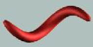
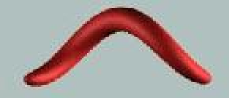
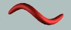
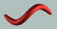
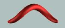
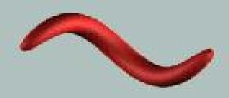
On the two figures below are given two theoretical examples with $\kappa=-1$ and $\kappa=1$ respectively, at a fixed moment $t$. For $t\in(-\infty,+\infty)$, the amplitude function $\phi$ fills in a smoothed out tube around a circular helix of height $2\pi\mathcal{L}_{o}$ and pitch $\mathcal{L}_{o}$, and phase function $\varphi=\mathrm{cos}(\kappa z/\mathcal{L}_{o})$. The solutions propagate left-to-right along the euclidean coordinate $z$.

Figure 1: Theoretical example with $\kappa=-1$. The Poynting vector is directed left-to-right.

Figure 2: Theoretical example with $\kappa=1$. The Poynting vector is directed left-to-right.

The integral of $\beta_{\mathbb{R}^{3}}$ over the 3-space for such solutions gives

$$\int_{\mathbb{R}^{3}}\beta_{\mathbb{R}^{3}}=\kappa E\frac{2\pi\mathcal{L}_{o}}{c}=\kappa ET=\pm ET,$$

where $E=\int_{\mathbb{R}^{3}}*(Q_{\mu 4}dx^{\mu})=\int_{\mathbb{R}^{3}}\phi^{2}d^{3}v$ is the integral energy of the solution, $T=2\pi\mathcal{L}_{o}/c$ is the intrinsically defined time-period, and $\kappa=\pm 1$ accounts for the two polarizations. Clearly, this integral may be interpreted as spin-momentum of the solution for one period $T$. Finally, the constant $\mathcal{L}_{o}$ may be intrinsically defined by

$$\mathcal{L}_{o}=\frac{|A|}{|\delta F|}=\frac{|A^{*}|}{|\delta*F|}.$$

7 Conclusion

Compare to the classical view, the basic difference of our approach to relativistically describe electromagnetic field objects consists mainly in the following steps: 1. These objects are considered as spatially finite and permanently propagating with the fundamental velocity ”c”, so their stress-energy-momentum tensor $Q_{\mu\nu}$ must be null : $Q_{\mu\nu}Q^{\mu\nu}=0$.

2. Every electromagnetic field object is a special kind of a physical object: it is built of two recognizable, time-stable and appropriately interacting subsystems, formally represented by the two differential 2-forms $(F,*F)$ on Minkowski space-time.

3. The null natuere of these objects: $Q_{\mu\nu}Q^{\mu\nu}=I_{1}^{2}+I_{2}^{2}=0$, requires the two subsystems to carry the same nonzero energy-momentum: $I_{1}=0\rightarrow F_{\mu\sigma}F^{\mu\sigma}=(*F)_{\mu\sigma}(*F)^{\mu\sigma}$, and to interact without interaction energy: $I_{2}=0\rightarrow F_{\mu\sigma}(*F)^{\mu\sigma}=0$.

4. The two subsystems admit recognizable nonzero changes, formally represented by $(\mathbf{d}F,\mathbf{d}*F)$.

5. The two subsystems live in a permanent dynamical equilibrium through realizing a local energy-momentum exchange according to the relations:

$$F^{\mu\nu}(\mathbf{d}F)_{\mu\nu\sigma}=0,\ \ (*F)^{\mu\nu}(\mathbf{d}*F)_{\mu\nu\sigma}=0,\ \ F^{\mu\nu}(\mathbf{d}*F)_{\mu\nu\sigma}=-(*F)^{\mu\nu}\mathbf{d}F_{\mu\nu\sigma},\ \ \mu<\nu.$$

6. The equations, describing the corresponding intrinsic dynamics and space-time propagation as a whole of an electromagnetic field object through their nonlinear solutions, represent the understanding that the $\mathbb{R}^{2}$-valued 2-vector $\bar{\Omega}=\bar{F}\otimes e_{1}+\bar{*F}\otimes e_{2}$ is $(\mathbf{d},\vee)$ - algebraic and differential symmetry of the $\mathbb{R}^{2}$-valued 2-form $\Omega=F\otimes e_{1}+*F\otimes e_{2}$ according to the equations $i^{\vee}_{\bar{\Omega}}\Omega=\mathfrak{C}=0,\ \mathcal{L}^{\vee}_{\bar{\Omega}}\Omega=0$.

7. The space-time propagation of an electromagnetic field object has a compatible translational-rotational nature, and is characterized by a proportional to the object’s integral energy spin momentum, locally represented by the $F\leftrightarrow*F$ nonzero local energy-momentum exchange.

8. Formally, the existence of non-zero spin momentum is measured by the Frobenius non-integrability of the two geometric distributions defined by $\bar{F}=\bar{\zeta}\wedge\bar{A}$ and $\bar{*F}=\bar{\zeta}\wedge\bar{A}^{*}$. The last (No.8) step we consider as very suggestive in the following sense. When a continuous physical system consists of several recognizable interacting time-stable subsystems, and these subsystems admit natural representation as a number of geometric distributions and corresponding codistributions, then the Frobenius integrability relations to be essentially used as local measures of time stability of the subsystems, and the available curvature forms to be essentially used as local energy-momentum exchange ”communicators” among the subsytems. Also, if the whole system admits formal representation as geometric distribution, in order it to be time-stable, an external local time-like, or isotropic, symmetry must exist.

References

[1]. Stoil Donev, Maria Tashkova, A nonlinear prerelativistic approach to mathematical representation of vacuum electromagnetism, arXiv: hep-th/1303.2808v2

[2]. H. Lorentz, Electromagnetic phenomena in a system moving with any velocity smaller than that of light, Proc. Acad. Sci., Amsterdam, 1904, 6, (809); 12 (986)

[3]. A. Poincare, Sur la dynamique de l’electron, Comptes Rendue 1905, 140 (1504); Rendiconti dei Circole Matematico di Palermo, 1906, XXI (129)

[4]. A. Einstein, Zur Elektrodynamik bewegter Korper, Ann. d. Phys. 1905, 17 (891)

[5]. H. Minkowski, The Fundamental Equations for Electromagnetic Processes in Moving Bodies, lecture given at the meeting of the Gottingen Scientific Society, December 21, 1907; english vrsion at: http://www.minkowskiinstitute.org/mip/books/minkowski.html

[6]. G. Rainich, Electrodynamics in general Relativity, Trans.Amer.Math.Soc., 27 (106-136)

[7]. W. Misner, J. Wheeler, Classical Physics as geometry, Ann.Phys., 2 (525-603)

[8]. J. Franca, J. Lopez-Bonilla, The Algebraic Rainich Conditions, Progress in Physics, vol.3, July 2007

[9]. J.L.Synge, Relativity: The Special Theory, North-Holland, 1956, Ch.IX, § 7.

[10]. P. Michor, Topics in Differential Geometry, AMS, 2008

[11]. W. Greub, Multilinear Algebra, first edition, Springer-Verlag, 1967

[12]. M. Forger, C. Paufler, H. Reomer, The Poisson Bracket for Poisson Forms in Multisymplectic Field Theory, arXiv: math-ph/0202043v1

[13]. C. Godbillon, Geometrie differentielle et mecanique analytiqe, Hermann, Paris (1969)

[14]. A. Kushner, V. Lychagin, V. Rubtsov,, Contact Geometry and Non-linear Differential Equations, Cambridge University Press 2007

[15]. Donev, S., Tashkova, M., Geometric View on Photon-like Objects, arXiv: math-ph/1210.8323 (published as monograph by LAP-Publishing)