Full-sky formulae for weak lensing power spectra from total angular momentum method

Abstract

We systematically derive full-sky formulae for the weak lensing power spectra generated by scalar, vector and tensor perturbations from the total angular momentum (TAM) method. Based on both the geodesic and geodesic deviation equations, we first give the gauge-invariant expressions for the deflection angle and Jacobi map as observables of the CMB lensing and cosmic shear experiments. We then apply the TAM method, originally developed in the theoretical studies of CMB, to a systematic derivation of the angular power spectra. The TAM representation, which characterizes the total angular dependence of the spatial modes projected along a line-of-sight, can carry all the information of the lensing modes generated by scalar, vector, and tensor metric perturbations. This greatly simplifies the calculation, and we present a complete set of the full-sky formulae for angular power spectra in both the E-/B-mode cosmic shear and gradient-/curl-mode lensing potential of deflection angle. Based on the formulae, we give illustrative examples of non-vanishing B-mode cosmic shear and curl-mode of deflection angle in the presence of the vector and tensor perturbations, and explicitly compute the power spectra.

1 Introduction

Precision weak lensing measurement in cosmology is the key to improve our view of the Universe, and it directly offers an opportunity to probe unseen cosmological fluctuations along a line-of-sight of photon path. In particular, planned wide- and deep-imaging surveys such as Subaru Hyper Supreme-Can (HSC) [1], Dark Energy Survey (DES) [2], Euclid [3], and Large Synaptic Survey Telescope (LSST) [4] will provide a high-precision measurement of the deformation of the distant-galaxy images, whose non-vanishing spatial correlation is primarily caused by the gravitational lensing. The so-called cosmic shear is now recognized as a standard cosmological tool, and plays an important role to constrain the growth of structure and/or cosmic expansion [5, 6, 7, 8, 9, 10, 11, 12, 13, 14, 15] (for reviews, see [16, 17, 18, 19]). On the other hand, cosmic microwave background also carries the information on the gravitational lensing, and through the sophisticated reconstruction techniques, one can measure the gravitational lensing deflection of the CMB photons, referred to as the CMB-lensing signals. The ground-based experiments, Atacama Cosmology Telescope (ACT) [20, 21] and South Pole Telescope (SPT) [22], as well as Planck satellite have already revealed the undoubted lensing signals [23], and future CMB experiments, including, POLARBEAR [24], ACTPol [25], SPTPol [26], CMBPol [27], and COrE [28], will measure the lensing deflection field much more precisely.

While the weak lensing effect detected and measured so far is mostly dominated by the scalar metric perturbation induced by the large-scale structure, with an increased precision, a search for tiny signals generated by the vector and tensor perturbations is made possible, and the detection and/or measurement of such signals would provide a valuable insight into the physics and history of the very early universe. Theoretically, the distortion effect of lensing on the primary CMB anisotropies is expressed by a remapping with two dimensional vector, usually referred to as deflection angle, which can be estimated through the fact that a fixed lensing potential introduces statistical anisotropy into the observed CMB. Hence we consider the CMB lensing as being a solution of geodesic equation. On the other hand, for galaxy survey, what we can measure is the shape (or shear) of galaxies modified by gravitational lensing, which is characterized by the deformation of two-dimensional spatial pattern. Therefore we solve the geodesic deviation equation for the shear field. The lensing fields can be generally decomposed into two modes: the gradient of scalar lensing potential (gradient-mode) and rotation of pseudo-scalar lensing potential (curl-mode) for deflection angle (e.g., [14, 29, 30]), and the even- and odd-parity modes (E-/B-modes) for cosmic shear (e.g., [14, 15]). One important aspect from the symmetric argument is that the scalar perturbation can produce both the E-mode shear and the gradient-mode lensing potential of the deflection angle, while it is unable to generate the B-mode shear and the curl-mode lensing potential. Hence, non-vanishing B-mode or curl-mode signal on large angular scales immediately implies the presence of non-scalar metric perturbations.

In this paper, we systematically derive the angular power spectra of gradient-/curl-mode lensing potential and E-/B-mode cosmic shear, and present a complete set of full-sky formula for scalar, vector, and tensor metric perturbations. As illustrative examples, we consider the cosmic strings and primordial gravitational waves as representative sources for vector and tensor perturbations. Based on the formulae, we explicitly compute the power spectra, showing that the non-vanishing B-mode and curl-mode lensing signals naturally arise. In deriving the weak lensing power spectra, one complication is that while the weak lensing observables are defined on a spherical sky, the metric perturbations as the source of the gravitational lensing usually appear in the three-dimensional space. Thus, even decomposing the perturbations into the plane waves, due to their angular structure, a plane wave along a line-of-sight can contribute to the lensing observables at several multipoles. The situation is more complicated for the vector and tensor perturbations, since the helicity basis of their perturbations also has explicit angular dependence, and contributes to many multipoles. One way to avoid these complications is to isolate the total angular dependence of the perturbations by introducing new representation, the total angular momentum (TAM) representation [31] (see also [32]), originally developed in the theoretical studies of CMB. Combining the intrinsic angular structure with that of the plane-wave spatial dependence, the total angular momentum representation substantially simplifies the derivation of the full-sky formula, and it enables us to simultaneously treat the weak lensing by vector and tensor perturbations on an equal footing with those generated by scalar perturbation. As a result, we obtain a complete set of power spectra in both the cosmic shear and lensing potential of deflection angle. Our full-sky formulae rigorously coincide with those obtained previously based on a more involved calculation (see [36, 33, 35, 37, 38, 34, 39] for vector and tensor perturbations).

The paper is organized as follows. We begin by defining the unperturbed and perturbed spacetime metrics, and quantities associated with the photon path in section 2. In section 3, based on the gauge-invariant formalism, we solve the geodesic and geodesic deviation equations in the presence of all types of the metric perturbations. We then derive the explicit relation between the deflection angle and the deformation matrix. Section 4 is the main part of this paper. We introduce the TAM representation, and rewrite the expression of the lensing observables in term of this representation. Making full use of the properties of the TAM representation, we present the full-sky formulae for angular power spectra of the E-/B-mode cosmic shear and the gradient-/curl-mode lensing potential. In section 5, based on the formulae, we give illustrative examples of non-vanishing B-mode and curl-mode lensing signals in the presence of the vector and tensor perturbations, and explicitly compute the power spectra. Finally, section 6 is devoted to summary and conclusion. Throughout the paper, we assume a flat $\Lambda$CDM cosmological model with the cosmological parameters : $\Omega_{\rm b}h^{2}=0.22$ , $\Omega_{\mathrm{m}}h^{2}=0.13$ , $\Omega_{\Lambda}=0.72$ , $h=0.7$ , $n_{\rm s}=0.96$ , $\Delta_{\mathcal{R}}^{2}(k_{\rm pivot})=2.4\times 10^{-9}$ , $k_{\rm pivot}=0.002{\rm Mpc}^{-1}$ , $r=0.2$ , $n_{\rm t}=-r/8=-0.025$ , $\tau=0.086$ . In Table 1, we list the definition of the quantities used in the paper.

Table 1: Notations for quantities used in this paper.

Symbol	eq.	Definition
$g_{\mu\nu}$	(2.2)	$4$-dimensional metric on unperturbed spacetime
$\bar{\gamma}_{ij}$	(2.2)	$3$-dimensional spatial metric
$\omega_{ab}$,$\epsilon_{ab}$	-	Metric/Levi-Civita pseudo-tensor on unit sphere
vertical bar ( $|$ )	-	Covariant derivative associated with $\bar{\gamma}_{ij}$
colon ( $:$ )	(A.32)	Covariant derivative associated with $\omega_{ab}$
$\chi$	-	Affine parameter on unperturbed spacetime
$\mathrm{d}x^{\mu}/\mathrm{d}\chi$	(2.10)	Wave vector on unperturbed spacetime
$\hat{\bm{n}}$	-	line-of-sight vector
${\bm{e}}_{a},{\bm{e}}_{\pm}$	(2.12)	Basis of spin-weight $\pm 1$
$\Phi,\Psi$	(2.6)	Gauge-invariant scalar metric perturbations
$\sigma_{\mathrm{g},i}$	(2.7)	Gauge-invariant vector metric perturbations
$h_{ij}$	(2.5)	Tensor metric perturbations
$\Upsilon$	(3.6)	Spin-$0$ gauge-invariant combination
$\Omega_{a}$	(3.8)	Spin-$\pm 1$ gauge-invariant combination
$\Psi_{\bm{k}}^{(m)}$	(4.50)	Fourier coefficients for mode-$m$ gauge-invariant perturbations
$\Delta^{a}$	(3.10)	Deflection angle on unit sphere
$\phi,\varpi$	(3.11)	Scalar/pseudo-scalar lensing potentials
$\mathcal{D}^{a}{}_{b}$	(3.15)	Jacobi map
$\mathcal{T}^{a}{}_{b}$	(3.16)	Symmetric optical tidal matrix
$\gamma_{ab}$	(3.19)	shear field
$E,B$	(4.66)	E-/B-mode reduced cosmic shear
${}_{s}G_{\ell}{}^{m}$	(4.1)	basis function
${}_{s}\epsilon_{L}^{(\ell,m)},{}_{s}\beta_{L}^{(\ell,m)}$	(4.4)	Radial E,B function
$Q^{(0)},Q^{(\pm 1)}_{i},Q^{(\pm 2)}_{ij}$	(4.6),(4.9),(4.13)	spin-$0$,$\pm 1$,$\pm 2$ basis
$\ooalign{\hfil/\hfil\crcr$\partial$},\bar{\ooalign{\hfil/\hfil\crcr$\partial$}}$	(A.6),(A.9)	spin-raising/lowering operators
$\mathcal{S}_{x,\ell}^{(m)}$	(4.51)-(4.56)	Transfer function for gradient-/curl-modes
$\mathcal{S}_{\mathrm{X},\ell}^{(m)}$	(4.84)-(4.89)	Transfer function for E-/B-modes
$\mathcal{M}_{\ell}^{\mathrm{X}\mathrm{X}}{}^{(m)}$	(4.59),(4.91)	Auto-power spectrum for $X_{\ell}{}^{(m)}({\bm{k}})$
$C_{\ell}^{\mathrm{X}\mathrm{X}}$	(4.18),(4.67)	Angular power spectrum for $X_{\ell m}$
$\mathcal{P}_{|m|}$	(4.57)	Auto-power spectrum for $\Psi_{\bm{k}}^{(m)}$

2 Background and perturbations

In this paper, we consider the flat FLRW universe with the metric given by

$$\mathrm{d}s^{2}=a^{2}(\eta)\tilde{g}_{\mu\nu}\mathrm{d}x^{\mu}\mathrm{d}x^{\nu}= a^{2}(\eta)\bigl{(}g_{\mu\nu}+\delta g_{\mu\nu}\bigr{)}\mathrm{d}x^{\mu}\mathrm{d}x^{\nu}\,,$$ (2.1)

where $a(\eta)$ corresponds to the conventional scale factor of a homogeneous and isotropic universe, $\tilde{g}_{\mu\nu}$ is the conformal flat four-dimensional metric which includes the spacetime inhomogeneity, $\delta g_{\mu\nu}$ is small metric perturbations. Here, $g_{\mu\nu}$ is the conformally related metric assumed to have the following form:

$$g_{\mu\nu}\mathrm{d}x^{\mu}\mathrm{d}x^{\nu}=-\mathrm{d}\eta^{2}+\bar{\gamma}_{ij}\mathrm{d}x^{i}\mathrm{d}x^{j}=-\mathrm{d}\eta^{2}+\mathrm{d}\chi^{2}+\chi^{2}\omega_{ab}\mathrm{d}\theta^{a}\mathrm{d}\theta^{b}\,,$$ (2.2)

where $\omega_{ab}=\mathrm{d}\theta^{2}+\sin^{2}\theta\mathrm{d}\varphi^{2}$ is the metric on the unit sphere. In what follows, tensors defined on the perturbed spacetime will be distinguished by the indication of a tilde ( $\tilde{}$ ) as above. The small departure of the metric from the background metric $g_{\mu\nu}$ can be represented as a set of metric perturbations:

$$\delta g_{00}=-2A\,,$$ (2.3)

$$\delta g_{0i}=B_{|i}+B_{i}\,,$$ (2.4)

$$\delta g_{ij}=2\mathcal{R}\bar{\gamma}_{ij}+2H_{|ij}+H_{i|j}+H_{j|i}+h_{ij}\,,$$ (2.5)

where $B_{i}$ and $H_{i}$ are divergence-free three-vectors, $h_{ij}$ is the transverse-traceless tensor, and the vertical bar ( $|$ ) denotes the covariant derivative with respect to the three-dimensional metric $\bar{\gamma}_{ij}$ .

Based on the gauge transformation properties, independent gauge-invariant quantities can be constructed from these variables. One possible choice of such invariants are [40]

$$\Phi\equiv A-\frac{1}{a}\left(a\left(\dot{H}-B\right)\right)^{\cdot}\,,\ \ \ \Psi\equiv\mathcal{R}-\frac{\dot{a}}{a}\left(\dot{H}-B\right)\,,$$ (2.6)

where the dot ( $\dot{}$ ) denotes the derivative with respect to the conformal time $\eta$ . These combinations corresponds to the Bardeen’s invariants and they are chosen as the appropriate variables for the conformal Newton-gauge. We also have the gauge-invariant vector metric perturbations: [40]

$$\sigma_{\mathrm{g},i}\equiv\dot{H}_{i}-B_{i}\,.$$ (2.7)

For tensor perturbations, there exists no tensor-type infinitesimal gauge transformation. Hence all the quantities associated with tensor perturbations are gauge-invariant by themselves. Appendix B summarizes the Christoffel symbols and Riemann tensors from the metric perturbations $\delta g_{\mu\nu}$ .

Figure 1: Representation of the direction vector $\hat{\bm{n}}$ , and the two orthogonal vectors along the light ray $\{{\bm{e}}_{\theta}\,,{\bm{e}}_{\phi}\}$ . At the observer position, these vectors form a basis, which can be parallel transported along the geodesic.

We consider two null geodesics on the physical spacetime : $x^{\mu}(v)$ and $\tilde{x}^{\mu}(v)=x^{\mu}(v)+\xi^{\mu}(v)$ , where $v$ is the affine parameter along the photon path and $x^{\mu}(v)$ and $\xi^{\mu}(v)$ are a reference geodesic and a deviation vector labeling the reference geodesic. It is known that the conformal transformation $a^{2}g_{\mu\nu}\rightarrow g_{\mu\nu}$ maps a null geodesic on the physical spacetime to a null geodesic on the conformally transformed spacetime with the affine parameter transformed as $\mathrm{d}v\rightarrow\mathrm{d}\lambda=a^{-2}\mathrm{d}v$ [41, 11] . In the cosmological background, it is sufficient to perform the calculation without the Hubble expansion and reintroduce the scale factor at the end by scaling $\mathrm{d}\lambda\rightarrow\mathrm{d}v=a^{2}\mathrm{d}\lambda$ . Hence, we define a tangent vector $k^{\mu}$ on the conformally transformed spacetime as

$$k^{\mu}\equiv a^{2}\frac{\mathrm{d}x^{\mu}}{\mathrm{d}v}=\frac{\mathrm{d}x^{\mu}}{\mathrm{d}\lambda}\,.$$ (2.8)

This is a null vector satisfying the equations:

$$g_{\mu\nu}k^{\mu}k^{\nu}=0\,,\ \ \ \frac{\mathrm{D}k^{\mu}}{\mathrm{d}\lambda}\equiv\frac{\mathrm{d}^{2}x^{\mu}}{\mathrm{d}\lambda^{2}}+\Gamma^{\mu}_{\rho\sigma}\frac{\mathrm{d}x^{\rho}}{\mathrm{d}\lambda}\frac{\mathrm{d}x^{\sigma}}{\mathrm{d}\lambda}=0\,,$$ (2.9)

where $\Gamma^{\mu}_{\rho\sigma}$ is the Christoffel symbols associated with the metric on the unperturbed universe, $g_{\mu\nu}$ . We can solve the above geodesic equation to obtain $x^{\mu}(\lambda)=E(\lambda,(\lambda_{0}-\lambda)\hat{\bm{n}})$ , where $E$ and $\hat{\bm{n}}$ represent the photon energy and the propagation direction measured from the observer in the background flat spacetime , $\lambda_{0}$ denotes the affine parameter at the observer. $\hat{\bm{n}}$ is the unit vector tangent to geodesic on the flat three-space, satisfying $\hat{\bm{n}}\cdot\hat{\bm{n}}=1$ and $\hat{n}^{i}{}_{|j}\hat{n}^{j}=0$ . Here we have switched from $\lambda$ to $\chi\equiv E(\lambda_{0}-\lambda)$ . We then have the wave vector in the unperturbed universe:

$$\frac{\mathrm{d}x^{\mu}}{\mathrm{d}\chi}=\left(-1\,,\,\hat{\bm{n}}\right)\,.$$ (2.10)

We also denote by $u^{\mu}$ the background observer’s four-velocity at the observer’s position, with the normalization condition $g_{\mu\nu}u^{\mu}u^{\nu}=-1$ . With these notations, we define orthogonal spacetime basis along the light ray, $e^{\mu}_{a}$ with $a=\theta\,,\varphi$ , which obey

$$g_{\mu\nu}e^{\mu}_{a}e^{\nu}_{b}=\omega_{ab}\,,\ \ g_{\mu\nu}k^{\mu}e^{\nu}_{a}=g_{\mu\nu}u^{\mu}e^{\nu}_{a}=0\,.$$ (2.11)

They are parallel transported along the geodesics : $(\mathrm{D}/\mathrm{d}\chi)u^{\mu}=0$ , $(\mathrm{D}/\mathrm{d}\chi)e^{\mu}_{a}=0$ . Representation of light bundle, the deviation vector, and the basis vectors is shown in fig. 1. Considering a static observer, $u^{\mu}=(1,{\bm{0}})$ , the basis vector $e^{\mu}_{a}$ can be described as $e^{\mu}_{a}=(0,{\bm{e}}_{a})$ . To discuss the spatial pattern on celestial sphere, it is useful to introduce the spin-weighted quantities. The polarization vector with respect to a two-dimensional vector on the sky is expected in terms of two vector basis ${\bm{e}}_{\theta}(\hat{\bm{n}})$ and ${\bm{e}}_{\varphi}(\hat{\bm{n}})$ perpendicular to the line-of-sight vector ${\bm{n}}$ as [42]

$${\bm{e}}_{\pm}(\hat{\bm{n}})={\bm{e}}_{\theta}(\hat{\bm{n}})\pm\frac{i}{\sin\theta}\,{\bm{e}}_{\varphi}(\hat{\bm{n}})\,.$$ (2.12)

We list the explicit expression for the basis vectors, $\hat{\bm{n}}$ and ${\bm{e}_{a}}$ , in the Cartesian coordinates in Appendix A.3.

3 Weak lensing observables

In this section, we consider the deformation of the cross-section of a congruence of null geodesics under propagation in a perturbed universe. We give the basic equations which govern the weak gravitational lensing effect in the presence of scalar, vector and tensor metric perturbations by solving the geodesic equation in section 3.1 and the geodesic deviation equation in section 3.2. Based on the results, we derive an explicit relation between the gradient of the deflection angle and the Jacobi matrix.

3.1 Deflection angle

In order to see the lensing effect, let us consider the spatial components of the geodesic equation for the photon ray. To derive the first-order geodesic equation, we parametrize the perturbed photon geodesic as

$$\frac{\mathrm{d}\tilde{x}^{\mu}}{\mathrm{d}\chi}=\left(-1+\delta\nu\,,\,\hat{\bm{n}}+\delta{\bm{e}}\right)\,.$$ (3.1)

Based on the gauge transformation properties, we can construct the gauge-invariant components of perturbed wave vector [43]:

$$\delta\nu_{\rm GI}=\delta\nu+2\frac{\dot{a}}{a}\sigma_{\mathrm{g}}^{(\mathrm{S})}-\frac{\mathrm{d}}{\mathrm{d}\chi}\sigma_{\mathrm{g}}^{(\mathrm{S})}\,,$$ (3.2)

$$\delta e_{\rm GI}^{i}=\delta e^{i}+2\frac{\dot{a}}{a}\sigma_{\mathrm{g}}^{(\mathrm{S})}\hat{n}^{i}+\frac{\mathrm{D}}{\mathrm{d}\chi}\mathcal{G}^{i}-\mathcal{G}^{j}\hat{n}^{i}{}_{|j}\,,$$ (3.3)

where $\sigma_{\mathrm{g}}^{(\mathrm{S})}\equiv\dot{H}-B$ and $\mathcal{G}_{i}\equiv(H_{|i}+H_{i})$ are the pure gauge terms. They are chosen as the appropriate variables for the conformal Newton gauge. To derive the first-order geodesic equation, we expand the Christoffel symbols as $\tilde{\Gamma}^{\mu}_{\rho\sigma}=\Gamma^{\mu}_{\rho\sigma}+\delta\Gamma^{\mu}_{\rho\sigma}$ , where $\tilde{\Gamma}^{\mu}_{\rho\sigma}$ is the Christoffel symbols associated with the metric on the perturbed universe, $\tilde{g}_{\mu\nu}$ (see Appendix B) . In the conformally transformed spacetime, we then derive the null condition, the temporal and spatial components of the geodesic equation in terms of the gauge-invariant quantities:

$$\hat{\bm{n}}\cdot\delta{\bm{e}}_{\rm GI}=\delta\nu_{\rm GI}-\Upsilon\,,\ \ \ \ \frac{\mathrm{d}}{\mathrm{d}\chi}\Bigl{(}\delta\nu_{\rm GI}+2\Phi-\sigma_{\mathrm{g},i}\hat{n}^{i}\Bigr{)}=\dot{\Upsilon}\,,$$ (3.4)

$$\frac{\mathrm{D}}{\mathrm{d}\chi}\Bigl{(}\delta e^{i}_{\rm GI}+2\Psi\hat{n}^{i}+\sigma_{\mathrm{g}}{}^{i}+h^{i}{}_{j}\hat{n}^{j}\Bigr{)}=-\delta e^{j}_{\rm GI}\,\hat{n}^{i}{}_{|j}+\left(\Psi-\Phi\right)^{|i}+\sigma_{\mathrm{g}\,j}{}^{|i}\hat{n}^{j}+\frac{1}{2}h_{jk}{}^{|i}\hat{n}^{j}\hat{n}^{k}\,,$$ (3.5)

where $(\mathrm{D}/\mathrm{d}\chi)\zeta^{i}\equiv\hat{n}^{j}\zeta^{i}{}_{|j}-\partial_{\eta}\zeta^{i}$ and we have introduced the gauge-invariant combination of the spin-$0$ components constructed from the scalar, vector, and tensor perturbations as

$$\Upsilon\equiv\Psi-\Phi+\sigma_{\mathrm{g},i}\,\hat{n}^{i}+\frac{1}{2}\,h_{ij}\,\hat{n}^{i}\hat{n}^{j}\,.$$ (3.6)

The equations we have derived here are manifestly gauge-invariant because the gauge degrees of freedoms in the explicit expressions for the geodesic equation are completely canceled.

In addition to the wave vector, we introduce the gauge-invariant deviation vector as $\delta e^{i}_{\rm GI}\equiv(\mathrm{d}/\mathrm{d}\chi)\xi^{i}_{\rm GI}$ . To extract the angular components of the deviation vector, $\xi^{a}_{\rm GI}\equiv\xi^{i}_{\rm GI}e_{i}^{a}$, we multiply $e_{i}^{a}$ in both side of eq. (3.5) . Since the unperturbed Christoffel symbols satisfies $\Gamma^{i}_{jk}=0$ in the Cartesian coordinate system, with the condition for the parallel transformation, $(\mathrm{D}/\mathrm{d}\chi)e_{i}^{a}=0$ , we obtain

$$\frac{\mathrm{d}^{2}\xi^{a}_{\rm GI}}{\mathrm{d}\chi^{2}}=\frac{1}{\chi}\omega^{ab}\biggl{\{}\Upsilon_{:b}-\frac{\mathrm{d}}{\mathrm{d}\chi}\bigl{(}\chi\Omega_{b}\bigr{)}\biggr{\}}\,.$$ (3.7)

where we have introduced the gauge-invariant combination of the spin-$\pm 1$ components constructed from the vector and tensor metric perturbations:

$$\Omega_{a}\equiv\left(\sigma_{\mathrm{g},j}+h_{ij}\hat{n}^{i}\right)e^{j}_{a}\,.$$ (3.8)

Given the initial conditions, $\xi^{a}_{\rm GI}|_{0}=0$ , and $(\mathrm{d}\xi^{a}_{\rm GI}/\mathrm{d}\chi)|_{0}=\delta\theta_{0}^{a}$ , where $\delta\theta^{a}_{0}$ denotes the angular coordinate at the observer position, the deviation vector as

$$\frac{\xi^{a}_{\rm GI}}{\chi_{\rm S}}= \,\delta\theta^{a}_{0}+\omega^{ab}\int^{\chi_{\rm S}}_{0}\mathrm{d}\chi\frac{\chi_{\rm S}-\chi}{\chi_{\rm S}\chi}\biggl{\{}\Upsilon_{:b}-\frac{\mathrm{d}}{\mathrm{d}\chi}\bigl{(}\chi\Omega_{b}\bigr{)}\biggr{\}}\biggl{|}_{(\eta_{0}-\chi,\chi\hat{\bm{n}})}\,.$$ (3.9)

The integration at the right-hand-side is evaluated along the unperturbed light path $x^{\mu}(\chi)=(\eta_{0}-\chi,\chi\hat{\bm{n}})$ , where $\eta_{0}$ denotes the conformal time at the observer, according to the Born approximation. For simplicity, we omit the subscript $(\eta_{0}-\chi,\chi\hat{\bm{n}})$ hereafter. Given the angular direction at both end points, the deflection angle, $\Delta^{a}$, can be estimated through [14]

$$\Delta^{a}\equiv\frac{\xi^{a}_{\rm GI}}{\chi_{\rm S}}-\delta\theta^{a}_{0}\,.$$ (3.10)

Since the deflection angle is the two-dimensional vector field defined on the celestial sphere, it is generally characterized by the sum of two potentials; a gradient of scalar lensing potential ($\phi$) (gradient-mode), and a rotation of pseudo-scalar lensing potential ($\varpi$) (curl-mode) [29]:

$$\Delta^{a}=\phi_{:a}+\varpi_{:b}\epsilon^{b}{}_{a}\,.$$ (3.11)

where $\epsilon^{b}{}_{a}$ denotes the two-dimensional Levi-Civita pseudo-tensor. Integrating by part, the gradient-/curl-mode lensing potentials can be written as

$$\phi^{:a}{}_{:a}=\Delta^{a}{}_{:a}=\int^{\chi_{\rm S}}_{0}\mathrm{d}\chi\frac{\chi_{\rm S}-\chi}{\chi_{\rm S}\chi}\biggl{\{}\Upsilon^{:a}{}_{:a}-\frac{\mathrm{d}}{\mathrm{d}\chi}\left(\chi\Omega^{a}{}_{:a}\right)\biggr{\}}\,,$$ (3.12)

$$\varpi^{:a}{}_{:a}=\Delta^{a}{}_{:b}\epsilon^{b}{}_{a}=-\int^{\chi_{\rm S}}_{0}\mathrm{d}\chi\frac{\chi_{\rm S}-\chi}{\chi_{\rm S}\chi}\frac{\mathrm{d}}{\mathrm{d}\chi}\left(\chi\Omega^{a}{}_{:b}\epsilon^{b}{}_{a}\right)\,.$$ (3.13)

3.2 Jacobi map

Let us consider the Jacobi map which characterizes the deformation of light bundle. In terms of the projected deviation vector $\xi^{a}$ , the geodesic deviation equation in the conformally transformed spacetime can be written as [8, 12]

$$\frac{\mathrm{d}^{2}\xi^{a}}{\mathrm{d}\chi^{2}}=\tilde{\mathcal{T}}^{a}{}_{b}\,\xi^{b}\,;\ \ \tilde{\mathcal{T}}^{a}{}_{b}=-\tilde{R}_{\mu\rho\nu\sigma}\frac{\mathrm{d}x^{\mu}}{\mathrm{d}\chi}\frac{\mathrm{d}x^{\nu}}{\mathrm{d}\chi}e^{\rho a}e^{\sigma}_{b}\,,$$ (3.14)

where $\tilde{\mathcal{T}}^{a}{}_{b}$ is the symmetric optical tidal matrix, and $\tilde{R}_{\mu\rho\nu\sigma}$ is the Riemann tensor associated with the metric $\tilde{g}_{\mu\nu}$ . Provided the initial conditions at the observer, $\xi^{a}|_{0}=0$ and $(\mathrm{d}\xi^{a}/\mathrm{d}\chi)|_{0}=\delta\theta_{0}^{a}$ , the solution of eq. (3.14) can be written in terms of the Jacobi map as

$$\xi^{a}=\tilde{\mathcal{D}}^{a}{}_{b}\,\delta\theta^{b}_{0}\,,$$ (3.15)

where the Jacobi map $\tilde{\mathcal{D}}^{a}{}_{b}$ satisfies

$$\frac{\mathrm{d}^{2}}{\mathrm{d}\chi^{2}}\tilde{\mathcal{D}}^{a}{}_{b}=\tilde{\mathcal{T}}^{a}{}_{c}\tilde{\mathcal{D}}^{c}{}_{b}\,,$$ (3.16)

with the initial condition for the Jacobi map : $\tilde{\mathcal{D}}^{a}{}_{b}|_{0}=0$ and $(\mathrm{d}/\mathrm{d}\chi)\tilde{\mathcal{D}}^{a}{}_{b}|_{0}=\delta^{a}{}_{b}$ .

To obtain the expression relevant for the weak lensing measurements, we expand as $\tilde{\mathcal{D}}^{a}{}_{b}=\mathcal{D}^{a}{}_{b}+\delta\mathcal{D}^{a}{}_{b}$ and $\tilde{\mathcal{T}}^{a}{}_{b}=\mathcal{T}^{a}{}_{b}+\delta\mathcal{T}^{a}{}_{b}$ . Since $\mathcal{T}^{a}{}_{b}=0$ in unperturbed spacetime, the zeroth-order solution of Jacobi map trivially reduces to $\mathcal{D}^{a}{}_{b}=\chi\delta^{a}{}_{b}$ . Substituting this expression into eq. (3.16) and solving this equation, we have the Jacobi map up to linear order:

$$\frac{1}{\chi_{\rm S}}\tilde{\mathcal{D}}^{a}{}_{b}=\delta^{a}{}_{b}+\int^{\chi_{\rm S}}_{0}\mathrm{d}\chi\frac{\left(\chi_{\rm S}-\chi\right)\chi}{\chi_{\rm S}}\,\delta\mathcal{T}^{a}{}_{b}(\eta_{0}-\chi,\chi\hat{\bm{n}})+\mathcal{O}(\delta g_{\mu\nu}^{2})\,.$$ (3.17)

We are now interested in the shear fields, namely the symmetric trace-free part of the Jacobi map. We introduce the bracket $\left\langle\cdots\right\rangle$ , which denotes the symmetric trace-free part taken in the two-dimensional space: $X_{\left\langle ab\right\rangle}=(1/2)(X_{ab}+X_{ba}-X^{c}{}_{c}\,\omega_{ab})$ . To derive the expression relevant for the arbitrary metric perturbations eq. (2.1), we explicitly write down the symmetric trace-free part of the linear-order symmetric optical tidal matrix as (see Appendix B)

$$\chi^{2}\,\delta\mathcal{T}_{\left\langle ab\right\rangle}=\Upsilon_{\left\langle:ab\right\rangle}-\frac{\mathrm{d}}{\mathrm{d}\chi}\Bigl{(}\chi\Omega_{\left\langle a:b\right\rangle}\Bigr{)}+\frac{1}{2}\chi\frac{\mathrm{d}^{2}}{\mathrm{d}\chi^{2}}\left(\chi h_{\left\langle ab\right\rangle}\right)\,,$$ (3.18)

where $\Upsilon$ and $\Omega_{a}$ were defined in eqs. (3.6) and (3.8) , we have defined $h_{ab}=h_{ij}e^{i}_{a}e^{j}_{b}$ . Substituting eq. (3.18) into eq. (3.17) and integrating by part, we obtain the explicit expression for the first-order cosmic shear as

$$\gamma_{ab}\equiv \frac{1}{\chi_{\rm S}}\tilde{\mathcal{D}}_{\left\langle ab\right\rangle}=\int^{\chi_{\rm S}}_{0}\mathrm{d}\chi\frac{\chi_{\rm S}-\chi}{\chi_{\rm S}\chi}\biggl{\{}\Upsilon_{:\left\langle ab\right\rangle}-\frac{\mathrm{d}}{\mathrm{d}\chi}\left(\chi\Omega_{\left\langle a:b\right\rangle}\right)\biggr{\}}+\frac{1}{2}\bigl{[}h_{\left\langle ab\right\rangle}\bigr{]}^{\chi_{\rm S}}_{0}\,,$$ (3.19)

where $[\zeta]^{\chi_{1}}_{\chi_{2}}\equiv\zeta(\eta_{0}-\chi_{1},\chi_{1}\hat{\bm{n}})-\zeta(\eta_{0}-\chi_{2},\chi_{2}\hat{\bm{n}})$ . Since the gauge degrees of freedom are completely removed in the explicit expression for the symmetric optical tidal matrix (3.18), the resulting shear field we have derived here are manifestly gauge-invariant.

Finally, comparing between (3.9), (3.11), and (3.19) , we find the explicit relation between the deflection angle and the deformation matrix:

$$\gamma_{ab}= \Delta_{\left\langle a:b\right\rangle}+\frac{1}{2}\bigl{[}h_{\left\langle ab\right\rangle}\bigr{]}^{\chi_{\rm S}}_{0}\,.$$ (3.20)

This relation is one of the main results in this paper. Although cosmic shear measurement via galaxy survey are usually referenced to the coordinate in which galaxies are statistically isotropic, this is in general different from our reference coordinate, namely flat FLRW universe. Hence, the correction from the gravitational potential at the source should appear in the observed shear field. Such correction corresponds to the last term at the right-hand-side in eq. (3.20) and is referred to as the metric shear/Fermi Normal Coordinate (FNC) term, which has been discussed in Refs. [33, 35, 34]. In contrast to the previous studies based on the geodesic equation, the metric shear/FNC term naturally arises in our case from the geodesic deviation equation. This is understood as follow: Since the leading correction of the metric in the FNC is known to be described by the Riemann curvature, it contains the information of the difference between the FNC and the flat FLRW coordinates. Therefore the FNC contribution is automatically included in the symmetric tidal matrix perturbed around the flat FLRW universe. Furthermore the geodesic equation contains only up to the first line-of-sight derivative on the metric perturbations, while the metric shear/FNC term is a second-rank tensor, which appears only through the second line-of-sight derivative on the metric perturbations (see eq. (3.18)).

4 Total angular momentum method

In this section, we introduce the TAM representation for the fluctuation modes to derive the full-sky formulae of angular power spectra for the reduced shear and the deflection angle. Hereafter we follow and extend the formalism developed by [31] (see also [32]). Using the gauge degrees of freedom for scalar and vector perturbations, we adopt the conformal Newton gauge: $B=H=0$ and $H_{i}=0$ . In section 4.1 , we first introduce the basis function for spin-$s$ field with a given Fourier mode and its dependence is summarized. We review the decomposition of metric perturbations into scalar, vector, and tensor modes and present the relationship between the mode function and the basis function in section 4.2. In sections 4.3 and 4.4 we present the formula for the angular power spectrum for the gradient-/curl-mode lensing potential and the E-/B-mode cosmic shear generated by scalar, vector, and tensor perturbations.

4.1 Basis function

Weak lensing observables are in general functions of both spatial position ${\bm{x}}$ and angle $\hat{\bm{n}}$ . The fluctuations can be decomposed into the harmonic modes which are the eigenfunction for the Laplace operator. For a fixed Fourier mode ${\bm{k}}$ , the plane wave $e^{-i{\bm{k}}\cdot{\bm{x}}}$ form a complete basis in the three-dimensional flat space. The spin-$s$ field for a given Fourier mode ${\bm{k}}$ generally may be expanded in

$${}_{s}G_{\ell}{}^{m}({\bm{x}},\hat{\bm{n}},{\bm{k}})\equiv (-i)^{\ell}\sqrt{\frac{4\pi}{2\ell+1}}\,{}_{s}Y_{\ell}{}^{m}(\hat{\bm{n}})\,e^{-i{\bm{k}}\cdot{\bm{x}}}\,.$$ (4.1)

Without loss of generality, we can choose coordinate system with ${\bm{k}}\parallel{\bm{e}}_{z}$ . In this coordinate system, the orbital angular momentum of the plane wave can be written as a sum of $L$:

$$e^{-i{\bm{k}}\cdot{\bm{x}}}=\sum_{L=0}^{\infty}(-i)^{L}\sqrt{4\pi(2L+1)}j_{L}(k\chi)Y_{L}{}^{0}(\hat{\bm{n}})\,.$$ (4.2)

where we have used ${\bm{x}}=\chi\hat{\bm{n}}$ . Hence, the basis function ${}_{s}G_{\ell}{}^{m}({\bm{x}},\hat{\bm{n}},{\bm{k}})$ for fixed ${\bm{k}}$ can be decomposed into their total angular momentum components:

$${}_{s}G_{\ell}{}^{m}({\bm{x}},\hat{\bm{n}},{\bm{k}})= \sum_{L=0}^{\infty}4\pi\sqrt{\frac{2L+1}{2\ell+1}}i^{-L-\ell}j_{L}(k\chi)Y_{L}{}^{0}(\hat{\bm{n}})\,{}_{s}Y_{\ell}{}^{m}(\hat{\bm{n}})$$

$$= \sum_{L=0}^{\infty}(-i)^{L}\sqrt{4\pi(2L+1)}\,\left({}_{s}\epsilon_{L}^{(\ell,m)}(k\chi)+i\,{\rm sgn}(s)\,{}_{s}\beta_{L}^{(\ell,m)}(k\chi)\right)\,{}_{s}Y_{L}{}^{m}(\hat{\bm{n}})\,,$$ (4.3)

where we have used the Clebsch-Gordan relation (see eq. (A.24)). Here ${\rm sgn}(s)$ denotes the signature of $s$. We define the functions ${}_{s}\epsilon_{L}^{(\ell,m)}$ and ${}_{s}\beta_{L}^{(\ell,m)}$ which represent the sums over $j$ [44]

$${}_{s}\epsilon_{L}^{(\ell,m)}(x)+i\,{\rm sgn}(s)\,{}_{s}\beta_{L}^{(\ell,m)}(x)=\sum_{j=|L-\ell|}^{L+\ell}(-i)^{j+\ell-L}\frac{2j+1}{2L+1}\langle\,j,\ell;0,m|L,m\,\rangle\langle\,j,\ell;0,-s|L,-s\,\rangle j_{j}(x)\,,$$ (4.4)

where $\langle\ell_{1},\ell_{2};m_{1},m_{2}|\ell,m\rangle$ denotes the Clebsch-Gordan coefficient. Appendix C summarize the explicit expression for ${}_{s}\epsilon_{L}^{(\ell,m)}$ and ${}_{s}\beta_{L}^{(\ell,m)}$ with $s=0,\pm 1,\pm 2$ .

4.2 Mode functions

In this subsection, we briefly review the properties of the mode functions for scalar, vector, and tensor perturbations. We then see that scalars, vectors, and tensors generates only $m=0\,,1$ , and $2$ fluctuations, respectively.

4.2.1 Scalar mode

The scalar mode function, $Q^{(0)}$ , is the eigenfunction for the Laplace operator on the three-dimensional flat space:

$$Q^{(0)}{}^{|i}{}_{|i}=-k^{2}Q^{(0)}\,.$$ (4.5)

This is represented by the plane wave:

$$Q^{(0)}=e^{-i{\bm{k}}\cdot{\bm{x}}}\,.$$ (4.6)

Notice that in the coordinate system with ${\bm{k}}\parallel{\bm{e}}_{z}$ , one can easily show that the mode function can be described by the basis function as $Q^{(0)}={}_{0}G_{0}{}^{0}$ . With a help of the scalar harmonics, the scalar metric perturbations $\Phi$ and $\Psi$ are expanded as

$$\Phi({\bm{x}},\eta)=\int\frac{\mathrm{d}^{3}{\bm{k}}}{(2\pi)^{3}}\Phi_{\bm{k}}(\eta)\,Q^{(0)}({\bm{x}},{\bm{k}})\,,\ \ \ \Psi({\bm{x}},\eta)=\int\frac{\mathrm{d}^{3}{\bm{k}}}{(2\pi)^{3}}\Psi_{\bm{k}}(\eta)\,Q^{(0)}({\bm{x}},{\bm{k}})\,.$$ (4.7)

4.2.2 Vector mode

Vector perturbations can be decomposed into the mode function, $Q^{(\pm 1)}_{i}$ , which is the eigenfunction of the Laplace operator in the same manner as the scalar mode:

$$Q_{i}^{(\pm 1)}{}^{|j}{}_{|j}=-k^{2}Q_{i}^{(\pm 1)}\,,\ \ \ Q_{i}^{(\pm 1)}{}^{|i}=0\,.$$ (4.8)

In the coordinate system with ${\bm{k}}\parallel{\bm{e}}_{z}$ , a convenient representation for the vector mode with a given Fourier mode ${\bm{k}}$ would be

$$Q_{i}^{(\pm 1)}=\pm\frac{i}{\sqrt{2}}e_{\pm,i}(\hat{\bm{k}})\,e^{-i{\bm{k}}\cdot{\bm{x}}}\,,$$ (4.9)

where ${\bm{e}}_{\pm}(\hat{\bm{k}})$ denotes the polarization vector perpendicular to $\hat{\bm{k}}$ (see eq. (2.12)) . Using the properties of the spin-weighted spherical harmonics (see Appendix A.2), we have the relation between the mode function and the basis function as

$$\hat{\bm{n}}\cdot{\bm{Q}}^{(m)}={}_{0}G_{1}{}^{m}\,,\ \ \ {\bm{e}}_{\pm}(\hat{\bm{n}})\cdot{\bm{Q}}^{(m)}=\mp\sqrt{2}\,{}_{\pm 1}G_{1}{}^{m}\,,$$ (4.10)

for $m=\pm 1$ . Using the vector harmonics, the vector metric perturbations are expanded as

$$\sigma_{\mathrm{g},i}({\bm{x}},\eta)=\int\frac{\mathrm{d}^{3}{\bm{k}}}{(2\pi)^{3}}\sum_{m=\pm 1}\sigma_{\mathrm{g},{\bm{k}}}^{(m)}(\eta)\,Q_{i}^{(m)}({\bm{x}},{\bm{k}})\,.$$ (4.11)

4.2.3 Tensor mode

In the same manner as the scalar and vector modes, tensor mode functions are represented by Laplace eigenfunctions:

$$Q_{ij}^{(\pm 2)}{}^{|k}{}_{|k}=-k^{2}Q_{ij}^{(\pm 2)}\,,\ \ \ {\rm Tr}\left(Q_{ij}^{(\pm 2)}\right)=0\,,\ \ \ Q_{ij}^{(\pm 2)}{}^{|i}=0\,.$$ (4.12)

With a help of the spin-weight $\pm 1$ polarization vector, ${\bm{e}}_{\pm}(\hat{\bm{k}})$ , we obtain the explicit expression as:

$$Q_{ij}^{(\pm 2)}=-\frac{1}{\sqrt{2}}\,e_{\pm,i}(\hat{\bm{k}})e_{\pm,j}(\hat{\bm{k}})\,e^{-i{\bm{k}}\cdot{\bm{x}}}\,.$$ (4.13)

With these notations and the properties of the spin-weighted spherical harmonics (see Appendix A.2), in the coordinate system with ${\bm{k}}\parallel{\bm{e}}_{z}$ , one can verify

$$\hat{n}^{i}\hat{n}^{j}Q_{ij}^{(m)}=\frac{2}{\sqrt{3}}\,{}_{0}G_{2}{}^{m}\,,\ \ \hat{n}^{i}e_{\pm}^{j}(\hat{\bm{n}})\,Q_{ij}^{(m)}=\mp\sqrt{2}\,{}_{\pm 1}G_{2}{}^{m}\,,$$ (4.14)

$$e_{\pm}^{i}(\hat{\bm{n}})e_{\pm}^{j}(\hat{\bm{n}})\,Q_{ij}^{(m)}=2\sqrt{2}\,{}_{\pm 2}G_{2}{}^{m}\,,$$ (4.15)

for $m=\pm 2$ . One can expand the tensor metric perturbations in terms of the tensor harmonics:

$$h_{ij}({\bm{x}},\eta)=\int\frac{\mathrm{d}^{3}{\bm{k}}}{(2\pi)^{3}}\sum_{m=\pm 2}h_{\bm{k}}^{(m)}(\eta)Q_{ij}^{(m)}({\bm{x}},{\bm{k}})\,.$$ (4.16)

4.3 Gradient- and curl-modes

Based on the expression eqs. (3.12), (3.13) and the TAM representation developed in section 4.1, we derive the angular power spectrum for the gradient-/curl-mode lensing potentials. Since these potentials transform as spin-$0$ fields, they are decomposed on the basis of spherical harmonics

$$x=\sum_{\ell=1}^{\infty}\sum_{m=-\ell}^{\ell}x_{\ell m}\,Y_{\ell}{}^{m}\,,$$ (4.17)

where $x=\phi\,,\varpi$ . The auto- and cross-power spectra of these quantities are defined as

$$C_{\ell}^{xx^{\prime}}\equiv\frac{1}{2\ell+1}\sum_{m=-\ell}^{\ell}\,\left\langle x_{\ell m}^{*}x^{\prime}_{\ell m}\right\rangle\,,$$ (4.18)

where $x\,,x^{\prime}=\phi\,,\varpi$ and the angle bracket $\left\langle\cdots\right\rangle$ denotes the ensemble average.

Notice that the metric on the unit sphere, $\omega^{ab}$ , and the Levi-Civita pseudo-tensor, $\epsilon^{ab}$ , can be rewritten in terms of the basis vectors $e^{a}_{\pm}$ with [16]

$$\omega^{ab}=\frac{1}{2}\Bigl{(}e^{a}_{+}e^{b}_{-}+e^{a}_{-}e^{b}_{+}\Bigr{)}\,,\ \ \ \epsilon^{ab}=\frac{1}{2}i\,\Bigl{(}e^{a}_{+}e^{b}_{-}-e^{a}_{-}e^{b}_{+}\Bigr{)}\,.$$ (4.19)

In terms of the spin-raising/lowering operators defined in eqs. (A.6), (A.9), the gradient-/curl-mode lensing potentials are recast as

$$\ooalign{\hfil/\hfil\crcr$\partial$}\bar{\ooalign{\hfil/\hfil\crcr$\partial$}}\,\phi=\int^{\chi_{\rm S}}_{0}\mathrm{d}\chi\frac{\chi_{\rm S}-\chi}{\chi_{\rm S}\chi}\Biggl{[}\ooalign{\hfil/\hfil\crcr$\partial$}\bar{\ooalign{\hfil/\hfil\crcr$\partial$}}\,\Upsilon+\frac{1}{2}\frac{\mathrm{d}}{\mathrm{d}\chi}\biggl{\{}\chi\Bigl{(}\bar{\ooalign{\hfil/\hfil\crcr$\partial$}}\bigl{(}e_{+}^{a}\Omega_{a}\bigr{)}+\ooalign{\hfil/\hfil\crcr$\partial$}\bigl{(}e_{-}^{a}\Omega_{a}\bigr{)}\Bigr{)}\biggr{\}}\Biggr{]}\,,$$ (4.32)

$$\ooalign{\hfil/\hfil\crcr$\partial$}\bar{\ooalign{\hfil/\hfil\crcr$\partial$}}\,\varpi=\frac{1}{2}i\int^{\chi_{\rm S}}_{0}\mathrm{d}\chi\frac{\chi_{\rm S}-\chi}{\chi_{\rm S}\chi}\frac{\mathrm{d}}{\mathrm{d}\chi}\biggl{\{}\chi\Bigl{(}\bar{\ooalign{\hfil/\hfil\crcr$\partial$}}\bigl{(}e_{+}^{a}\Omega_{a}\bigr{)}-\ooalign{\hfil/\hfil\crcr$\partial$}\bigl{(}e_{-}^{a}\Omega_{a}\bigr{)}\Bigr{)}\biggr{\}}\,,$$ (4.41)

where we have used the relations between the intrinsic covariant derivative and spin-operators: ${}_{0}X_{:ab}e^{a}_{+}e^{b}_{-}=\ooalign{\hfil/\hfil\crcr$\partial$}\bar{\ooalign{\hfil/\hfil\crcr$\partial$}}\left({}_{0}X\right)$ , $X_{a:b}e^{a}_{+}e^{b}_{-}=-\bar{\ooalign{\hfil/\hfil\crcr$\partial$}}\left(e^{a}_{+}X_{a}\right)$ , and $X_{a:b}e^{a}_{-}e^{b}_{+}=-\ooalign{\hfil/\hfil\crcr$\partial$}\left(e^{a}_{-}X_{a}\right)$ . Using the relation between the basis function (see section 4.1) and the mode function (see section 4.2) , we decompose the gauge-invariant combinations, $\Upsilon$ and ${}_{\pm 1}\Omega$ , into the Fourier coefficients of the gauge-invariant scalar/vector/tensor perturbations:

$$\Upsilon(\eta_{0}-\chi,\chi\hat{\bm{n}})=\int\frac{\mathrm{d}^{3}{\bm{k}}}{(2\pi)^{3}}\sum_{m=-2}^{2}\Upsilon_{\bm{k}}^{(m)}(\eta_{0}-\chi)\,{}_{0}G_{|m|}{}^{m}(\chi\hat{\bm{n}},\hat{\bm{n}},{\bm{k}})\,,$$ (4.42)

$$e^{a}_{\pm}\Omega_{a}(\eta_{0}-\chi,\chi\hat{\bm{n}})=\int\frac{\mathrm{d}^{3}{\bm{k}}}{(2\pi)^{3}}\sum_{m=-2}^{2}{}_{\pm 1}\Omega_{\bm{k}}^{(m)}(\eta_{0}-\chi)\,{}_{\pm 1}G_{|m|}{}^{m}(\chi\hat{\bm{n}},\hat{\bm{n}},{\bm{k}})\,,$$ (4.43)

where

$$\Upsilon_{\bm{k}}^{(0)}=\Psi_{\bm{k}}-\Phi_{\bm{k}}\,,\ \ \ \Upsilon_{\bm{k}}^{(\pm 1)}=\sigma_{\mathrm{g},{\bm{k}}}^{(\pm 1)}\,,\ \ \ \Upsilon_{\bm{k}}^{(\pm 2)}=\frac{1}{\sqrt{3}}h_{\bm{k}}^{(\pm 2)}\,,$$ (4.44)

$${}_{s}\Omega_{\bm{k}}^{(0)}=0\,,\ \ \ {}_{s}\Omega_{\bm{k}}^{(\pm 1)}=-\sqrt{2}\,s\,\sigma_{\mathrm{g},{\bm{k}}}^{(\pm 1)}\,,\ \ \ {}_{s}\Omega_{\bm{k}}^{(\pm 2)}=-\sqrt{2}\,s\,h_{\bm{k}}^{(\pm 2)}\,,\ \ (\text{for}\ s=\pm 1)$$ (4.45)

To derive the explicit expression for the angular power spectrum for the lensing potentials, we expand the gradient-/curl-modes by the basis functions as

$$x=\int\frac{\mathrm{d}^{3}{\bm{k}}}{(2\pi)^{3}}\sum_{L=1}^{\infty}\sum_{m=-2}^{2}\,\hat{x}_{L}{}^{(m)}\,{}_{0}G_{L}{}^{m}\,.$$ (4.46)

Substituting eqs. (4.3) , (4.42) , and (4.43) into eqs. (4.32) and (4.41) , and using the properties of the spin-weighted spherical harmonics (see Appendix A.2), we obtain

$$\frac{\hat{\phi}_{\ell}{}^{(m)}}{2\ell+1}= \int^{\chi_{\rm S}}_{0}\mathrm{d}\chi\frac{\chi_{\rm S}-\chi}{\chi_{\rm S}\chi}\Biggl{[}\,\Upsilon_{\bm{k}}^{(m)}(\eta_{0}-\chi)\,{}_{0}\epsilon_{\ell}^{(|m|,m)}(k\chi)$$

$$\quad\quad+\sqrt{\frac{1}{\ell(\ell+1)}}\frac{\mathrm{d}}{\mathrm{d}\chi}\biggl{\{}\chi\Bigl{(}{}_{+1}\Omega_{\bm{k}}^{(m)}(\eta_{0}-\chi)\Bigr{)}\,{}_{1}\epsilon_{\ell}^{(|m|,m)}(k\chi)\biggr{\}}\Biggr{]}\,,$$ (4.47)

$$\frac{\hat{\varpi}_{\ell}{}^{(m)}}{2\ell+1}= \sqrt{\frac{1}{\ell(\ell+1)}}\int^{\chi_{\rm S}}_{0}\mathrm{d}\chi\frac{\chi_{\rm S}-\chi}{\chi_{\rm S}\chi}\frac{\mathrm{d}}{\mathrm{d}\chi}\biggl{\{}\chi\Bigl{(}{}_{+1}\Omega_{\bm{k}}^{(m)}(\eta_{0}-\chi)\Bigr{)}{}_{1}\beta_{\ell}^{(|m|,m)}(k\chi)\biggr{\}}\,.$$ (4.48)

These integral solutions can be rewritten with

$$\frac{\hat{x}_{\ell}{}^{(m)}}{2\ell+1}=\int^{\chi_{\rm S}}_{0}k\,\mathrm{d}\chi\,\Psi_{\bm{k}}^{(m)}(\eta_{0}-\chi)\,\mathcal{S}_{x,\ell}^{(m)}(k,\chi)\,,$$ (4.49)

where we have defined the useful quantities as

$$\Psi_{\bm{k}}^{(0)}=\frac{1}{2}\left(\Psi_{\bm{k}}-\Phi_{\bm{k}}\right)\,,\ \ \Psi_{\bm{k}}^{(\pm 1)}=\sigma_{\mathrm{g},{\bm{k}}}^{(\pm 1)}\,,\ \ \Psi_{\bm{k}}^{(\pm 2)}=2\,h_{\bm{k}}^{(\pm 2)}\,.$$ (4.50)

The transfer functions $\mathcal{S}_{x,\ell}^{(m)}$ are given by

$$\mathcal{S}_{\phi,\ell}^{(0)}=2\frac{\chi_{\rm S}-\chi}{\chi_{\rm S}}\frac{1}{k\chi}{}_{0}\epsilon_{\ell}^{(0,0)}(k\chi)\,,$$ (4.51)

$$\mathcal{S}_{\phi,\ell}^{(\pm 1)}=\frac{1}{k\chi}\Biggl{[}\frac{\chi_{\rm S}-\chi}{\chi_{\rm S}}{}_{0}\epsilon_{\ell}^{(1,\pm 1)}(k\chi)-\sqrt{2\frac{(\ell-1)!}{(\ell+1)!}}\,{}_{1}\epsilon_{\ell}^{(1,\pm 1)}(k\chi)\Biggr{]}\,,$$ (4.52)

$$\mathcal{S}_{\phi,\ell}^{(\pm 2)}=\frac{1}{2k\chi}\Biggl{[}\frac{\chi_{\rm S}-\chi}{\sqrt{3}\chi_{\rm S}}{}_{0}\epsilon_{\ell}^{(2,\pm 2)}(k\chi)-\sqrt{2\frac{(\ell-1)!}{(\ell+1)!}}\,{}_{1}\epsilon_{\ell}^{(2,\pm 2)}(k\chi)\Biggr{]}+\frac{1}{10\sqrt{3}}\delta_{\ell,2}\delta_{\mathrm{D}}(k\chi)\,,$$ (4.53)

for the gradient-mode lensing potential, and

$$\mathcal{S}_{\varpi,\ell}^{(0)} =0\,,$$ (4.54)

$$\mathcal{S}_{\varpi,\ell}^{(\pm 1)} =-\sqrt{2\frac{(\ell-1)!}{(\ell+1)!}}\,\frac{1}{k\chi}\,{}_{1}\beta_{\ell}^{(1,\pm 1)}(k\chi)\,,$$ (4.55)

$$\mathcal{S}_{\varpi,\ell}^{(\pm 2)} =-\sqrt{\frac{1}{2}\frac{(\ell-1)!}{(\ell+1)!}}\,\frac{1}{k\chi}\,{}_{1}\beta_{\ell}^{(2,\pm 2)}(k\chi)\,,$$ (4.56)

for the curl-mode lensing potential.

The gauge-invariant quantities of metric perturbations contain statistical information for spatial randomness. The quantities, $\Psi^{(m)}_{\bm{k}}=((\Psi_{\bm{k}}-\Phi_{\bm{k}})/2\,,\sigma_{\mathrm{g},{\bm{k}}}^{(\pm 1)}\,,2h_{\bm{k}}^{(\pm 2)})$ , are responsible for randomness arising from initial condition and late time evolution. Assuming the unpolarized state of the perturbations, we characterize their statistical properties as

$$\left\langle\Bigl{(}\Psi_{\bm{k}}^{(m)}(\eta_{0}-\chi)\Bigr{)}^{*}\Psi_{{\bm{k}}^{\prime}}^{(m^{\prime})}(\eta_{0}-\chi^{\prime})\right\rangle=(2\pi)^{3}\delta_{mm^{\prime}}\delta_{\mathrm{D}}^{3}({\bm{k}}-{\bm{k}}^{\prime})\mathcal{P}_{|m|}(k;\chi,\chi^{\prime})\,,$$ (4.57)

Because of statistical isotropy, the power spectrum of the coefficients, $\hat{\phi}_{\ell}{}^{(m)}({\bm{k}})$ and $\hat{\varpi}_{\ell}{}^{(m)}({\bm{k}})$ , depends only on $k$ . Hence, we introduce their angular power spectrum which is of the form:

$$\left\langle\left(\hat{x}_{\ell}{}^{(m)}({\bm{k}})\right)^{*}\hat{x}^{\prime}_{\ell}{}^{(m^{\prime})}({\bm{k}}^{\prime})\right\rangle=(2\pi)^{3}\delta_{mm^{\prime}}\delta_{\mathrm{D}}^{3}({\bm{k}}-{\bm{k}}^{\prime})\,(2\ell+1)^{2}\,\mathcal{M}^{xx^{\prime}}_{\ell}(k)\,,$$ (4.58)

where

$$\mathcal{M}^{xx}_{\ell}{}^{(m)}(k)=\int^{\chi_{\rm S}}_{0}k\,\mathrm{d}\chi\int^{\chi_{\rm S}}_{0}k\,\mathrm{d}\chi^{\prime}\,\mathcal{S}_{x,\ell}^{(m)}(k,\chi)\mathcal{S}_{x,\ell}^{(m)}(k,\chi^{\prime})\,\mathcal{P}_{|m|}(k;\chi,\chi^{\prime})\,.$$ (4.59)

There is no cross correlation $\mathcal{M}^{\phi\varpi}_{\ell}{}^{(m)}=0$ due to the parity symmetry. With these notations, the auto- and cross-angular power spectrum leads to

$$C_{\ell}^{xx^{\prime}}=\frac{2}{\pi}\int^{\infty}_{0}\mathrm{d}k\,k^{2}\sum_{m=-2}^{2}\,\mathcal{M}_{\ell}^{xx^{\prime}}{}^{(m)}(k)\,,$$ (4.60)

where $x$ and $x^{\prime}$ take on $\phi$ and $\varpi$ . The $m=0,\pm 1,\pm 2$ modes corresponds to the scalar, vector, and tensor metric perturbations. One clearly sees that the curl-mode is not generated by the $m=0$ mode (scalar metric perturbations), but is sourced by vector and tensor modes, as is expected. The resultant angular power spectrum induced by the $m=\pm 1$ modes (vector metric perturbations) exactly coincides with those derived from a different method (eqs. (3.26)-(3.27) of [36]).

4.4 E- and B-modes

Let us consider the cosmic shear field, based on eq. (3.19) . In terms of the polarization basis (2.12) , the Jacobi map can be decomposed into the spin-$0$ and spin-$\pm 2$ components:

$${}_{0}\tilde{\mathcal{D}}=\tilde{\mathcal{D}}_{ab}e^{a}_{+}e^{b}_{-}\,,\ \ \ {}_{\pm 2}\tilde{\mathcal{D}}=\tilde{\mathcal{D}}_{ab}e^{a}_{\pm}e^{b}_{\pm}\,.$$ (4.61)

In practice, our actual observable is the ellipticity of the galaxy image, which is the ratio of the anisotropic to isotropic deformation. This is described by the reduced shear $g$ and $g^{*}$ defined through the spin-weighted Jacobi map:

$$g=-\frac{{}_{+2}\tilde{\mathcal{D}}}{{}_{0}\tilde{\mathcal{D}}}\,,\ \ \ g^{*}=-\frac{{}_{-2}\tilde{\mathcal{D}}}{{}_{0}\tilde{\mathcal{D}}}\,.$$ (4.62)

Since ${}_{0}\mathcal{D}\approx 2\chi_{\rm S}$ at linear-order, the reduced shear is simply related to the shear field:

$$g\approx-\frac{{}_{+2}\tilde{\mathcal{D}}}{2\chi_{\rm S}}=-\frac{1}{2}\gamma_{ab}e^{a}_{+}e^{b}_{+}\,,$$ (4.63)

$$g^{*}\approx-\frac{{}_{-2}\tilde{\mathcal{D}}}{2\chi_{\rm S}}=-\frac{1}{2}\gamma_{ab}e^{a}_{-}e^{b}_{-}\,.$$ (4.64)

Since the reduced shear is transformed as the spin-$\pm 2$ quantities, they are decomposed by the spin-$\pm 2$ spherical harmonics as

$$g=\sum_{\ell=2}^{\infty}\sum_{m=-\ell}^{\ell}\,\bigl{(}E_{\ell m}+i\,B_{\ell m}\bigr{)}\,{}_{+2}Y_{\ell m}\,,$$ (4.65)

$$g^{*}=\sum_{\ell=2}^{\infty}\sum_{m=-\ell}^{\ell}\,\bigl{(}E_{\ell m}-i\,B_{\ell m}\bigr{)}\,{}_{-2}Y_{\ell m}\,.$$ (4.66)

Here, $E_{\ell m}$ and $B_{\ell m}$ represent the two parity eigenstate with electric-type $(-1)^{\ell}$ and magnetic-type $(-1)^{\ell+1}$ parities, respectively. We then define the auto- and cross-angular power spectrum of these quantities as

$$C_{\ell}^{\mathrm{X}\mathrm{X}^{\prime}}=\frac{1}{2\ell+1}\sum_{m=-\ell}^{\ell}\,\left\langle\left(X_{\ell m}\right)^{*}X^{\prime}_{\ell m}\right\rangle\,,$$ (4.67)

where $X\,,X^{\prime}=E\,,B$ . In terms of the spin-raising and lowering operators (see Appendix A.3), the reduced shear (4.64) is rewritten as

$$g=-\frac{1}{2}\int^{\chi_{\rm S}}_{0}\mathrm{d}\chi\frac{\chi_{\rm S}-\chi}{\chi_{\rm S}\chi}\Biggl{\{}\ooalign{\hfil/\hfil\crcr$\partial$}^{2}\,\Upsilon+\frac{\mathrm{d}}{\mathrm{d}\chi}\Bigl{(}\chi\,\ooalign{\hfil/\hfil\crcr$\partial$}\bigl{(}e^{a}_{+}\Omega_{a}\bigr{)}\Bigr{)}\Biggr{\}}-\frac{1}{4}\bigl{[}e^{a}_{+}e^{b}_{+}h_{ab}\bigr{]}^{\chi_{\rm S}}_{0}\,,$$ (4.72)

$$g^{*}=-\frac{1}{2}\int^{\chi_{\rm S}}_{0}\mathrm{d}\chi\frac{\chi_{\rm S}-\chi}{\chi_{\rm S}\chi}\Biggl{\{}\bar{\ooalign{\hfil/\hfil\crcr$\partial$}}^{2}\,\Upsilon+\frac{\mathrm{d}}{\mathrm{d}\chi}\Bigl{(}\chi\,\bar{\ooalign{\hfil/\hfil\crcr$\partial$}}\bigl{(}e^{a}_{-}\Omega_{a}\bigr{)}\Bigr{)}\Biggr{\}}-\frac{1}{4}\bigl{[}e^{a}_{-}e^{b}_{-}h_{ab}\bigr{]}^{\chi_{\rm S}}_{0}\,,$$ (4.77)

where we have used the relations: ${}_{0}X_{:ab}e^{a}_{+}e^{b}_{+}=\ooalign{\hfil/\hfil\crcr$\partial$}^{2}\left({}_{0}X\right)$ , ${}_{0}X_{:ab}e^{a}_{-}e^{b}_{-}=\bar{\ooalign{\hfil/\hfil\crcr$\partial$}}^{2}\left({}_{0}X\right)$ , $X_{a:b}e^{a}_{+}e^{b}_{+}=-\ooalign{\hfil/\hfil\crcr$\partial$}\left(e^{a}_{+}X_{a}\right)$ , and $X_{a:b}e^{a}_{-}e^{b}_{-}=-\bar{\ooalign{\hfil/\hfil\crcr$\partial$}}\left(e^{a}_{-}X_{a}\right)$ . In order to derive the explicit expression for the angular power spectrum for the E-/B-mode shear, we expand the reduced shear by the basis functions as

$$g=-\int\frac{\mathrm{d}^{3}{\bm{k}}}{(2\pi)^{3}}\sum_{L=2}^{\infty}\sum_{m=-2}^{2}\,\Bigl{(}\hat{E}_{L}{}^{(m)}+i\hat{B}_{L}{}^{(m)}\Bigr{)}\,{}_{+2}G_{L}{}^{m}\,,$$ (4.78)

$$g^{*}=-\int\frac{\mathrm{d}^{3}{\bm{k}}}{(2\pi)^{3}}\sum_{L=2}^{\infty}\sum_{m=-2}^{2}\,\Bigl{(}\hat{E}_{L}{}^{(m)}-i\hat{B}_{L}{}^{(m)}\Bigr{)}\,{}_{-2}G_{L}{}^{m}$$ (4.79)

Expanding $e^{a}_{\pm}e^{b}_{\pm}h_{ab}$ in the same way as eqs. (4.42) and (4.43) ,

$$e^{a}_{\pm}e^{b}_{\pm}h_{ab}(\eta_{0}-\chi,\chi\hat{\bm{n}})=\int\frac{\mathrm{d}^{3}{\bm{k}}}{(2\pi)^{3}}\sum_{m=\pm 2}2\sqrt{2}\,h_{\bm{k}}^{(m)}(\eta_{0}-\chi)\,{}_{\pm 2}G_{2}{}^{m}(\chi\hat{\bm{n}},\hat{\bm{n}},{\bm{k}})\,,$$ (4.80)

substituting eqs. (4.3) , (4.42) , and (4.43) into eqs. (4.72) and (4.77) , and using the properties of the spin-weighted spherical harmonics (see Appendix A.2) , we obtain the integral solution for the E-/B-mode shear:

$$\frac{\hat{E}_{\ell}{}^{(m)}}{2\ell+1}= \frac{1}{2}\sqrt{\frac{(\ell+2)!}{(\ell-2)!}}\int^{\chi_{\rm S}}_{0}\mathrm{d}\chi\frac{\chi_{\rm S}-\chi}{\chi_{\rm S}\chi}\Biggl{[}\Upsilon_{\bm{k}}^{(m)}(\eta_{0}-\chi)\,{}_{0}\epsilon_{\ell}^{(|m|,m)}(k\chi)$$

$$\quad\quad\quad+\sqrt{\frac{1}{\ell(\ell+1)}}\frac{\mathrm{d}}{\mathrm{d}\chi}\biggl{\{}\chi\Bigl{(}{}_{+1}\Omega_{\bm{k}}^{(m)}(\eta_{0}-\chi)\Bigr{)}{}_{1}\epsilon_{\ell}^{(|m|,m)}(k\chi)\biggr{\}}\Biggr{]}$$

$$\quad\quad\quad+\frac{1}{\sqrt{2}}\delta_{m,\pm 2}\Bigl{[}h_{\bm{k}}^{(m)}(\eta_{0}-\chi){}_{2}\epsilon_{\ell}^{(2,m)}(k\chi)\Bigr{]}^{\chi_{\rm S}}_{0}\,,$$ (4.81)

$$\frac{\hat{B}_{\ell}{}^{(m)}}{2\ell+1}= \frac{1}{2}\sqrt{\frac{(\ell+2)!(\ell-1)!}{(\ell-2)!(\ell+1)!}}\int^{\chi_{\rm S}}_{0}\mathrm{d}\chi\frac{\chi_{\rm S}-\chi}{\chi_{\rm S}\chi}\frac{\mathrm{d}}{\mathrm{d}\chi}\biggl{\{}\chi\Bigl{(}{}_{+1}\Omega_{\bm{k}}^{(m)}(\eta_{0}-\chi)\Bigr{)}{}_{1}\beta_{\ell}^{(|m|,m)}(k\chi)\biggr{\}}$$

$$\quad+\frac{1}{\sqrt{2}}\delta_{m,\pm 2}\Bigl{[}h_{\bm{k}}^{(m)}(\eta_{0}-\chi){}_{2}\beta_{\ell}^{(2,m)}(k\chi)\Bigr{]}^{\chi_{\rm S}}_{0}\,.$$ (4.82)

To discuss the weak lensing measurement with the imaging survey, we assume the redshift distribution of background sources, $N(\chi_{\rm S})\mathrm{d}\chi_{\rm S}$ . Taking account of the redshift distribution of background sources, namely galaxies, we can recast the formula for the $E$ and $B$ mode shear as

$$\frac{\hat{X}_{\ell}{}^{(m)}}{2\ell+1}=\int^{\infty}_{0}k\,\mathrm{d}\chi\,\Psi_{\bm{k}}^{(m)}(\eta_{0}-\chi)\,\mathcal{S}_{\mathrm{X},\ell}^{(m)}(k,\chi)\,,$$ (4.83)

where $\Psi_{\bm{k}}^{(m)}$ have been defined in eq. (4.50), the explicit expressions for the transfer functions $\mathcal{S}_{\mathrm{X},\ell}^{(m)}$ are given by

$$\mathcal{S}_{\mathrm{E},\ell}^{(0)}=\sqrt{\frac{(\ell-2)!}{(\ell+2)!}}\frac{1}{k\chi}\int^{\infty}_{\chi}\mathrm{d}\chi_{\rm S}\frac{\chi_{\rm S}-\chi}{\chi_{\rm S}}\frac{N(\chi_{\rm S})}{N_{\mathrm{g}}}\,{}_{0}\epsilon_{\ell}^{(0,0)}(k\chi)\,,$$ (4.84)

$$\mathcal{S}_{\mathrm{E},\ell}^{(\pm 1)}=\frac{1}{2}\sqrt{\frac{(\ell-2)!}{(\ell+2)!}}\frac{1}{k\chi}\int^{\infty}_{\chi}\mathrm{d}\chi_{\rm S}\frac{N(\chi_{\rm S})}{N_{\mathrm{g}}}\Biggl{[}\frac{\chi_{\rm S}-\chi}{\chi_{\rm S}}{}_{0}\epsilon_{\ell}^{(1,\pm 1)}(k\chi)-\sqrt{2\frac{(\ell-1)!}{(\ell+1)!}}\,{}_{1}\epsilon_{\ell}^{(1,\pm 1)}(k\chi)\Biggr{]}\,,$$ (4.85)

$$\mathcal{S}_{\mathrm{E},\ell}^{(\pm 2)}=\frac{1}{4}\sqrt{\frac{(\ell-2)!}{(\ell+2)!}}\frac{1}{k\chi}\int^{\infty}_{\chi}\mathrm{d}\chi_{\rm S}\frac{N(\chi_{\rm S})}{N_{\mathrm{g}}}\Biggl{[}\frac{1}{\sqrt{3}}\frac{\chi_{\rm S}-\chi}{\chi_{\rm S}}{}_{0}\epsilon_{\ell}^{(2,\pm 2)}(k\chi)-\sqrt{2\frac{(\ell-1)!}{(\ell+1)!}}\,{}_{1}\epsilon_{\ell}^{(2,\pm 2)}(k\chi)\Biggr{]}$$

$$\quad\quad\quad\quad\quad\quad+\frac{1}{10\sqrt{2}}\delta_{\ell,2}\delta_{\mathrm{D}}(k\chi)+\frac{1}{2\sqrt{2}}\frac{N(\chi)}{kN_{\mathrm{g}}}\,{}_{2}\epsilon_{\ell}^{(2,\pm 2)}(k\chi)\,\,,$$ (4.86)

and

$$\mathcal{S}_{\mathrm{B},\ell}^{(0)}=0$$ (4.87)

$$\mathcal{S}_{\mathrm{B},\ell}^{(\pm 1)}=-\sqrt{\frac{1}{2}\frac{(\ell+2)!(\ell-1)!}{(\ell-2)!(\ell+1)!}}\,\frac{1}{k\chi}\int^{\infty}_{\chi}\mathrm{d}\chi_{\rm S}\frac{N(\chi_{\rm S})}{N_{\mathrm{g}}}\,{}_{1}\beta_{\ell}^{(1,\pm 1)}(k\chi)\,,$$ (4.88)

$$\mathcal{S}_{\mathrm{B},\ell}^{(\pm 2)}=-\frac{1}{2}\sqrt{\frac{1}{2}\frac{(\ell+2)!(\ell-1)!}{(\ell-2)!(\ell+1)!}}\,\frac{1}{k\chi}\int^{\infty}_{\chi}\mathrm{d}\chi_{\rm S}\frac{N(\chi_{\rm S})}{N_{\mathrm{g}}}{}_{1}\beta_{\ell}^{(2,\pm 2)}(k\chi)+\frac{1}{2\sqrt{2}}\frac{N(\chi)}{kN_{\mathrm{g}}}\,{}_{2}\beta_{\ell}^{(2,\pm 2)}(k\chi)\,,$$ (4.89)

where the quantity $N_{\mathrm{g}}$ is the total number of galaxies, defined by $N_{\mathrm{g}}=\int^{\infty}_{0}\mathrm{d}\chi_{\rm S}N(\chi_{\rm S})$ . One can confirm that the contributions coming from the vector metric perturbations ($m=\pm 1$ modes) and the tensor metric perturbation ($m=\pm 2$ modes) coincide with those with those derived in Refs. [36] and [34], respectively. Note that the last terms in eqs. (4.86) , (4.89) characterize the contribution from the perturbations at the source position, which corresponds to the metric shear/FNC term [33, 35, 34].

Now, similar manner to the lensing potential of deflection angle, we derive the auto- and cross-angular power spectrum for the E-/B-mode cosmic shear:

$$C_{\ell}^{\mathrm{X}\mathrm{X}^{\prime}}=\frac{2}{\pi}\int^{\infty}_{0}\mathrm{d}k\,k^{2}\sum_{m=-2}^{2}\,\mathcal{M}_{\ell}^{\mathrm{X}\mathrm{X}^{\prime}}{}^{(m)}(k)\,,$$ (4.90)

where $X$ and $X^{\prime}$ take on $E$ and $B$,

$$\mathcal{M}^{\mathrm{X}\mathrm{X}}_{\ell}{}^{(m)}(k)=\int^{\infty}_{0}k\,\mathrm{d}\chi\int^{\infty}_{0}k\,\mathrm{d}\chi^{\prime}\,\mathcal{S}_{\mathrm{X},\ell}^{(m)}(k,\chi)\mathcal{S}_{\mathrm{X},\ell}^{(m)}(k,\chi^{\prime})\mathcal{P}_{|m|}(k;\chi,\chi^{\prime})\,.$$ (4.91)

Note that there is no cross correlation: $\mathcal{M}_{\ell}^{\mathrm{E}\mathrm{B}}{}^{(m)}=0$ due to the parity symmetry.

Consequently, comparing eqs. (4.51)-(4.60) and eqs. (4.84)-(4.91) , we find that the simple relation between the angular power spectra for the E-/B-mode cosmic shear and the gradient-/curl-mode lensing potential, $C_{\ell}^{\phi\phi}=4\frac{(\ell-2)!}{(\ell+2)!}C_{\ell}^{\mathrm{E}\mathrm{E}}$ and $C_{\ell}^{\varpi\varpi}=4\frac{(\ell-2)!}{(\ell+2)!}C_{\ell}^{\mathrm{B}\mathrm{B}}$ , as previously reported in [14, 36] , does not hold for general metric perturbations even if the source distributions for shear fields are same as that for the lensing potential of deflection angle.

5 Applications

In this section, we give several examples of the utility of the full-sky formulae. In subsection 5.1, we first consider the weak lensing by density perturbations, and show that the standard formulae for weak lensing power spectra is reproduced. Then, in subsection 5.2, we consider the cosmic strings and primordial gravitational waves as intriguing examples for vector and tensor perturbations. Based on the formulae, we explicitly compute the power spectra, showing the non-vanishing signals for B-mode cosmic shear and curl-mode lensing potential.

5.1 Weak lensing by density (scalar) perturbations

The density (scalar) perturbations give a major contribution to the weak lensing experiment, and as a simple example of the utility of our full-sky formulae, we will give explicit expressions for the weak lensing power spectra.

In a standard $\Lambda$CDM universe, the anisotropic stress vanishes and the scalar metric perturbations $\Psi_{\bm{k}}$ and $-\Phi_{\bm{k}}$ are the same, namely $\Psi_{\bm{k}}=-\Phi_{\bm{k}}=\Psi_{\bm{k}}^{(0)}$ . As we mentioned in previous section, the scalar metric perturbations ($m=0$ mode) cannot produce the curl-mode and the B-mode shear, $\mathcal{S}_{\varpi,\ell}^{(0)}=\mathcal{S}_{\mathrm{B},\ell}^{(0)}=0$ . Hence, we consider the gradient-mode and the E-mode shear. The cosmological Poisson equation relates the Bardeen potential $\Phi_{\bm{k}}$ to the density perturbations $\delta_{\bm{k}}$  and it gives

$$\Phi_{\bm{k}}(\eta)=-\frac{3}{2}\frac{\Omega_{\mathrm{m}}H_{0}^{2}}{k^{2}}\frac{1}{a(\eta)}\delta_{\bm{k}}(\eta)\,.$$ (5.1)

Then, using the fact that ${}_{0}\epsilon_{\ell}^{(0,0)}(x)=j_{\ell}(x)$, from eqs. (4.51) , (4.59) , and (4.60) , the power spectrum of the gradient-mode lensing potential induced by the density perturbations ($m=0$ mode) becomes

$$C_{\ell}^{\phi\phi}=\frac{2}{\pi}\int^{\infty}_{0}\frac{\mathrm{d}k}{k^{2}}\,\int^{\chi_{\rm S}}_{0}\mathrm{d}\chi\int^{\chi_{\rm S}}_{0}\mathrm{d}\chi^{\prime}$$

$$\quad\quad\quad\times\left(\frac{3\Omega_{\mathrm{m}}H_{0}^{2}}{a(\eta_{0}-\chi)}\frac{\chi_{\rm S}-\chi}{\chi_{\rm S}\,\chi}j_{\ell}(k\chi)\right)\left(\frac{3\Omega_{\mathrm{m}}H_{0}^{2}}{a(\eta_{0}-\chi^{\prime})}\frac{\chi_{\rm S}-\chi^{\prime}}{\chi_{\rm S}\,\chi^{\prime}}j_{\ell}(k\chi^{\prime})\right)P_{\delta\delta}(k;\chi,\chi^{\prime}),$$ (5.2)

where the quantity $P_{\delta\delta}$ is the power spectrum of density perturbations. On the other hand, with a help of (4.84) , (4.90) , and (4.91) , the power spectrum of E-mode shear induced by the $m=0$ modes becomes

$$C_{\ell}^{\rm EE}=\frac{(\ell+2)!}{(\ell-2)!}\,\frac{2}{\pi}\int^{\infty}_{0}\frac{\mathrm{d}k}{k^{2}}\,\int_{0}^{\infty}\mathrm{d}\chi\int_{0}^{\infty}\mathrm{d}\chi^{\prime}\,W(\chi)W(\chi^{\prime})\,j_{\ell}(k\chi)j_{\ell}(k\chi^{\prime})\,P_{\delta\delta}(k;\chi,\chi^{\prime})$$ (5.3)

with the kernel function defined by

$$W(\chi)=\frac{3}{2}\frac{\Omega_{\mathrm{m}}H_{0}^{2}}{a(\eta_{0}-\chi)}\int^{\infty}_{\chi}\mathrm{d}\chi_{\rm S}\frac{\chi_{\rm S}-\chi}{\chi_{\rm S}\,\chi}\frac{N(\chi_{\rm S})}{N_{\rm g}}.$$ (5.4)

These are the standard formulae for the weak lensing power spectra (e.g. see [13]). Note that for a source distribution at a single redshift, i.e., $N(\chi)=N_{\rm g}\,\delta_{\rm D}(\chi-\chi_{\rm S})$, we obtain $C_{\ell}^{\phi\phi}=4\,\frac{(\ell-2)!}{(\ell+2)!}\,C_{\ell}^{\mathrm{E}\mathrm{E}}$ [14, 36] . The above expressions are further simplified if we assume the linear evolution of the density power spectrum, or consider the Limber approximation (flat-sky approximation).

5.2 Weak lensing by vector and tensor perturbations

5.2.1 Primordial gravitational waves

Primordial gravitational waves generated in the very early universe are the representative passive source for tensor perturbations. Late-time evolution of the primordial gravitational waves is described as $h_{\bm{k}}^{(\pm 2)}(\eta)=T_{h}(k,\eta)\,h_{\bm{k}}^{(\pm 2)}(0)$ , where $T_{h}(k,\eta)$ is the transfer function. Here, we adopt the transfer function of the analytic form, $T_{h}(k,\eta)=3j_{1}(k\eta)/k\eta$ . While this is valid only in the matter dominated epoch, we keep using it just for a qualitative understanding of the behavior of the power spectrum.

The power spectrum of the curl-mode lensing potential is given by the formulae (4.60) with eq. (4.59). For the contribution of tensor perturbation, we consider $m=\pm 2$. Substituting eq.(4.56) into the formula, we obtain (see also [33, 37, 38, 34, 39]):

$$C_{\ell}^{\varpi\varpi,{\rm PGW(T)}}=4\pi\int^{\infty}_{0}\frac{\mathrm{d}k}{k}\,\Delta_{h}^{2}(k)\biggl{[}\,\frac{1}{2}\frac{(\ell-1)!}{(\ell+1)!}\sqrt{\frac{(\ell+2)!}{(\ell-2)!}}\int^{\chi_{\rm S}}_{0}\mathrm{d}\chi\frac{3j_{1}(k(\eta_{0}-\chi))}{k(\eta_{0}-\chi)}\frac{j_{\ell}(k\chi)}{k\chi^{2}}\biggr{]}^{2}\,.$$ (5.5)

On the other hand, the B-mode power spectrum for primordial gravitational waves can be calculated from $m=\pm 2$ of eq. (4.90) with (4.91). Using eqs. (4.89) , we have

$$C_{\ell}^{\mathrm{B}\mathrm{B},{\rm PGW(T)}}=4\pi\int^{\infty}_{0}\frac{\mathrm{d}k}{k}\,\Delta_{h}^{2}(k)\Biggl{[}\,\frac{1}{4}\int^{\infty}_{0}\mathrm{d}\chi\frac{3j_{1}(k(\eta_{0}-\chi))}{k(\eta_{0}-\chi)}$$

$$\quad\times\Biggl{\{}\frac{(\ell+2)!(\ell-1)!}{(\ell-2)!(\ell+1)!}\,\int^{\infty}_{\chi}\mathrm{d}\chi_{\rm S}\frac{N(\chi_{\rm S})}{N_{\mathrm{g}}}\frac{j_{\ell}(k\chi)}{k\chi^{2}}-\frac{N(\chi)}{N_{\mathrm{g}}}\left(j_{\ell}^{\prime}(k\chi)+2\frac{j_{\ell}(k\chi)}{k\chi}\right)\Biggr{\}}\Biggr{]}^{2}\,.$$ (5.6)

Here, the quantity $\Delta_{h}^{2}(k)$ is the dimensionless primordial power spectrum, which is related to the power spectrum $\mathcal{P}_{2}$ of eq. (4.57) through $(k^{3}/2\pi^{2})\mathcal{P}_{2}(k,\chi,\chi^{\prime})=\Delta_{h}^{2}(k)T_{h}(k,\eta_{0}-\chi)T_{h}(k,\eta_{0}-\chi^{\prime})$ . We will assume a power-law spectrum characterized in the form $\Delta_{h}^{2}(k)=r\Delta_{\mathcal{R}}^{2}(k_{\rm pivot})(k/k_{\rm pivot})^{n_{\rm t}}$, where $\Delta_{\mathcal{R}}^{2}$ is the dimensionless power spectrum of primordial curvature perturbation.

5.2.2 A cosmic string network

A cosmic string network is an active seed that can continuously generate the metric fluctuations even at late-time epoch. Vector and tensor perturbations are sourced by the non-vanishing stress-energy tensor. To be precise, these metric perturbations are related to the velocity perturbations $v_{\bm{k}}^{(\pm 1)}$ and the anisotropic stress perturbations $\Pi_{\bm{k}}^{(\pm 2)}$ of the active seeds through (e.g., [31])

$$\sigma_{\mathrm{g},{\bm{k}}}^{(\pm 1)}=\frac{16\pi Ga^{2}}{k^{2}}v_{\bm{k}}^{(\pm 1)}\,,$$ (5.7)

$$\ddot{h}_{\bm{k}}^{(\pm 2)}+2\frac{\dot{a}}{a}\dot{h}_{\bm{k}}^{(\pm 2)}+k^{2}h_{\bm{k}}^{(\pm 2)}=8\pi Ga^{2}\Pi_{\bm{k}}^{(\pm 2)}\,.$$ (5.8)

Cosmic strings can appear naturally in the early universe through spontaneous symmetry breaking (see e.g., [45, 46, 47]) or at the end of stringy inflation (see [48, 49, 50, 51]). General properties of lensing by a cosmic string has been discussed in Refs. [52, 53]. Below, based on the velocity-dependent one-scale model (e.g.,  [54, 55]), we will explicitly compute the angular power spectrum for a cosmic string network. In this model, a string network is characterized by the correlation length $\xi=1/H\gamma_{\rm s}$ , and the root-mean-square velocity $v_{\rm rms}$ . Assuming the network approaches a scaling solution, the quantities $\gamma_{\rm s}$ and $v_{\rm rms}$ stay constant. Taking the probabilistic nature of the intercommuting process into account [56, 57, 58, 59], $\gamma_{\rm s}$ and $v_{\rm rms}$ are approximately described by $\gamma_{\rm s}\approx(\pi\sqrt{2}/3\tilde{c}P)^{1/2}$ and $v_{\rm rms}^{2}\approx(1-\pi/3\gamma_{\rm s})/2$ [57] , where $\tilde{c}\approx 0.23$ quantifies the efficiency of the loop formation [54], and $P$ is the intercommuting probability. In order to compute the weak lensing power spectra, we need to evaluate the correlation between the string segments, for which we adopt simple analytic model developed by [61, 62, 60].

For given expression of velocity and anisotropic stress power spectra, it is straightforward to compute the angular power spectra, but the derivation of the explicit expressions for those spectra involves several steps, which we present in appendix D in detail (see also [36]). Then, the power spectra of curl-mode lensing potential are obtained from the $m=\pm 1$ and $\pm 2$ terms of eq. (4.60) with (4.59). Substituting eqs. (4.55) and (4.56) into the formula, the explicit expressions become

$$C_{\ell}^{\varpi\varpi,{\rm CS(V)}}=4\pi\int^{\infty}_{0}\frac{\mathrm{d}k}{k}\biggl{[}\sqrt{\frac{(\ell-1)!}{(\ell+1)!}}\int^{\chi_{\rm S}}_{0}\frac{\mathrm{d}\chi}{\chi}\Delta_{1}(k,\chi)\,j_{\ell}(k\chi)\biggr{]}^{2}\,,$$ (5.9)

$$C_{\ell}^{\varpi\varpi,{\rm CS(T)}}=4\pi\int^{\infty}_{0}\frac{\mathrm{d}k}{k}\,\biggl{[}\,\frac{1}{2}\frac{(\ell-1)!}{(\ell+1)!}\sqrt{\frac{(\ell+2)!}{(\ell-2)!}}\int^{\chi_{\rm S}}_{0}\mathrm{d}\chi\Delta_{2}(k,\chi)\frac{j_{\ell}(k\chi)}{k\chi^{2}}\biggr{]}^{2}\,.$$ (5.10)

for vector and tensor perturbations, respectively. Similarly, for the B-mode shear, eq. (4.90) , with (4.91), (4.88) and (4.89) leads to

$$C_{\ell}^{\mathrm{B}\mathrm{B},{\rm CS(V)}}=4\pi\int^{\infty}_{0}\frac{\mathrm{d}k}{k}\Biggl{[}\frac{1}{2}\sqrt{\frac{(\ell+2)!(\ell-1)!}{(\ell-2)!(\ell+1)!}}\int^{\infty}_{0}\frac{\mathrm{d}\chi}{\chi}\int^{\infty}_{\chi}\mathrm{d}\chi_{\rm S}\frac{N(\chi_{\rm S})}{N_{\mathrm{g}}}\Delta_{1}(k,\chi)j_{\ell}(k\chi)\Biggr{]}^{2}\,,$$ (5.11)

$$C_{\ell}^{\mathrm{B}\mathrm{B},{\rm CS(T)}}=4\pi\int^{\infty}_{0}\frac{\mathrm{d}k}{k}\,\Biggl{[}\,\frac{1}{4}\int^{\infty}_{0}\mathrm{d}\chi\Delta_{2}(k,\chi)$$

$$\quad\times\Biggl{\{}\frac{(\ell+2)!(\ell-1)!}{(\ell-2)!(\ell+1)!}\,\int^{\infty}_{\chi}\mathrm{d}\chi_{\rm S}\frac{N(\chi_{\rm S})}{N_{\mathrm{g}}}\frac{j_{\ell}(k\chi)}{k\chi^{2}}-\frac{N(\chi)}{N_{\mathrm{g}}}\left(j_{\ell}^{\prime}(k\chi)+2\frac{j_{\ell}(k\chi)}{k\chi}\right)\Biggr{\}}\Biggr{]}^{2}\,.$$ (5.12)

In the above, to evaluate the relevant integrals analytically, we assume that the unequal-time auto-power spectrum defined by eq. (4.57) is separately evaluated as

$$\frac{k^{3}}{2\pi^{2}}\,\mathcal{P}_{m}(k;\chi,\chi^{\prime})=\Delta_{m}(k,\chi)\Delta_{m}(k,\chi^{\prime})\,.$$ (5.13)

The $\Delta_{m}^{2}$ is the auto-power spectra induced by the cosmic strings, and is explicitly given by

$$\Delta_{1}^{2}(k,\chi)=\left(16G\mu\right)^{2}\frac{\sqrt{6\pi}\,v_{\rm rms}^{2}}{12(1-v_{\rm rms}^{2})}\frac{4\pi k^{3}\chi^{2}a^{4}}{H}\left(\frac{a}{k\xi}\right)^{5}{\rm erf}\left(\frac{k\xi/a}{2\sqrt{6}}\right)\,,$$ (5.14)

for the vector metric perturbation, and

$$\Delta_{2}(k,\chi)=\int^{\eta}k\,\mathrm{d}\eta^{\prime}\,\mathcal{G}(k\eta,k\eta^{\prime})\,\mathcal{K}(k,\eta^{\prime})\,,$$ (5.15)

for the tensor perturbation. Here $\mathcal{G}$ is the Green function for eq. (5.8), and $\mathcal{K}$ is the kernel related to the anisotropic stress perturbation $\Pi_{\bm{k}}^{(\pm 2)}$ , given by

$$\mathcal{K}^{2}(k,\eta)=\frac{\sqrt{6\pi}(8G\mu)^{2}}{36\sqrt{1-v_{\rm rms}^{2}}}\frac{4\pi k^{3}\chi^{2}a^{4}}{H}\left(\frac{a}{k\xi}\right)^{5}\Biggl{[}\Big{\{}(1-v_{\rm rms}^{2})^{2}+v^{4}_{\rm rms}\Bigr{\}}{\rm erf}\left(\frac{k\xi/a}{2\sqrt{6}}\right)$$

$$\quad\quad\quad\quad\quad-\frac{6c_{0}^{2}(v_{\rm rms})}{(1-v_{\rm rms}^{2})^{2}}\left(\frac{a}{k\xi}\right)^{2}\biggl{\{}{\rm erf}\left(\frac{k\xi/a}{2\sqrt{6}}\right)-\frac{k\xi/a}{\sqrt{6\pi}}e^{-\frac{1}{24}k^{2}\xi^{2}/a^{2}}\biggr{\}}\Biggr{]}\,.$$ (5.16)

with the dimensionless string tension $G\mu$. The function ${\rm erf}(x)=(2/\sqrt{\pi})\int^{x}_{0}\mathrm{d}ye^{-y^{2}}$ is the error function. In the scaling regime, $c_{0}$ can be approximately estimated as $c_{0}(v_{\rm rms})\approx(2\sqrt{2}/\pi)v_{\rm rms}(1-v_{\rm rms}^{2})(1-8v_{\rm rms}^{6})/(1+8v_{\rm rms}^{6})$ .

5.2.3 B-mode and curl-mode power spectra

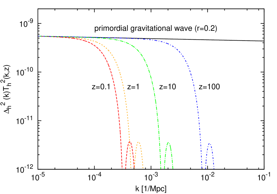
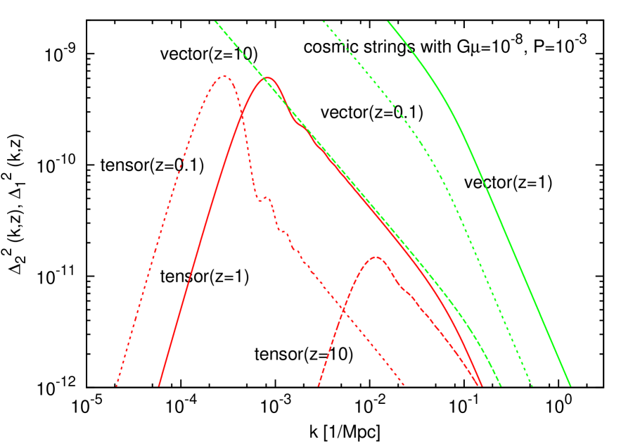
Figure 2: The dimensionless power spectrum for vector and tensor perturbations generated by primordial gravitational waves (left), a cosmic string network (right).

Based on the formulae in sec. 5.2.2 and 5.2.1, we now compute the weak lensing power spectra for the primordial gravitational waves and a cosmic string network. In Fig. 2, we first plot the dimensionless power spectra of the vector and tensor metric perturbations from the primordial gravitational waves (left) and a cosmic string network (right). Here, we specifically set the parameters to $G\mu=10^{-8}$ and $P=10^{-3}$ for the cosmic string network. Qualitatively, all the power spectra are suppressed at small scales irrespective of the type of the metric perturbations. On the other hand, large-scale behaviors are rather different, and these are sensitive to the physical properties of the seeds. For the tensor perturbations, while the scale-invariant behavior of the spectrum of primordial gravitational waves merely reflects the initial condition, a negligible contribution of the large-scale fluctuations for the cosmic string network comes from the fact that the tensor fluctuation is produced by the motion of strings, and the typical scales of their fluctuations cannot exceed the size of cosmic strings. By contrast, the vector perturbation is directly related to the velocity perturbations, whose coherent length is typically larger than the size of seeds. As a result, the spectrum of the vector perturbation for cosmic strings has a larger power, which scales as $\Delta_{1}^{2}\propto k^{-1}$ at large scales, and it dominates other perturbations.

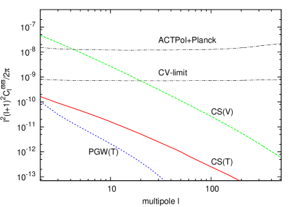
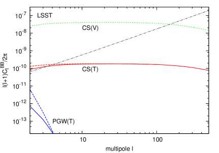
Figure 3: Left: Angular power spectra of curl-mode lensing potential from the vector and tensor perturbations, generated by the primordial gravitational waves with $r=0.2$ (PGW(T); blue dotted), and the vector (CS(V); green dashed) and the tensor (CS(T); red solid) contributions generated by the cosmic string network with $G\mu=10^{-8}$ , $P=10^{-3}$. The dot-dashed black lines represent the statistical errors coming from the reconstruction noise for the ACTPol+Planck and the CV-limit, with the maximum multipole $\ell_{\rm max}=7000$ [30] used for reconstruction analysis. Right: Angular power spectra of the B-mode cosmic shear from the primordial gravitational wave (PGW(T); blue), and the tensor (CS(T); red) and vector (CS(V); green dotted) perturbations of the cosmic string network, with (solid) and without (dashed) the metric shear/FNC term. Here, we assume the LSST survey and adopt the redshift distribution of background galaxies, (5.17). The black dot-dashed line indicates the statistical error estimated from (5.18).

The distinctive features seen in Fig. 2 basically determine the shape and amplitude of the weak lensing power spectra. Fig. 3 shows the results of the angular power spectra for curl-mode lensing potential (left) and B-mode shear (right). The model parameters of the primordial gravitational waves and cosmic string network are the same as in Fig. 2. The plotted angular power spectra are assumed to be measured from the CMB lensing experiment for the curl-mode lensing potential, and from the specific galaxy imaging survey, LSST, for the B-mode cosmic shear, respectively. That is, to compute the curl-mode power spectra, we set $\chi_{\rm S}$ to the distance to the last scattering surface, while we adopt the following redshift distribution of background galaxies for the B-mode power spectra (e.g., [64, 65]):

$$N(\chi_{\rm S})\mathrm{d}\chi_{\rm S}=N_{\mathrm{g}}\frac{3z_{\mathrm{S}}^{2}}{(0.64z_{\mathrm{m}})^{3}}\exp\biggl{[}-\left(\frac{z_{\mathrm{S}}}{0.64z_{\mathrm{m}}}\right)^{3/2}\biggr{]}\mathrm{d}z_{\mathrm{S}}\,,$$ (5.17)

with $z_{\mathrm{m}}=1.5$ and $N_{\mathrm{g}}=100\,[{\rm arcmin}^{-2}]$ .

As it is expected, the primordial gravitational waves give a negligible contribution to the lensing power spectra, and it has only a small power at lower multipoles. This is fully consistent with previous works [33, 34, 37, 38, 39]. The tensor perturbations induced by the cosmic strings are also shown to be a minor component of lensing spectrum, and it turns out that the vector perturbations from the cosmic strings can give the most dominant contribution among others. Here, for prospects of future detectability, we plot the expected statistical errors depicted as dot-dashed lines. For the curl-mode power spectrum, we consider the combination of the ground- and space-based high-resolution CMB measurements by ACTPol and Planck (ACTPol+Planck) as well as an idealistic full-sky experiment only limited by the cosmic variance (CV-limit), and calculate the statistical error arising from the lens reconstruction method (see e.g., Ref. [30]), assuming the maximum multipole $\ell_{\rm max}=7000$ used for reconstruction analysis. The statistical error for the B-mode spectrum is estimated from

$$\Delta C_{\ell}^{\mathrm{B}\mathrm{B}}=\sqrt{\frac{2}{(2\ell+1)f_{\rm sky}}}\frac{\left\langle\gamma_{\rm int}^{2}\right\rangle}{3600N_{\mathrm{g}}(180/\pi)^{2}}\,.$$ (5.18)

Assuming the LSST survey, we set the sky coverage to $f_{\rm sky}=0.5$, and adopt the empirically estimated value of the root-mean-square intrinsic ellipticity, $\left\langle\gamma_{\rm int}^{2}\right\rangle^{1/2}=0.3$ [63] . Comparison between these statistical errors and the predictions of weak lensing power spectra immediately follows that it is very difficult and challenging to detect primordial gravitational waves via the weak lensing measurement (see also Refs. [30, 34]), while a network of cosmic strings is potentially detectable through the measurement of curl-/B-mode spectrum by the vector perturbations. Although the actual impact on the detectability needs further consideration, it is found that the future weak lensing measurements have window to constrain the model parameters $G\mu$ and $P$ even tighter than the CMB observations through the Gott-Kaiser-Stebbins effect [36]. In this respect, the curl-mode and B-mode lensing spectra can be used as an important probe to find cosmic string network, and is complementary to the small-scale CMB experiment. Our full-sky formulae would be helpful for further study to explore the possibility to detect other exotic sources and to check the systematics.

6 Summary

In this paper, we present a complete set of weak lensing power spectra by scalar, vector, and tensor metric perturbations. Applying the total angular-momentum method, originally developed in the theoretical studies of CMB, we systematically derive the full-sky formulae for weak lensing observables such as the deflection angle and cosmic shear. In usual treatment of gravitational lensing, the symmetric trace-free part of the angular gradient of the deflection angle can be used as a proxy for the cosmic shear, but the relations between these variables are in general non-trivial in the presence of all types of the metric perturbations. Solving the first-order geodesic and geodesic deviation equations arising from the scalar, vector, and tensor perturbations, we have obtained the explicit gauge-invariant relation between the angular gradient of the deflection angle $\Delta_{a}$ and the cosmic shear $\gamma_{ab}$ [eq. (3.20)].

Then, based on the total angular momentum method, we presented the systematic construction of the full-sky formulae of angular power spectra for the gradient-/curl-mode lensing potential of deflection angle [eqs. (4.51)-(4.60)], and the E-/B-mode cosmic shear [eqs. (4.84)-(4.91)]. To give examples of the utility of the formulae, we have considered the weak lensing by density (scalar) perturbation, and have shown that the standard forumula for the weak lensing power spectra (i.e., gradient- and E-mode spectra) is immediately reproduced. Further, as illustrative examples for vector and tensor perturbations, we have considered the primordial gravitational waves and cosmic string network. Based on the formulae, we explicitly computed the power spectra, showing the non-vanishing signals for B-mode cosmic shear and curl-mode lensing potential. As shown in Fig. 3, the weak lensing signal by vector perturbation from cosmic strings dominates other lensing signals, and is potentially detectable from future lensing experiments for a small intercommuting probability $P\ll 1$. The framework presented here would thus be useful and helpful to explore the possibility to detect specific models for seeding non-scalar metric perturbations.

Appendix A Useful formula

In this appendix, we list some identities involving spherical Bessel function, spin-weighted spherical harmonics, intrinsic covariant derivative, and spin-operators which we have used in our calculations.

A.1 Spherical Bessel function

The spherical Bessel functions, $j_{\ell}(x)$ , are solutions to the differential equation:

$$j_{\ell}^{\prime\prime}(x)+\frac{2}{x}j_{\ell}^{\prime}(x)+\left(1-\frac{\ell(\ell+1)}{x^{2}}\right)j_{\ell}(x)=0\,.$$ (A.1)

The recursion relations of spherical Bessel functions are given by

$$\frac{j_{\ell}(x)}{x}=\frac{1}{2\ell+1}\Bigl{(}j_{\ell-1}(x)+j_{\ell+1}(x)\Bigr{)}\,,\ \ j_{\ell}^{\prime}(x)=\frac{1}{2\ell+1}\Bigl{(}\ell j_{\ell}(x)-(\ell+1)j_{\ell+1}(x)\Bigr{)}\,.$$ (A.2)

A.2 Spin-weighted spherical harmonics

To derive the spin-weighted spherical harmonics, we first introduce the spin-weighted quantities and the spin-raising/lowering operators. For a spin-$s$ function, ${}_{s}X$ , we write in terms of the spin basis and a symmetric trace-free rank-$s$ tensor, $X_{a_{1}\cdots a_{s}}$ , as

$${}_{s}X=X_{a_{1}\cdots a_{s}}e^{a_{1}}_{+}\cdots e^{a_{s}}_{+}\ \ (s\geq 0)\,,\ \ \ {}_{s}X=X_{a_{1}\cdots a_{|s|}}e^{a_{1}}_{-}\cdots e^{a_{|s|}}_{-}\ \ (s<0)\,.$$ (A.3)

Furthermore, we define a pair of operator / $\partial$ and $\bar{\ooalign{\hfil/\hfil\crcr$\partial$}}$, called spin-raising and lowering operators, respectively. These operators have the properties of increasing or decreasing the index of the spins by $1$ . For a spin-$s$ function ${}_{s}X$, these operators are defined as

$$\ooalign{\hfil/\hfil\crcr$\partial$}\left({}_{s}X\right)\equiv-\sin^{s}\theta\left(\partial_{\theta}+\frac{i}{\sin\theta}\partial_{\varphi}\right)\sin^{-s}\theta\left({}_{s}X\right)\,,$$ (A.6)

$$\bar{\ooalign{\hfil/\hfil\crcr$\partial$}}\left({}_{s}X\right)\equiv-\sin^{-s}\theta\left(\partial_{\theta}-\frac{i}{\sin\theta}\partial_{\varphi}\right)\sin^{s}\theta\left({}_{s}X\right)\,.$$ (A.9)

The spin-weighted spherical harmonics can be obtained from the spherical harmonics by applying the spin-raising and lowering operators. The spin-weighted spherical harmonics of spin weight $s=0$ are simply the standard spherical harmonics; ${}_{0}Y_{\ell}{}^{m}=Y_{\ell}{}^{m}$ . The spin-weighted spherical harmonics, ${}_{s}Y_{\ell m}$ , can be defined in terms of the spin-$0$ spherical harmonics, $Y_{\ell m}$ , as

$${}_{s}Y_{\ell}{}^{m}=\sqrt{\frac{(\ell-s)!}{(\ell+s)!}}\,\ooalign{\hfil/\hfil\crcr$\partial$}^{s}\,Y_{\ell m}\ \ (0\leq s\leq\ell)\,,$$ (A.12)

$${}_{s}Y_{\ell}{}^{m}=\sqrt{\frac{(\ell+s)!}{(\ell-s)!}}(-1)^{s}\,\bar{\ooalign{\hfil/\hfil\crcr$\partial$}}^{-s}\,Y_{\ell m}\ \ (-\ell\leq s\leq 0)\,,$$ (A.15)

and ${}_{s}Y_{\ell}{}^{m}=0$ for $\ell<|s|$ . Here we have introduced the spin-operators defined in eqs. (A.6), (A.9) . One can show that

$$\ooalign{\hfil/\hfil\crcr$\partial$}\,{}_{s}Y_{\ell}{}^{m}=\sqrt{(\ell-s)(\ell+s+1)}\,{}_{s+1}Y_{\ell}{}^{m}\,,\ \ \bar{\ooalign{\hfil/\hfil\crcr$\partial$}}\,{}_{s}Y_{\ell}{}^{m}=-\sqrt{(\ell+s)(\ell-s+1)}\,{}_{s-1}Y_{\ell}{}^{m}\,.$$ (A.20)

Since the spin-$0$ , $\pm 1$ , $\pm 2$ harmonics are useful in this paper, we give their explicit form in Tables 2 and 3 . The spin-weighted spherical harmonics satisfy the conjugate relation $({}_{s}Y_{\ell}{}^{m})^{*}=(-1)^{m+s}{}_{-s}Y_{\ell}{}^{-m}$ , the parity relation ${}_{s}Y_{\ell}{}^{m}(\pi-\theta,\phi-\pi)=(-1)^{\ell}{}_{-s}Y_{\ell}{}^{m}(\theta,\phi)$ , the orthonormal relationship

$$\int\mathrm{d}\Omega\,\bigl{(}{}_{s}Y_{\ell^{\prime}}{}^{m^{\prime}}\bigr{)}^{*}{}_{s}Y_{\ell}{}^{m}=\delta_{\ell\ell^{\prime}}\delta_{mm^{\prime}}\,,$$ (A.21)

the completeness relation

$$\sum_{\ell=1}^{\infty}\sum_{m=-\ell}^{\ell}\,\bigl{(}{}_{s}Y_{\ell}{}^{m}(\theta^{\prime},\phi^{\prime})\bigr{)}^{*}\,{}_{s}Y_{\ell}{}^{m}(\theta,\phi)=\delta_{\mathrm{D}}(\cos\theta-\cos\theta^{\prime})\delta_{\mathrm{D}}(\phi-\phi^{\prime})\,,$$ (A.22)

the addition relation

$$\sum_{m}\bigl{(}{}_{s_{1}}Y_{\ell}{}^{m}(\theta^{\prime},\phi^{\prime})\bigr{)}^{*}\,{}_{s_{2}}Y_{\ell}{}^{m}(\theta,\phi)=\sqrt{\frac{2\ell+1}{4\pi}}{}_{s_{2}}Y_{\ell}{}^{-s_{1}}(\beta,\alpha)e^{-is_{2}\gamma}\,,$$ (A.23)

where $(\alpha,\beta,\gamma)$ relates the rotation from $(\theta^{\prime},\phi^{\prime})$ through the origin to $(\theta,\phi)$ , the Clebsch-Gordan relation

$${}_{s_{1}}Y_{\ell_{1}}{}^{m_{1}}\,{}_{s_{2}}Y_{\ell_{2}}{}^{m_{2}}= \frac{\sqrt{(2\ell_{1}+1)(2\ell_{2}+1)}}{4\pi}\sum_{\ell,m,s}\langle\ell_{1},\ell_{2};m_{1},m_{2}|\ell_{1},\ell_{2};\ell,m\rangle$$

$$\quad\quad\quad\times\langle\ell_{1},\ell_{2};-s_{1},-s_{2}|\ell_{1},\ell_{2};\ell,-s\rangle\sqrt{\frac{4\pi}{2\ell+1}}{}_{s}Y_{\ell}{}^{m}\,,$$ (A.24)

where $\langle\ell_{1},\ell_{2};m_{1},m_{2}|\ell,m\rangle$ denotes the Clebsch-Gordan coefficient.

Table 2: Spin-$0$, $1$, $2$ spherical harmonics for $\ell=1$ .

$m$	${}_{0}Y_{1}{}^{m}$	${}_{+1}Y_{1}{}^{m}$	${}_{+2}Y_{1}{}^{m}$
$0$	$\sqrt{\frac{3}{4\pi}}\mu$	$\sqrt{\frac{3}{8\pi}}\sqrt{1-\mu^{2}}$	$0$
$\pm 1$	$\mp\sqrt{\frac{3}{8\pi}}\sqrt{1-\mu^{2}}e^{\pm i\varphi}$	$-\sqrt{\frac{3}{16\pi}}(1\mp\mu)e^{\pm i\varphi}$	$0$
$\pm 2$	$0$	$0$	$0$

Table 3: Spin-$0$, $1$, $2$ spherical harmonics for $\ell=2$ .

$m$	${}_{0}Y_{2}{}^{m}$	${}_{+1}Y_{2}{}^{m}$	${}_{+2}Y_{2}{}^{m}$
$0$	$\sqrt{\frac{5}{16\pi}}(3\mu^{2}-1)$	$\sqrt{\frac{15}{8\pi}}\mu\sqrt{1-\mu^{2}}$	$\sqrt{\frac{15}{32\pi}}(1-\mu^{2})$
$\pm 1$	$\mp\sqrt{\frac{15}{8\pi}}\mu\sqrt{1-\mu^{2}}e^{\pm i\varphi}$	$-\sqrt{\frac{5}{16\pi}}(1\mp\mu)(2\mu\pm 1)e^{\pm i\varphi}$	$\sqrt{\frac{5}{16\pi}}\sqrt{1-\mu^{2}}(1\mp\mu)e^{\pm i\varphi}$
$\pm 2$	$\sqrt{\frac{15}{32\pi}}(1-\mu^{2})e^{\pm 2i\varphi}$	$-\sqrt{\frac{5}{16\pi}}\sqrt{1-\mu^{2}}\left(\mu\mp 1\right)e^{\pm 2i\varphi}$	$\sqrt{\frac{5}{64\pi}}\left(1\mp\mu\right)^{2}e^{\pm 2i\varphi}$

A.3 Intrinsic covariant derivative and spin operators

In this subsection, we describe the basis vectors in the explicit Cartesian coordinate and define the spin-raising/lowering operators, and present the relation between the intrinsic covariant derivative on the unit sphere and the spin operators. When we consider a static observer, $u^{\mu}=(1,{\bm{0}})$ , the three-dimensional spatial basis vectors , $\hat{\bm{n}}$ and ${\bm{e}}_{a}$ , can be described explicitly in terms of the Cartesian coordinate as

$$\hat{\bm{n}}=\left(\sin\theta\cos\varphi,\sin\theta\sin\varphi,\cos\theta\right)\,,$$ (A.25)

$${\bm{e}}_{\theta}(\hat{\bm{n}})=\left(\cos\theta\cos\varphi,\cos\theta\sin\varphi,-\sin\theta\right)\,,$$ (A.26)

$${\bm{e}}_{\varphi}(\hat{\bm{n}})=\left(-\sin\theta\sin\varphi,\sin\theta\cos\varphi,0\right)\,.$$ (A.27)

With these notations, we have

$$\hat{n}^{i}\partial_{i}=\partial_{\chi}\,,\ \ e^{i}_{\theta}\partial_{i}=\chi^{-1}\partial_{\theta}\,,\ \ e^{i}_{\varphi}=\chi^{-1}\partial_{\varphi}\,,$$ (A.28)

and we can evaluate

$$\chi\,\hat{\bm{n}}_{|j}e^{j}_{a}={\bm{e}}_{a}\,,\ \ \chi^{2}\,\hat{\bm{n}}_{|jk}e^{j}_{(a}e^{k}_{b)}=-\omega_{ab}\,\hat{\bm{n}}\,,\ \ {\bm{e}}_{a|j}\hat{n}^{j}=0\,,$$ (A.29)

$$\chi\,{\bm{e}}_{\theta|j}e^{j}_{\varphi}=\chi{\bm{e}}_{\varphi|j}e^{j}_{\theta}=\cot\theta\,{\bm{e}}_{\varphi}\,,\ \ \chi\,{\bm{e}}_{\theta|j}e^{j}_{\theta}=-\hat{\bm{n}}\,,$$ (A.30)

$$\chi\,{\bm{e}}_{\varphi|j}e^{j}_{\varphi}=-\sin\theta\left(\sin\theta\,\hat{\bm{n}}+\cos\theta\,{\bm{e}}_{\theta}\right)\,.$$ (A.31)

We then derive the explicit relation between the covariant derivative of a two-vector on the unit sphere and the three-dimensional covariant derivative:

$$X_{a:b}=\chi(X_{i}e^{i}_{a})_{|j}e^{j}_{b}-{}^{(2)}\Gamma^{c}_{ab}X_{i}e^{i}_{c}\,,\ \ \ {}^{(2)}\Gamma^{c}_{ab}=\chi e^{i}_{a|j}e^{j}_{b}e^{c}_{i}\,,$$ (A.32)

where ${}^{(2)}\Gamma^{c}_{ab}$ denotes the Christoffel symbol defined on the unit sphere. Here the polarization indices are raised or lowered with respect to $\omega_{ab}$ . With a help of eqs. (A.30) and (A.31) , one can easily verify the following relations:

$$e_{\pm}^{a}{}_{:b}\,e_{\pm}^{b}=\cot\theta\,e_{\pm}^{a}\,,\ \ \ e_{\pm}^{a}{}_{:b}\,e_{\mp}^{b}=-\cot\theta\,e_{\pm}^{a}\,.$$ (A.33)

These equations can be used to construct the explicit relations between the intrinsic covariant derivative and spin-raising/lowering operators. Using eqs. (A.33), one can verify the explicit relations such as ${}_{0}X_{:ab}e^{a}_{+}e^{b}_{-}=\ooalign{\hfil/\hfil\crcr$\partial$}\bar{\ooalign{\hfil/\hfil\crcr$\partial$}}\left({}_{0}X\right)$ , $X_{a:b}e^{a}_{+}e^{b}_{+}=-\ooalign{\hfil/\hfil\crcr$\partial$}\left({}_{+1}X\right)$ and so on, which we have used in our calculations.

Appendix B Christoffel symbols and Riemann tensors

Christoffel symbols and Riemann tensor on the unperturbed spacetime in the Cartesian coordinate system are trivially $\Gamma^{\rho}_{\mu\nu}=0$ , and $R_{\mu\rho\nu\sigma}=0$ . Since the Christoffel symbols are not covariant quantities, the unperturbed Christoffel symbols in the spherical coordinate system can have the non-vanishing components:

$$\Gamma^{\chi}_{ab}=-\chi\omega_{ab}\,,\ \Gamma^{a}_{\chi b}=\frac{1}{\chi}\delta^{a}{}_{b}\,,\ \Gamma^{a}_{bc}=^{(2)}\Gamma^{a}_{bc}\,,\ \text{otherwise}=0\,,$$ (B.1)

where $a,b,c=\theta,\varphi$ and the two-dimensional Christoffel symbols are given by

$${}^{(2)}\Gamma^{\theta}_{\varphi\varphi}=-\sin\theta\cos\theta\,,\ \ \ ^{(2)}\Gamma^{\varphi}_{\theta\varphi}=\cot\theta\,,\ \ \ \text{otherwise}=0\,.$$ (B.2)

Using the explicit expression for the linearized Christoffel symbols, $\delta\Gamma^{\rho}_{\mu\nu}=\frac{1}{2}g^{\rho\sigma}(\delta g_{\sigma\mu;\nu}+\delta g_{\sigma\nu;\mu}-\delta g_{\mu\nu;\sigma})$ , we can calculate the components of the linearized Christoffel symbols as

$$\delta\Gamma^{0}_{00}=\dot{A}\,,\ \ \delta\Gamma^{0}_{0i}=A_{|i}\,,\ \ \delta\Gamma^{i}_{00}=A^{|i}+\dot{\tilde{B}}^{i}\,,\ \ \delta\Gamma^{0}_{ij}=-\tilde{B}_{(i|j)}+\frac{1}{2}\dot{\tilde{H}}_{ij}\,,$$ (B.3)

$$\delta\Gamma^{i}_{0j}=\frac{1}{2}\left(\tilde{B}^{i}{}_{|j}-\tilde{B}_{j}{}^{|i}\right)+\frac{1}{2}\dot{\tilde{H}}^{i}{}_{j}\,,\ \ \delta\Gamma^{i}_{jk}=\frac{1}{2}\bar{\gamma}^{il}\left(\tilde{H}_{jl|k}+\tilde{H}_{kl|j}-\tilde{H}_{jk|l}\right)\,,$$ (B.4)

where we have introduced $\tilde{B}_{i}\equiv\delta g_{0i}$ and $\tilde{H}_{ij}\equiv\delta g_{ij}$ for simplicity. With a help of the geodesic in the unperturbed spacetime, $x^{\mu}=(\eta_{0}-\chi,\chi\hat{\bm{n}})$ , and using the formulas (A.28)-(A.31) , we obtain the angular component of the linearized Christoffel symbols in terms of the gauge-invariant variables defined in eqs. (2.5)-(2.7) as

$$e_{i}^{a}\delta\Gamma^{i}_{\mu\nu}\frac{\mathrm{d}x^{\mu}}{\mathrm{d}\chi}\frac{\mathrm{d}x^{\nu}}{\mathrm{d}\chi}= \frac{1}{\chi}\omega^{ab}\biggl{\{}\Upsilon_{:b}+\frac{\mathrm{d}}{\mathrm{d}\chi}\bigl{(}\chi\Omega_{b}\bigr{)}\biggr{\}}\,,$$ (B.5)

where we have introduced the spin-$0$ and $1$ combinations of the gauge-invariants:

$$\Upsilon\equiv\Psi-\Phi+\sigma_{\mathrm{g},i}\hat{n}^{i}+\frac{1}{2}h_{ij}\hat{n}^{i}\hat{n}^{j}\,,\ \ \Omega_{i}\equiv\sigma_{\mathrm{g},i}+h_{ij}\hat{n}^{j}\,.$$ (B.6)

We can calculate the linearized Riemann tensor as $\delta R_{\mu\rho\nu\sigma}=\frac{1}{2}(-\delta g_{\mu\nu;\rho\sigma}-\delta g_{\rho\sigma;\mu\nu}+\delta g_{\mu\sigma;\rho\nu}+\delta g_{\nu\rho;\mu\sigma})$ . We have the non-vanishing components of the linearized Riemann tensor as

$$\delta R_{0i0j}=-A_{|ij}+\tilde{B}_{(i|j)}-\frac{1}{2}\ddot{\tilde{H}}_{ij}\,,\ \ \delta R_{ij0k}=-\tilde{B}_{[i|j]k}-\dot{\tilde{H}}_{k[i|j]}\,,$$ (B.7)

$$\delta R_{ikj\ell}=\frac{1}{2}\left(-\tilde{H}_{ij|k\ell}-\tilde{H}_{k\ell|ij}+\tilde{H}_{i\ell|kj}+\tilde{H}_{jk|i\ell}\right)\,.$$ (B.8)

Substituting these non-vanishing Riemann tensor into eq. (3.14) , and using the relations between the basis vectors (A.28)-(A.31) , we have the explicit expression for the perturbed symmetric optical tidal matrix, $\delta\mathcal{T}_{ab}$ , induced by the scalar, vector, and tensor perturbations:

$$\chi^{2}\delta\mathcal{T}_{ab}= \Upsilon_{:ab}-\frac{\mathrm{d}}{\mathrm{d}\chi}\bigl{(}\chi\Omega_{(a:b)}\bigr{)}+\frac{1}{2}\chi\frac{\mathrm{d}^{2}}{\mathrm{d}\chi^{2}}\bigl{(}\chi h_{ab}\bigr{)}+\chi\omega_{ab}\biggl{\{}\partial_{\chi}\Upsilon-\frac{\mathrm{d}}{\mathrm{d}\chi}\left(\Omega_{i}\hat{n}^{i}\right)+\chi\frac{\mathrm{d}^{2}}{\mathrm{d}\chi^{2}}\mathcal{R}\biggr{\}}\,,$$ (B.9)

where $h_{ab}\equiv h_{ij}e^{i}_{a}e^{j}_{b}$ , $\Omega_{a}\equiv\Omega_{i}e^{i}_{a}$ , and we have defined $\Upsilon$ , $\Omega_{i}$ in eq. (B.6) . We should note that the gauge degree of freedom is not completely removed in the symmetric optical tidal matrix (B.9) . At first-order, however, the contributions from the residual gauge freedom affects only the trace part of the symmetric optical tidal matrix. Hence, it is necessary to consider the other contributions when we take the trace part of the Jacobi map into account.

Appendix C ${}_{s}\epsilon_{L}^{(\ell,m)}$ and ${}_{s}\beta_{L}^{(\ell,m)}$

In this section we will present the explicit expression for ${}_{s}\epsilon_{L}^{(\ell,m)}$ and ${}_{s}\beta_{L}^{(\ell,m)}$ . We are only interested in the cases of $s=0$ , $\pm 1$ , $\pm 2$ . Using the Clebsch-Gordan coefficients and the recurrent relations of spherical Bessel functions presented in Appendix A.1 , we obtain

$${}_{0}\epsilon_{L}^{(0,0)}(x)=j_{L}(x)\,,\ \ \ {}_{0}\epsilon_{L}^{(1,0)}(x)=j_{L}^{\prime}(x)\,,\ \ \ {}_{0}\epsilon_{L}^{(1,\pm 1)}(x)=\sqrt{\frac{L(L+1)}{2}}\frac{j_{L}(x)}{x}\,,$$ (C.1)

$${}_{0}\epsilon_{L}^{(2,0)}(x)=\frac{1}{2}\left(3j_{L}^{\prime\prime}(x)+j_{L}(x)\right)\,,\ \ \ {}_{0}\epsilon_{L}^{(2,\pm 1)}(x)=\sqrt{\frac{3L(L+1)}{2}}\left(\frac{j_{L}(x)}{x}\right)^{\prime}\,,$$ (C.2)

$${}_{0}\epsilon_{L}^{(2,\pm 2)}(x)=\sqrt{\frac{3(L+2)!}{8(L-2)!}}\frac{j_{L}(x)}{x^{2}}\,,\ \ \ {}_{0}\beta_{L}^{(\ell,m)}(x)=0\ \ (\ell=0\,,1\,,2)\,,$$ (C.3)

for $s=0$ ,

$${}_{1}\epsilon_{L}^{(1,0)}(x)=\sqrt{\frac{L(L+1)}{2}}\frac{j_{L}(x)}{x}\,,\ \ \ {}_{1}\epsilon_{L}^{(1,\pm 1)}(x)=\frac{1}{2}\left(\frac{j_{L}(x)}{x}+j_{L}^{\prime}(x)\right)\,,$$ (C.4)

$${}_{1}\epsilon_{L}^{(2,0)}(x)=\sqrt{\frac{3L(L+1)}{2}}\left(\frac{j_{L}(x)}{x}\right)^{\prime}\,,$$ (C.5)

$${}_{1}\epsilon_{L}^{(2,\pm 1)}(x)=\frac{1}{2}\left(j_{L}(x)+2j_{L}^{\prime\prime}(x)-2\frac{j_{L}(x)}{x^{2}}+\frac{2}{x}j_{L}^{\prime}(x)\right)\,,$$ (C.6)

$${}_{1}\epsilon_{L}^{(2,\pm 2)}(x)=\frac{1}{2}\sqrt{(L-1)(L+2)}\left(\frac{j_{L}(x)}{x^{2}}+\frac{j_{L}^{\prime}(x)}{x}\right)\,,$$ (C.7)

$${}_{1}\beta_{L}^{(1,0)}(x)=0\,,\ \ \ {}_{1}\beta_{L}^{(1,\pm 1)}(x)=\pm\frac{1}{2}j_{L}(x)\,,$$ (C.8)

$${}_{1}\beta_{L}^{(2,0)}(x)=0\,,\ \ \ {}_{1}\beta_{L}^{(2,\pm 1)}(x)=\pm\frac{1}{2}\left(j_{L}^{\prime}(x)-\frac{j_{L}(x)}{x}\right)\,,$$ (C.9)

$${}_{1}\beta_{L}^{(2,\pm 2)}(x)=\pm\frac{1}{2}\sqrt{(L-1)(L+2)}\frac{j_{L}(x)}{x}\,,$$ (C.10)

for $s=\pm 1$ , and

$${}_{2}\epsilon_{L}^{(2,0)}(x)=\sqrt{\frac{3(L+2)!}{8(L-2)!}}\frac{j_{L}(x)}{x^{2}}\,,$$ (C.11)

$${}_{2}\epsilon_{L}^{(2,\pm 1)}(x)=\frac{1}{2}\sqrt{(L-1)(L+2)}\left(\frac{j_{L}(x)}{x^{2}}+\frac{j_{L}^{\prime}(x)}{x}\right)\,,$$ (C.12)

$${}_{2}\epsilon_{L}^{(2,\pm 2)}(x)=\frac{1}{4}\left(-j_{L}(x)+j_{L}^{\prime\prime}(x)+2\frac{j_{L}(x)}{x^{2}}+4\frac{j_{L}^{\prime}(x)}{x}\right)\,,$$ (C.13)

$${}_{2}\beta_{L}^{(2,0)}(x)=0\,,\ \ \ {}_{2}\beta_{L}^{(2,\pm 1)}(x)=\pm\frac{1}{2}\sqrt{(L-1)(L+2)}\frac{j_{L}(x)}{x}\,,$$ (C.14)

$${}_{2}\beta_{L}^{(2,\pm 2)}(x)=\pm\frac{1}{2}\left(j_{L}^{\prime}(x)+2\frac{j_{L}(x)}{x}\right)\,,$$ (C.15)

for $s=\pm 2$ .

Appendix D Derivation of correlations of a cosmic string network

In this section, we derive the auto-power spectrum for the non-vanishing vector and tensor modes of the string stress-energy tensor. We first briefly review an analytic model for the correlation between string segments in section D.1 . In section D.2 and D.3, we derive the analytic expression for the auto-power spectrum for the vector and tensor perturbations induced by the cosmic string network.

D.1 String correlators

To evaluate the auto-power spectrum for the non-vanishing stress-energy tensor, we write down the string stress-energy tensor. The stress-energy tensor for a string segment in the transverse gauge is described as

$$\delta T^{\mu\nu}({\bm{r}},\eta)=\mu\int\mathrm{d}\sigma\left(\begin{array}[]{cc}1&-\dot{r}^{i}\\ -\dot{r}^{j}&\dot{r}^{i}\dot{r}^{j}-{r^{i}}^{\prime}{r^{j}}^{\prime}\\ \end{array}\right)\delta_{\mathrm{D}}^{3}({\bm{r}}-{\bm{r}}(\sigma,\eta))\,,$$ (D.1)

where the dot ( $\dot{}$ ) and the prime ( ^′ ) denote the derivative with respect to $\eta$ and $\sigma$ , respectively. Hereafter, we use a simple model to compute the string correlations developed in Refs. [61, 62, 60]. We assume that all correlations can be expressed in terms of the two point functions: $\langle\dot{r}^{i}(\sigma_{1},\eta)\dot{r}^{j}(\sigma_{2},\eta)\rangle\,,\ \langle{r^{i}}^{\prime}(\sigma_{1},\eta){r^{j}}^{\prime}(\sigma_{2},\eta)\rangle\,,\ \langle{r^{i}}^{\prime}(\sigma_{1},\eta)\dot{r}^{j}(\sigma_{2},\eta)\rangle$ . Furthermore,these two point functions are assumed to be exactly Gaussian and isotropic is assumed to be distributed with mean zero and following variances:

$$\big{\langle}\dot{r}^{i}(\sigma_{1},\eta)\dot{r}^{j}(\sigma_{2},\eta)\big{\rangle}=\frac{1}{3}\delta^{ij}\,V_{\rm s}(\sigma_{1}-\sigma_{2},\eta)\,,$$ (D.2)

$$\big{\langle}{r^{i}}^{\prime}(\sigma_{1},\eta){r^{j}}^{\prime}(\sigma_{2},\eta)\big{\rangle}=\frac{1}{3}\delta^{ij}\,T_{\rm s}(\sigma_{1}-\sigma_{2},\eta)\,,$$ (D.3)

$$\big{\langle}{r^{i}}^{\prime}(\sigma_{1},\eta)\dot{r}^{j}(\sigma_{2},\eta)\big{\rangle}=\frac{1}{3}\delta^{ij}\,M_{\rm s}(\sigma_{1}-\sigma_{2},\eta)\,.$$ (D.4)

Since in our calculation we consider only a segment of a long string with length $\xi$ , the correlators are expected to be damped on scale larger than the correlation length, namely $\sigma\gg\xi/a$ , and have the non-vanishing expectation value on $\sigma\ll\xi/a$. Hence the asymptotic forms are [60]

$$T_{\rm s}(\sigma,\eta)=\Biggl{\{}\begin{array}[]{ll}\bar{t}^{2}&:\ \sigma\ll\xi/a\\ 0&:\ \sigma\gg\xi/a\\ \end{array}\,,$$ (D.7)

$$V_{\rm s}(\sigma,\eta)=\Biggl{\{}\begin{array}[]{ll}\bar{v}^{2}&:\ \sigma\ll\xi/a\\ 0&:\ \sigma\gg\xi/a\\ \end{array}\,,$$ (D.10)

$$M_{\rm s}(\sigma,\eta)=\Biggl{\{}\begin{array}[]{ll}ac_{0}\sigma/\xi&:\ \sigma\ll\xi/a\\ 0&:\ \sigma\gg\xi/a\\ \end{array}\,,$$ (D.13)

where we have introduced the three parameters: $\bar{t}^{2}\equiv\big{\langle}{{\bm{r}}^{\prime}}^{2}\big{\rangle}\,,\ \bar{v}^{2}\equiv\left\langle\dot{\bm{r}}^{2}\right\rangle\,,\ c_{0}\equiv\frac{\xi}{a}\left\langle\dot{\bm{r}}\cdot{\bm{r}}^{\prime\prime}\right\rangle$ . We can evaluate the parameters as

$$\bar{t}\approx\sqrt{1-v_{\rm rms}^{2}}\,,\ \ \bar{v}\approx v_{\rm rms}\,,\ \ c_{0}\approx\frac{2\sqrt{2}}{\pi}v_{\rm rms}\left(1-v_{\rm rms}^{2}\right)\frac{1-8v_{\rm rms}^{6}}{1+8v_{\rm rms}^{6}}\,.$$ (D.14)

Once $\xi$ and $v_{\rm rms}$ are properly evaluated through the string network model, they fix the parameters used to calculate the correlators.

D.2 Vector mode

We provide brief summary of the method to calculate the auto-power spectrum for the vector perturbations in the conformal Newton gauge, following [36]. The vector-type fluctuation for the stress-energy tensor can be decomposed into the vector mode functions defined in section 4.2 as

$$\delta T^{0}{}_{i}({\bm{x}},\eta)=\int\frac{\mathrm{d}^{3}{\bm{k}}}{(2\pi)^{3}}\sum_{m=\pm 1}v_{\bm{k}}^{(m)}(\eta)\,Q^{(m)}_{i}({\bm{x}},{\bm{k}})\,.$$ (D.15)

Comparing to eqs. (D.15) and (D.1) , we obtain the vector-type perturbations , $v_{\bm{k}}^{(\pm 1)}(\eta)$ , due to a string segment:

$$v_{\bm{k}}^{(\pm 1)}(\eta)=\frac{\mu}{\sqrt{2}i}\int\mathrm{d}\sigma\,{\bm{e}}_{\pm}^{*}(\hat{\bm{k}})\cdot\dot{\bm{r}}(\sigma,\eta)e^{-i{\bm{k}}\cdot{\bm{r}}(\sigma,\eta)}\,.$$ (D.16)

We assume that the total correlations can be described by a summation of the contribution of each segment and the correlations between the different segments are negligibly small. The linearized Einstein equation implies that the auto-power spectrum for vector metric perturbations induced by the string network can be approximated as

$$\Delta_{1}^{2}(k,\eta) =\frac{k^{3}}{2\pi^{2}}\frac{(16\pi G)^{2}a^{4}}{k^{4}}n_{\rm s}\delta V\frac{1}{\mathcal{V}}\left\langle\left(v_{\bm{k}}^{(\pm 1)}(\eta)\right)^{*}v_{\bm{k}}^{(\pm 1)}(\eta)\right\rangle$$

$$=\frac{(16G)^{2}a^{4}}{4k}n_{\rm s}\delta V\frac{1}{\mathcal{V}}\int\mathrm{d}\sigma_{1}\mathrm{d}\sigma_{2}\left(e^{(\pm 1)}_{i}(\hat{\bm{k}})\right)^{*}e^{(\pm 1)}_{j}(\hat{\bm{k}})$$

$$\quad\quad\quad\quad\times\left\langle\dot{r}^{i}(\sigma_{1},\eta)\dot{r}^{j}(\sigma_{2},\eta)\exp\biggl{[}i{\bm{k}}\cdot\left({\bm{r}}(\sigma_{1},\eta)-{\bm{r}}(\sigma_{2},\eta)\right)\biggr{]}\right\rangle\,,$$ (D.17)

where $\delta V=4\pi\chi^{2}/H$ is the comoving differential volume element, $n_{\rm s}=a^{3}\xi^{-3}$ is the comoving number density of the string segments, and $\mathcal{V}\equiv(2\pi)^{3}\delta_{\mathrm{D}}^{3}({\bm{0}})$ is the comoving box size . Using the correlators (D.2)-(D.4) , we can compute the equal-time auto-power spectrum for the tensor perturbations as

$$\Delta_{1}^{2}(k,\eta)=\frac{(16G\mu)^{2}a^{4}}{24k}n_{\rm s}\delta V\frac{1}{\mathcal{V}}\int\mathrm{d}\sigma_{+}\mathrm{d}\sigma_{-}V_{\rm s}(\sigma_{-},\eta)\exp\biggl{[}-\frac{1}{6}k^{2}\Gamma_{\rm s}(\sigma_{-},\eta)\biggr{]}\,,$$ (D.18)

where $\sigma_{\pm}=\sigma_{1}\pm\sigma_{2}$ and we have introduced $\Gamma_{\rm s}$ defined as

$$\Gamma_{\rm s}(\sigma_{1}-\sigma_{2},\eta)\equiv\left\langle\Bigl{\{}{\bm{r}}(\sigma_{1},\eta)-{\bm{r}}(\sigma_{2},\eta)\Bigr{\}}^{2}\right\rangle=\int^{\sigma_{1}}_{\sigma_{2}}\mathrm{d}\sigma_{3}\mathrm{d}\sigma_{4}\,T_{\rm s}(\sigma_{3}-\sigma_{4},\eta)\,.$$ (D.19)

The asymptotic behavior of $T_{\rm s}$, eq. (D.7) , leads to $\Gamma_{\rm s}\approx\bar{t}^{2}\sigma^{2}$ on scalar smaller than the correlation length. Since the term $\int\mathrm{d}\sigma_{+}/\mathcal{V}$ corresponds to the length of the string segment within the unit volume and the correlators are damped at $\sigma\gg\xi/a$ , we can take the region of the integration as $\int\mathrm{d}\sigma_{+}/\mathcal{V}=a^{2}/\xi^{2}\sqrt{1-v_{\rm rms}^{2}}$ and $|\sigma_{-}|<\xi/2a\sqrt{1-v_{\rm rms}^{2}}$. We then have

$$\Delta_{1}^{2}(k,\eta)=\left(16G\mu\right)^{2}\frac{\sqrt{6\pi}\,v_{\rm rms}^{2}}{12(1-v_{\rm rms}^{2})}\frac{4\pi k^{3}\chi^{2}a^{4}}{H}\left(\frac{a}{k\xi}\right)^{5}{\rm erf}\left(\frac{k\xi/a}{2\sqrt{6}}\right)\,.$$ (D.20)

D.3 Tensor mode

For tensor-components, the fluctuation can be decomposed into the tensor mode functions defined in section 4.2 as

$$\delta T^{i}{}_{j}({\bm{x}},\eta)=\int\frac{\mathrm{d}^{3}{\bm{k}}}{(2\pi)^{3}}\sum_{m=\pm 2}\Pi_{\bm{k}}^{(m)}(\eta)\,Q^{(m)}{}^{i}{}_{j}({\bm{x}},{\bm{k}})\,.$$ (D.21)

Comparing to eqs. (D.1) and (D.21) , the tensor-type perturbations due to a string segment, $\Pi_{\bm{k}}^{(\pm 2)}(\eta)$ , are given by

$$\Pi_{\bm{k}}^{(\pm 2)}(\eta)= -\frac{1}{2\sqrt{2}}\,\mu\int\mathrm{d}\sigma\left\{\dot{r}^{i}(\sigma,\eta)\dot{r}^{j}(\sigma,\eta)-{r^{i}}^{\prime}(\sigma,\eta){r^{j}}^{\prime}(\sigma,\eta)\right\}e_{\pm,i}^{*}(\hat{\bm{k}})e_{\pm,j}^{*}(\hat{\bm{k}})\,e^{i{\bm{k}}\cdot{\bm{r}}(\sigma,\eta)}\,.$$ (D.22)

Assuming that the auto-power spectra for the fluctuation of the stress-energy tensor have the form:

$$\left\langle\bigl{(}\Pi_{\bm{k}}^{(m)}(\eta)\bigr{)}^{*}\Pi_{{\bm{k}}^{\prime}}^{(m^{\prime})}(\eta^{\prime})\right\rangle=(2\pi)^{3}\delta_{\mathrm{D}}^{3}({\bm{k}}-{\bm{k}}^{\prime})\delta_{mm^{\prime}}\frac{2\pi^{2}}{k^{3}}\Delta_{\Pi}(k,\eta)\Delta_{\Pi}(k,\eta^{\prime})\,,$$ (D.23)

we can describe the auto-power spectrum for the tensor perturbations in terms of the auto-power spectrum for the tensor component of the stress-energy as

$$\Delta_{2}(k,\eta)=\int^{\eta}k\,\mathrm{d}\eta^{\prime}\,\mathcal{G}(k\eta,k\eta^{\prime})\,\mathcal{K}(k,\eta^{\prime})\,.$$ (D.24)

where $\mathcal{G}$ is the Green function for the equation (5.8) and $\mathcal{K}$ is the kernel defined by

$$\mathcal{K}(k,\eta)\equiv\frac{8\pi Ga^{2}(\eta)}{k^{2}}\Delta_{\Pi}(k,\eta)\,.$$ (D.25)

With a help of the correlators eqs.  (D.2)-(D.4) and (D.19) , we can evaluate the auto-power spectrum for $\Pi$ as

$$\Delta_{\Pi}^{2}(k,\eta)=\frac{k^{3}}{2\pi^{2}}n_{\rm s}\delta V\frac{1}{\mathcal{V}}\left\langle{\Pi_{\bm{k}}^{(\pm 2)}}^{*}(\eta)\Pi_{\bm{k}}^{(\pm 2)}(\eta)\right\rangle$$

$$\quad=\frac{k^{3}\mu^{2}}{16\pi^{2}}n_{\rm s}\delta V\frac{1}{\mathcal{V}}\int\mathrm{d}\sigma_{1}\mathrm{d}\sigma_{2}\,e_{\pm,i}^{*}(\hat{\bm{k}})e_{\pm,j}^{*}(\hat{\bm{k}})e_{\pm,k}(\hat{\bm{k}})e_{\pm,\ell}(\hat{\bm{k}})\,$$

$$\quad\quad\times\Big{\langle}\left\{\dot{r}^{i}(\sigma_{1},\eta)\dot{r}^{j}(\sigma_{1},\eta)-{r^{i}}^{\prime}(\sigma_{1},\eta){r^{j}}^{\prime}(\sigma_{1},\eta)\right\}\left\{\dot{r}^{k}(\sigma_{2},\eta)\dot{r}^{\ell}(\sigma_{2},\eta)-{r^{k}}^{\prime}(\sigma_{2},\eta){r^{\ell}}^{\prime}(\sigma_{2},\eta)\right\}$$

$$\quad\quad\quad\quad\times\exp\Bigl{[}-i{\bm{k}}\cdot\Bigl{(}{\bm{r}}(\sigma_{1},\eta)-{\bm{r}}(\sigma_{2},\eta)\Bigr{)}\Bigr{]}\Bigr{\rangle}\,.$$ (D.26)

With a help of the correlators defined in eqs. (D.2)-(D.4) , we can compute the equal-time auto-power spectrum for the tensor-type perturbations as

$$\Delta_{\Pi}^{2}(k,\eta)= \frac{k^{3}\mu^{2}}{36\pi^{2}}n_{\rm s}\delta V\frac{1}{\mathcal{V}}\int\mathrm{d}\sigma_{+}\mathrm{d}\sigma_{-}$$

$$\quad\times\biggl{(}T_{\rm s}^{2}(\sigma_{-},\eta)+V_{\rm s}^{2}(\sigma_{-},\eta)-2M_{\rm s}^{2}(\sigma_{-},\eta)\biggr{)}\exp\left(-\frac{1}{6}k^{2}\Gamma(\sigma_{-},\eta)\right)\,,$$ (D.27)

where $\sigma_{\pm}\equiv\sigma_{1}\pm\sigma_{2}$ and we have defined $\Gamma_{\rm s}$ in eq. (D.19) . As discussed in previous subsection D.2, taking the region of the integration as $\int\mathrm{d}\sigma_{+}/\mathcal{V}=a^{2}/\xi^{2}\sqrt{1-v_{\rm rms}^{2}}$ and $|\sigma_{-}|<\xi/2a\sqrt{1-v_{\rm rms}^{2}}$ , we have the kernel $\mathcal{K}$ induced by the string network:

$$\mathcal{K}^{2}(k,\eta)\approx \frac{\sqrt{6\pi}(8G\mu)^{2}}{36\sqrt{1-v_{\rm rms}^{2}}}\frac{4\pi k^{3}\chi^{2}a^{4}}{H}\left(\frac{a}{k\xi}\right)^{5}\Biggl{[}\Big{\{}(1-v_{\rm rms}^{2})^{2}+v^{4}_{\rm rms}\Bigr{\}}{\rm erf}\left(\frac{k\xi/a}{2\sqrt{6}}\right)$$

$$\quad\quad\quad-\frac{6c_{0}^{2}(v_{\rm rms})}{(1-v_{\rm rms}^{2})^{2}}\left(\frac{a}{k\xi}\right)^{2}\biggl{\{}{\rm erf}\left(\frac{k\xi/a}{2\sqrt{6}}\right)-\frac{k\xi/a}{\sqrt{6\pi}}e^{-\frac{1}{24}k^{2}\xi^{2}/a^{2}}\biggr{\}}\Biggr{]}\,.$$ (D.28)

References

• [1] HSC Collaboration, Hyper Suprime-Cam Design Review (2009).
• [2] T. Abbott et al. [Dark Energy Survey Collaboration], astro-ph/0510346.
• [3] A. Refregier, A. Amara, T. D. Kitching, A. Rassat, R. Scaramella, J. Weller and f. t. E. I. Consortium, arXiv:1001.0061 [astro-ph.IM].
• [4] P. A. Abell et al. [LSST Science and LSST Project Collaborations], arXiv:0912.0201 [astro-ph.IM].
• [5] C. Pitrou, J. -P. Uzan and T. S. Pereira, Phys. Rev. D 87, 043003 (2013) [arXiv:1203.6029 [astro-ph.CO]].
• [6] F. Bernardeau, C. Bonvin, N. Van de Rijt and F. Vernizzi, arXiv:1112.4430 [astro-ph.CO].
• [7] F. Bernardeau, C. Bonvin and F. Vernizzi, Phys. Rev.  D 81, 083002 (2010) [arXiv:0911.2244 [astro-ph.CO]].
• [8] S. Seitz, P. Schneider and J. Ehlers, Class. Quant. Grav.  11, 2345 (1994) [arXiv:astro-ph/9403056].
• [9] N. Kaiser, Astrophys. J.  498, 26 (1998) [arXiv:astro-ph/9610120].
• [10] R. D. Blandford, A. B. Saust, T. G. Brainerd and J. V. Villumsen, Mon. Not. Roy. Astron. Soc.  251 (1991) 600.
• [11] M. Sasaki, Mon. Not. Roy. Astron. Soc.  228, 653-669 (1987).
• [12] Sachs, R. 1961, Royal Society of London Proceedings Series A, 264, 309
• [13] W. Hu, Phys. Rev.  D 62, 043007 (2000) [arXiv:astro-ph/0001303].
• [14] A. Stebbins, arXiv:astro-ph/9609149.
• [15] M. Kamionkowski, A. Babul, C. M. Cress and A. Refregier, Mon. Not. Roy. Astron. Soc.  301, 1064 (1998) [astro-ph/9712030].
• [16] A. Lewis and A. Challinor, Phys. Rept.  429, 1 (2006) [arXiv:astro-ph/0601594].
• [17] V. Perlick, Living Rev. Rel.  7, 9 (2004).
• [18] M. Bartelmann and P. Schneider, Phys. Rept.  340, 291 (2001) [arXiv:astro-ph/9912508].
• [19] M. Sasaki, Prog. Theor. Phys.  90, 753 (1993).
• [20] S. Das, B. D. Sherwin, P. Aguirre, J. W. Appel, J. R. Bond, C. S. Carvalho, M. J. Devlin and J. Dunkley et al., Phys. Rev. Lett.  107, 021301 (2011) [arXiv:1103.2124 [astro-ph.CO]].
• [21] S. Das, T. Louis, M. R. Nolta, G. E. Addison, E. S. Battistelli, J R. Bond, E. Calabrese and D. C. M. J. Devlin et al., arXiv:1301.1037 [astro-ph.CO].
• [22] A. van Engelen, R. Keisler, O. Zahn, K. A. Aird, B. A. Benson, L. E. Bleem, J. E. Carlstrom and C. L. Chang et al., Astrophys. J.  756, 142 (2012) [arXiv:1202.0546 [astro-ph.CO]].
• [23] P. A. R. Ade et al. [ Planck Collaboration], arXiv:1303.5077 [astro-ph.CO].
• [24] J. Errard, arXiv:1011.0763 [astro-ph.IM].
• [25] M. D. Niemack, P. A. R. Ade, J. Aguirre, F. Barrientos, J. A. Beall, J. R. Bond, J. Britton and H. M. Cho et al., Proc. SPIE Int. Soc. Opt. Eng.  7741, 77411S (2010) [arXiv:1006.5049 [astro-ph.IM]].
• [26] McMahon, J. J., Aird, K. A., Benson, B. A., et al. 2009, American Institute of Physics Conference Series, 1185, 511
• [27] D. Baumann et al. [CMBPol Study Team Collaboration], AIP Conf. Proc.  1141, 10 (2009) [arXiv:0811.3919 [astro-ph]].
• [28] F. R. Bouchet et al. [COrE Collaboration], arXiv:1102.2181 [astro-ph.CO].
• [29] C. M. Hirata, U. Seljak, Phys. Rev.  D68, 083002 (2003). [astro-ph/0306354].
• [30] T. Namikawa, D. Yamauchi and A. Taruya, JCAP 1201, 007 (2012) [arXiv:1110.1718 [astro-ph.CO]].
• [31] W. Hu, M. J. White, Phys. Rev.  D56, 596-615 (1997). [astro-ph/9702170].
• [32] L. Dai, M. Kamionkowski and D. Jeong, arXiv:1209.0761 [astro-ph.CO].
• [33] S. Dodelson, E. Rozo and A. Stebbins, Phys. Rev. Lett.  91, 021301 (2003) [arXiv:astro-ph/0301177].
• [34] F. Schmidt and D. Jeong, Phys. Rev. D 86, 083513 (2012) [arXiv:1205.1514 [astro-ph.CO]].
• [35] F. Schmidt and D. Jeong, Phys. Rev. D 86, 083527 (2012) [arXiv:1204.3625 [astro-ph.CO]].
• [36] D. Yamauchi, T. Namikawa and A. Taruya, JCAP 1210, 030 (2012) [arXiv:1205.2139 [astro-ph.CO]].
• [37] A. Cooray, M. Kamionkowski and R. R. Caldwell, Phys. Rev.  D 71, 123527 (2005) [arXiv:astro-ph/0503002].
• [38] C. Li, A. Cooray, Phys. Rev.  D74, 023521 (2006). [astro-ph/0604179].
• [39] D. Sarkar, P. Serra, A. Cooray, K. Ichiki, D. Baumann, Phys. Rev.  D77, 103515 (2008). [arXiv:0803.1490 [astro-ph]].
• [40] H. Kodama and M. Sasaki, Prog. Theor. Phys. Suppl.  78, 1 (1984).
• [41] R. M. Wald, General Relativity, University of Chicago Press, Chicago.
• [42] A. Lewis, A. Challinor, N. Turok, Phys. Rev.  D65, 023505 (2002). [astro-ph/0106536].
• [43] J. Yoo, Phys. Rev. D 82, 083508 (2010) [arXiv:1009.3021 [astro-ph.CO]].
• [44] R. Durrer, The Cosmic Microwave Background (Cambridge University Press, Cambridge, England, 2008)
• [45] T. W. B. Kibble, J. Phys. A 9, 1387 (1976).
• [46] R. Jeannerot, J. Rocher and M. Sakellariadou, Phys. Rev.  D 68, 103514 (2003) [arXiv:hep-ph/0308134].
• [47] A. Vilenkin and E. P. S. Shellard, Cosmic Strings and Other Topological Defects (Cambridge University Press, Cambridge, England, 1994)
• [48] S. Sarangi and S. -H. H. Tye, Phys. Lett.  B 536, 185 (2002) [arXiv:hep-th/0204074].
• [49] N. T. Jones, H. Stoica and S. H. H. Tye, Phys. Lett.  B 563, 6 (2003) [arXiv:hep-th/0303269].
• [50] E. J. Copeland, R. C. Myers and J. Polchinski, JHEP 0406, 013 (2004) [arXiv:hep-th/0312067].
• [51] G. Dvali and A. Vilenkin, JCAP 0403, 010 (2004) [arXiv:hep-th/0312007].
• [52] F. Bernardeau and J. -P. Uzan, Phys. Rev. D 63, 023005 (2001) [astro-ph/0004102].
• [53] J. -P. Uzan and F. Bernardeau, Phys. Rev. D 63, 023004 (2001) [astro-ph/0004105].
• [54] C. J. A. Martins and E. P. S. Shellard, Phys. Rev.  D 65, 043514 (2002) [arXiv:hep-ph/0003298].
• [55] C. J. A. Martins and E. P. S. Shellard, Phys. Rev.  D 54, 2535 (1996) [arXiv:hep-ph/9602271].
• [56] A. Avgoustidis and E. P. S. Shellard, Phys. Rev.  D 73, 041301 (2006) [arXiv:astro-ph/0512582].
• [57] K. Takahashi, A. Naruko, Y. Sendouda, D. Yamauchi, C. -M. Yoo, M. Sasaki, JCAP 0910, 003 (2009). [arXiv:0811.4698 [astro-ph]].
• [58] D. Yamauchi, Y. Sendouda, C. -M. Yoo, K. Takahashi, A. Naruko, M. Sasaki, JCAP 1005, 033 (2010). [arXiv:1004.0600 [astro-ph.CO]].
• [59] D. Yamauchi, K. Takahashi, Y. Sendouda, C. M. Yoo and M. Sasaki, Phys. Rev.  D 82, 063518 (2010) [arXiv:1006.0687 [astro-ph.CO]].
• [60] M. Hindmarsh, Astrophys. J.  431, 534 (1994) [arXiv:astro-ph/9307040].
• [61] G. R. Vincent, M. Hindmarsh and M. Sakellariadou, Phys. Rev.  D 55, 573 (1997) [arXiv:astro-ph/9606137].
• [62] A. Albrecht, R. A. Battye and J. Robinson, Phys. Rev.  D 59, 023508 (1999) [arXiv:astro-ph/9711121].
• [63] G. M. Bernstein and M. Jarvis, Astron. J.  123, 583 (2002) [astro-ph/0107431].
• [64] T. Namikawa, T. Okamura and A. Taruya, Phys. Rev. D 83, 123514 (2011) [arXiv:1103.1118 [astro-ph.CO]].
• [65] T. Namikawa, S. Saito and A. Taruya, JCAP 1012, 027 (2010) [arXiv:1009.3204 [astro-ph.CO]].