Minimum number of input states required for quantum gate characterization

Abstract

We derive an algebraic framework which identifies the minimal information required to assess how well a quantum device implements a desired quantum operation. Our approach is based on characterizing only the unitary part of an open system’s evolution. We show that a reduced set of input states is sufficient to estimate the average fidelity of a quantum gate, avoiding a sampling over the full Liouville space. Surprisingly, the minimal set consists of only two input states, independent of the Hilbert space dimension. The minimal set is, however, impractical for device characterization since one of the states is a totally mixed thermal state and extracting bounds for the average fidelity is impossible. We therefore present two further reduced sets of input states that allow, respectively, for numerical and analytical bounds on the average fidelity.

I Introduction

The usual measure to assess how well a quantum device implements a desired quantum operation is the average fidelity,

$$F_{av}=\int\Braket{\Psi}{O^{+}\mathcal{D}\left(\Ket{\Psi}\Bra{\Psi}\right)O}{\Psi}d\Psi\,,$$ (1)

where $O$ denotes the desired unitary and the actual time evolution is described by the dynamical map $\mathcal{D}$. The standard approach to determine $F_{av}$ relies on quantum process tomography Nielsen and Chuang (2000). In practice, the average fidelity of a quantum process in a $d$-dimensional Hilbert space is often estimated by performing quantum state tomography in a $d^{2}$-dimensional Hilbert space. For $N$ qubits $d=2^{N}$. The fidelity can also be obtained by determining the process matrix which is of size $d^{2}\times d^{2}$. In both cases quantum process tomography scales exponentially in resources Mohseni et al. (2008). For quantum devices to be realized and tested in practical applications, a less resource-intensive approach to characterization is required.

Recent attempts at reducing the required resources employ stochastic sampling of the input states and measurement observables Flammia and Liu (2011); da Silva et al. (2011); Shabani et al. (2011); Schmiegelow et al. (2011). The process matrix can be estimated efficiently if it is sparse in a known basis Mohseni and Rezakhani (2009); Shabani et al. (2011); Schmiegelow et al. (2011). For general unitary operations and without assuming any prior knowledge, Monte Carlo sampling to determine state fidelities in the $d^{2}$-dimensional Hilbert space currently seems to be the most efficient approach Flammia and Liu (2011); da Silva et al. (2011); Steffen et al. (2012). This is due to the fact that the approach directly targets the fidelity between the desired operation and the implemented process rather than fully characterizing the process and subsequently comparing it to the desired operation. It also comes with the advantage of separable input states and local measurements. For $N$ qubits, this approach requires the ability to prepare $6^{N}$ input states since there are 6 eigenstates for the three Pauli operators for each qubit and the ability to measure all of the $d^{2}=2^{2N}$ operators that form an orthonormal Hermitian operator basis.

Another approach to the estimation of the average fidelity exploits its property of being a second-degree polynomial in the states, utilizing a so-called two-design Bendersky et al. (2008). A commonly used two-design is made up of the $d(d+1)$ states of $d+1$ mutually unbiased bases. The average fidelity is then written as a sum over state fidelities for these states Bendersky et al. (2008). The latter implies preparation of entangled input states since only three out of the $d+1$ mutually unbiased bases consist of separable states Lawrence (2011). Both Monte Carlo characterization and the two-design approach yield the average fidelity with an arbitrary, prespecified accuracy. Alternatively, bounds on the average fidelity can be obtained from two classical fidelities Hofmann (2005) where each classical fidelity is expressed as a sum over $d$ state fidelities. The different requirements of Monte Carlo characterization, the two-design approach and the two classical fidelities in terms of the number of input states raise the question of what is the minimal set of states to determine $F_{av}$.

Here we show that a minimal set of states can be identified by the requirements to allow for distinguishing any two unitaries and assess whether the time evolution is unitary. We find the minimal set of states to consist of only two states, independent of the size of Hilbert space. The minimal set contains, however, a totally mixed thermal state which is impractical for experiments. We therefore also introduce a reduced sets of states that consist of the minimum number of pure states required to distinguish any two unitaries and assess whether the time evolution is unitary. The average fidelity can then be estimated by evaluating a distance measure for the reduced set of states. The corresponding protocol consists of preparing $d+1$ pure states, defined in $d$-dimensional Hilbert space, and measuring the corresponding state fidelities. We show numerically that the estimate of the gate error differs from $F_{av}$ by less than a factor 2.5 in the worst case and on average by a factor 1.2. We furthermore demonstrate that evaluation of state fidelities for the reduced set of states is also sufficient to quantify the non-unitarity of the process. This allows to determine whether the gate error is due to decoherence or due to unitary errors that are easier to mitigate.

If analytical instead of numerical bounds on the average fidelity are desired, the reduced set needs to contain $2d$ states, i.e., our approach generalizes the estimate of the average fidelity in terms of two classical fidelities Hofmann (2005). We show that the specific states utilized by Refs. Hofmann (2005); Lanyon et al. (2011) also fulfill the requirements for distinguishing any two unitaries and assessing unitarity of the time evolution – as do the states of any two mutually unbiased bases.

Our paper is organized as follows: The algebraic framework for identifying the minimum requirements to distinguish any two unitaries and assess unitarity of the time evolution is derived in Section II, introducing the concepts of commutant space and total rotation. Section III presents the reduced sets of states and discusses their use for extracting an estimate of the average fidelity. The relationship of our approach to the two classical fidelities of Ref. Hofmann (2005) is established in Section IV, and our results are summarized in Section V. Detailed proofs of the claims made in Section II are provided in Appendix A.

II Algebraic framework: Commutant space and total rotation

To identify the reduced set of states, we introduce the concepts of commutant space of a set of density operators and total rotation. We assume purely coherent time evolution with an unknown unitary $U\in U(d)$, such that $\rho(T)=\mathcal{D}(\rho)=U\rho U^{+}$, and generalize later to non-unitary time evolution. Since the evolution is insensitive to a global phase, $U$ is an element of the projective unitary group, $PU(d)$, i.e., the quotient $U(d)/U(1)$ of the unitary groups $U(d)$ and $U(1)$. Given a set of states, $\{\rho_{j}=\rho_{j}(t=0)\}$, we consider the map $\mathcal{M}:PU(d)\longrightarrow\bigoplus_{j}\mathbb{C}^{d\times d}$, mapping the unitary $U$ onto the set of time-evolved states, $\{\rho^{U}_{j}(T)=U\rho_{j}U^{+}\}$. We can differentiate any two unitaries $U$, $U^{\prime}$ if and only if the map $\mathcal{M}$ is injective. We show that $\mathcal{M}$ is injective if the commutant space of the set $\{\rho_{j}\}$ has only one element, the identity.

We define the commutant space $K(\rho)$ of a single density operator $\rho$ as the set of all linear operators in $PU(d)$ that commute with $\rho$. It contains the identity and all operators that have a common eigenbasis with $\rho$. Unitaries $\tilde{U}$ in the commutant space of $\rho$ cannot be distinguished from $\openone$ by time-evolving $\rho$ since $\tilde{U}\rho\tilde{U}^{+}=\tilde{U}\tilde{U}^{+}\rho=\rho$. Therefore, to distinguish a unitary $U$ from the identity, the time evolution of at least two density operators with different eigenbases is required. Once we can differentiate an arbitrary unitary from the identity, we can differentiate it from any other unitary (and $\mathcal{M}$ is injective). This follows from the fact that $PU(d)$ is a group. We define the commutant space of a set of density operators, $\mathcal{K}(\{\rho_{j}\})$, as the intersection of all $K(\rho_{j})$, i.e., the set of all linear operators that commute with each $\rho_{j}$. Suppose the identity is the only element of the commutant space $\mathcal{K}(\{\rho_{j}\})$. Then the identity is the only time evolution that leaves all $\rho_{j}$ unchanged and we can distinguish the identity from all other time evolutions by inspecting the time-evolved states. The detailed proof that injectivity of $\mathcal{M}$ is equivalent to $\mathcal{K}(\{\rho_{j}\})$ having identity as its only element is given in Appendix A.

In order to determine the states of the reduced set $\{\rho_{j}\}$ that have a commutant space $\mathcal{K}(\{\rho_{j}\})$ with identity as its only element, we introduce the concept of total rotation. Unitary evolution corresponds to rotations in Hilbert space. Spanning the Hilbert space by an arbitrary complete orthornomal basis $\{|\varphi_{i}\rangle\}$, a complete set of $d$ one-dimensional orthonormal projectors is obtained, $\mathcal{P}_{c}\equiv\{P_{i}=|\varphi_{i}\rangle\langle\varphi_{i}|\}$. We construct density operators within this basis, for example by choosing a single state, $\rho_{B}=\sum_{i=1}^{d}\lambda_{i}P_{i}$ with $\lambda_{i}\neq\lambda_{j}$ for $i\neq j$, or a set of $d$ states, $\{\rho_{B,i}\}$, $\rho_{B,i}=P_{i}$, $i=1,\ldots,d$. The time-evolved basis state $\rho_{B}(T)$ or states $\{\rho_{B,i}(T)\}$ allow for distinguishing all those unitaries from identity that do not have common eigenspaces with all $P_{i}$. To distinguish the remaining unitaries from identity, we construct one additional state, $\rho_{TR}$, that is guaranteed to have no common eigenspace with any $P_{i}$. This is achieved by introducing a totally rotated one-dimensional projector $P_{TR}$ obeying $P_{TR}P_{i}\neq 0$ $\forall P_{i}\in\mathcal{P}_{c}$ and taking $\rho_{TR}=P_{TR}$. Adding $P_{TR}$ to $\mathcal{P}_{c}$ makes the set of projectors complete and totally rotating, $\mathcal{P}_{cTR}=\mathcal{P}_{c}\cup\{P_{TR}\}$. A set of states $\{\rho_{j}\}$ is complete and totally rotating if the subset of the projectors onto the one-dimensional eigenspaces of the $\{\rho_{j}\}$ is complete and totally rotating. For example, $\{\rho_{B},\rho_{TR}\}$ or $\{\rho_{B,1},\ldots,\rho_{B,d},\rho_{TR}\}$. We show in Appendix A that the identity is the only projective unitary operator that has a common eigenbasis with all elements of such a set of states.

We have thus constructed a reduced set of states $\{\rho_{j}\}$ that allows for differentiating any two unitaries by inspection of the time-evolved states, $\{\rho_{j}(T)\}$. For coherent time evolution, we can evaluate

$$F_{j}=\,\mathsf{Tr}\left[\rho^{O}_{j}\rho_{j}(T)\right]\,,$$ (2)

which matches each state $\rho_{j}$, subjected to the ideal operation, $\rho_{j}^{O}=O\rho_{j}O^{+}$, to the actually evolved state, $\rho_{j}(T)=\mathcal{D}(\rho_{j})$, for all $\rho_{j}(T)$. A suitable combination of the resulting $F_{j}$ yields an estimate of $F_{av}$. However, for a possibly incoherent time evolution, we need to quantify the ’non-unitarity’ of the actual evolutions $\mathcal{D}(\rho_{j})$. This can be done by checking whether $\mathcal{D}$ maps projectors onto projectors, reflecting rotations in Hilbert space. We show in Appendix A that indeed unitarity of a dynamical map $\mathcal{D}$ is equivalent to $\mathcal{D}$ mapping (i) a set $\{P_{i}\}$ of $d$ one-dimensional orthogonal projectors onto another such set $\{\tilde{P}_{i}\}$ of $d$ one-dimensional orthogonal projectors and (ii) a projector $P_{TR}$ that is totally rotated with respect to the set $\{P_{i}\}$ onto a one-dimensional projector.

III Reduced set of states yielding numerical bounds on the average fidelity

A set of density operators that allows for both differentiating any two unitaries and measuring the non-unitarity of any dynamical map $\mathcal{D}$ is thus given by

$$\rho_{B,i} = |\varphi_{i}\rangle\langle\varphi_{i}|\,,\quad\quad\quad\quad\quad i=1,\ldots,d\,,$$ (3a)

$$\rho_{TR} = \frac{1}{d}\sum_{i,j=1}^{d}|\varphi_{i}\rangle\langle\varphi_{j}|\,.$$ (3b)

By construction, the states $\rho_{B,i}$, $\rho_{TR}$ are pure. They are separable if a separable basis is chosen, i.e., if all $|\varphi_{i}\rangle$ are separable. Another suitable reduced set to differentiate any two unitaries and measure non-unitarity of $\mathcal{D}$ is given by

$$\{\rho_{B}=\sum_{i}\lambda_{i}P_{i},\rho_{TR}\}\quad\mathrm{with}\quad\lambda_{i}\neq\lambda_{j}\quad\mathrm{for}\quad i\neq j\,.$$ (4)

This is the minimal set . However, for the characterization of quantum gates, it is preferable to use the pure input states defined in Eq. (3). Each of these states, when evolved in time, is characterized, to leading order, by $d^{2}$ real parameters. Knowledge of the total $d^{2}(d+1)$ parameters is sufficient to determine whether the time evolution matches the desired unitary.

Note that both reduced sets are also sufficient to reconstruct a unitary that is close to a given open system evolution. This implies that, in optimal control calculations for quantum gates in the presence of decoherence, propagation of two states, $\{\rho_{B}=\sum_{i}\lambda_{i}P_{i},\rho_{TR}\}$ independent of the system size $d$, is sufficient. This reduces significantly the numerical effort compared to the $d^{2}$ states used to date Kallush and Kosloff (2006).

III.1 Estimating the gate error

The usual figure of merit in quantum process tomography, the average fidelity, $F_{av}$, or, respectively, the gate error, $1-F_{av}$, can be estimated by averaging over the distance measures $F_{j}$, Eq. (2), for each state $\rho_{j}$ in the reduced set. Each $F_{j}$ becomes maximal if and only if $O\rho_{j}O^{+}=\mathcal{D}\rho_{j}$. Our protocol thus consists in the preparation of $d+1$ states $\rho_{j}$, Eq. (3), and measurement of the corresponding state fidelities, $F_{j}$, for the time-evolved states, $\mathcal{D}(\rho_{j})$. A possible choice of states is e.g.

$$\left(\rho^{O}_{B,i}\right)_{nm}\equiv\left(P_{i}\right)_{nm}=\delta_{ni}\delta_{mi}$$ (5)

in the computational basis. The average over the $F_{j}$ can employ the arithmetic mean or a modified geometric mean,

$$F^{arith}_{unitary} = \frac{1}{d+1}\left[\sum_{i=1}^{d}F_{B,i}+F_{TR}\right]\,,$$ (6)

$$F^{geom}_{unitary} = \frac{1}{d+1}+\left(1-\frac{1}{d+1}\right)\left[\prod_{i=1}^{d}F_{B,i}\;\cdot\;F_{TR}\right]\,,$$ (7)

or a combination of the two. The first term in Eq. (7) ensures $F^{geom}_{unitary}$ to take values in the same interval, $[\frac{1}{d+1},1]$, as $F_{av}$ for unitary evolution. $F^{arith/geom}_{unitary}=1$ only for a purely coherent time evolution that perfectly implements the desired gate $O$ for all states in the reduced set. While the arithmetic mean weights all state fidelities linearly, the geometric mean works best if the error is due to a single $F_{j}$. An optimized way to extract information from all the $F_{j}$ is obtained by a suitable combination of the arithmetic and geometric mean: We define a fidelity that switches from the arithmetic mean to the geometric one, should the state fidelities for all the $\rho_{B,i}$ be close to one,

$$F^{\lambda}_{unitary}=\lambda F^{geom}_{unitary}+\left(1-\lambda\right)F^{arith}_{unitary}$$ (8a)

with

$$\lambda=1-\frac{1-\prod_{i=1}^{d}F_{B,i}}{1-\prod_{i=1}^{d}F_{B,i}\;\cdot\;F_{TR}}\,.$$ (8b)

The choice of $\lambda$ is motivated as follows: $\lambda=1$ such that $F^{\lambda}_{unitary}=F^{geom}_{unitary}$ if $F_{B,i}=1$ for all $i$, i.e., in cases where the gate error is captured by $F_{TR}$ alone; and $\lambda=0$ yielding $F^{\lambda}_{unitary}=F^{arith}_{unitary}$ if $F_{TR}=1$, i.e., when the gate error is comprised in the $F_{B,i}$.

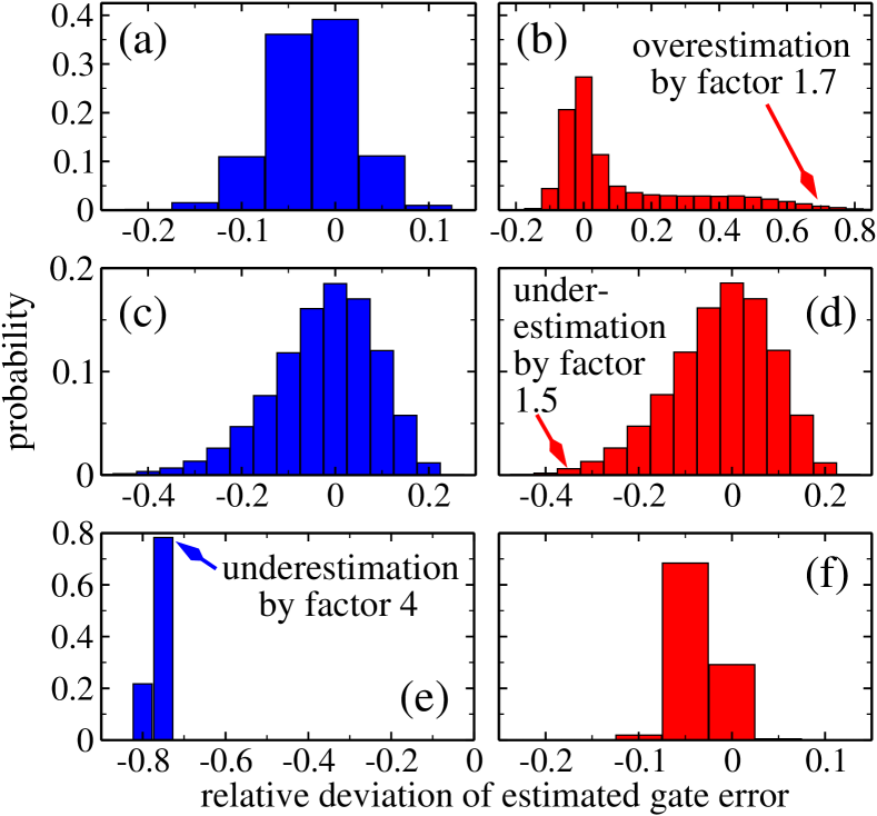
Figure 1: (Color online) Probability of the estimated gate error’s relative deviation from the standard gate error, $\Delta=(\varepsilon_{estim}-\varepsilon_{av})/\varepsilon_{av}$, for 100.000 realizations when using $F^{arith}_{unitary}$, Eq. (6), (left column) and $F^{\lambda}_{unitary}$, Eq. (8), (right column). Shown are the results for randomized dynamical maps with $O=$CNOT (a, b), truly random unitaries with $O=$CNOT (c-d) and randomized unitaries with $O=\openone$ (e-f). Positive and negative values of $\Delta$, corresponding to under- and overestimation of the gate error, do not scale equivalently. The scale for overestimation ($\Delta>0$) ranges from zero to infinity while that for underestimation ($\Delta<0$) is confined to $[-1,0)$.

Figure 1(a) shows the probability of obtaining a certain relative deviation of the estimated gate error for randomized dynamical maps and CNOT as the target gate. The randomized dynamical maps were obtained by creating a random matrix Miszczak et al. for twice as many qubits as there are system qubits. The random matrices were hermitized, multiplied by a randomly chosen scaling factor and exponentiated. The resulting matrix was multiplied by the tensor product of the target unitary with $\openone$, and the bath qubits were traced out. For most dynamical maps, $F^{arith}_{unitary}$ yields a good estimate of the gate error. If, however, the state fidelities for all $\rho_{B,i}$ are very high, but the fidelity for the totally rotated state is comparatively small, the arithmetic mean seriously underestimates the gate error. This can happen, for example, if the evolution is perfectly unitary, $\mathcal{D}(\rho_{j})=\tilde{U}\rho_{j}\tilde{U}^{+}$, and $\tilde{U}$ and the target $O$ have a common eigenbasis with all the $\rho_{B,i}$. Then the information relevant for the gate error is completely contained in $F_{TR}$. This is illustrated in Fig. 1(e) for randomized unitaries with an eigenbasis very close to the $\rho_{B,i}$ and $O=\openone$. In such a case the geometric average over all state fidelities will yield a much better estimate of the gate fidelity. In most cases, however, the geometric mean is too strict and overestimates the gate error, motivating the definition (8). Indeed, the best estimates of the gate error are obtained using $\varepsilon_{unitary}^{\lambda}=1-F^{\lambda}_{unitary}$ as shown in the right part of Fig. 1. Figure 1(a,b,e,f) presents results for randomized dynamical maps and randomized unitaries that were generated by exponentiating random Hermitian matrices. Since this is not truly random, we have also generated random unitaries based on Gram-Schmidt orthonormalization of randomly generated complex matrices Mezzadri (2007), cf. Fig. 1(c,d) with $O=$CNOT. $\varepsilon_{unitary}^{\lambda}$ yields a faithful estimate of the gate error in all cases. On average, it underestimates the gate error by factors 1.03 (Fig. 1b), 1.11 (d) and 1.02 (f) and overestimates it by 1.16 (b), 1.08 (d), and 1.01 (f). This illustrates that $F_{unitary}^{\lambda}$ makes best use of the information contained in the $d+1$ state fidelities, $F_{B,i}$ and $F_{TR}$.

$N$	type of dynamics	$\alpha^{arith}$	$\beta^{arith}$	$\alpha^{\lambda}$	$\beta^{\lambda}$
2	randomized dynamical map	0.83	1.31	0.44	1.26
	random unitaries	0.76	2.35	0.75	1.92
	randomized unitaries	1.00	4.39	0.90	1.15
3	randomized dynamical map	0.96	1.04	0.51	1.03
	random unitaries	0.90	1.32	0.90	1.32
	randomized unitaries	1.00	8.67	0.91	1.20

Table 1: Numerically obtained bounds for over- and underestimation of the average fidelity of the form $\alpha^{i}F^{i}_{unitary}\leq F_{av}\leq\beta^{i}F^{i}_{unitary}$ for the arithmetic mean over the state fidelities ($i=arith$) and the combination of arithmetic and geometric mean ($i=\lambda$), using 100.000 realizations, for 2 and 3 qubits with $O$ corresponding to CNOT ($N=2$), the Toffoli gate ($N=3$) and identity (randomized unitaries).

Bounds for over- and underestimating the gate error, obtained numerically, are presented in Table 1 with CNOT, identity and the Toffoli gate as target operations. For three-qubit gates, we find the numerical bounds to be essentially contained by those for two-qubit gates, cf. Table 1. This suggests our numerical bounds to be independent of system size. A verification of this conjecture for larger system sizes is, however, hampered by the enormous increase in numerical effort for randomization. For our examples of CNOT, the Toffoli gate and identity, we find the estimated gate error based on Eqs. (8) to deviate from the standard one in the worst case by a factor smaller than 2.5 and on average by a factor smaller than 1.2. This confirms that $d+1$ state fidelities $F_{j}$ are sufficient to accurately estimate the gate error.

III.2 Quantifying non-unitarity

If, in a given experimental setting, the gate error turns out to be larger than expected, one might want to know whether it is due to unitary errors or decoherence. This can be determined by quantifying non-unitarity of the time evolution using the following distance measure,

$$F_{diss}=1-\frac{1}{d+1}\left\{\sum_{i=1}^{d}\,\mathsf{Tr}\left[\rho^{2}_{B,i}(T)\right]+\,\mathsf{Tr}\left[\rho^{2}_{TR}(T)\right]\right\}\,,$$ (9)

where $\rho_{j}(T)=\mathcal{D}(\rho_{j})$. $F_{diss}=0$ if and only if the evolution is completely unitary. Evaluation of $F_{diss}$ requires preparation of the $d+1$ input states of Eq. (3) and measurement of $d^{2}+d$ populations.

Equation (9) cannot replace full process tomography when complete identification of the error sources is desired. However, some information can already be gained by inspection of the $d+1$ purities of Eq. (9). For example, if the purity loss is due to a single or very few terms in Eq. (9), this identifies the state evolutions that are subject to dissipation. On the other hand, if the purity loss is equally distributed over all basis states, the chosen basis is likely not an eigenbasis of the error operators (but another mutually unbiased basis presumably is).

IV Reduced set of states yielding analytical bounds on the average fidelity

We now connect our notion of a reduced set of input states to the result of Ref. Hofmann (2005) that two classical fidelities can be used to obtain an upper and a lower bound on the average fidelity. The classical fidelity is given by the average probability of obtaining the correct output for each of the $d$ classically possible input states,

$$F_{c} = \frac{1}{N}\sum_{i=1}^{d}\langle k_{i}^{\left(1\right)}|U_{0}^{\dagger}\mathcal{D}(|k_{i}^{\left(1\right)}\rangle\langle k_{i}^{\left(1\right)}|)U_{0}|k_{i}^{\left(1\right)}\rangle$$ (10)

for an arbitrary orthonormal Hilbert space basis $\{|k_{i}^{\left(1\right)}\rangle\}_{i=1,\dots,d}$. It can be interpreted as the arithmetic average over the overlaps between expected and actual population evoluation for the basis states $\ket{k_{i}^{\left(1\right)}}$. Defining $\rho_{i}^{\left(1\right)}=|k_{i}^{\left(1\right)}\rangle\langle k_{i}^{\left(1\right)}|$, such a classical fidelity can be rewritten analogously to Eq. (6),

$$F_{1} = \frac{1}{N}\sum_{i=1}^{d}\langle k_{i}^{\left(1\right)}|U_{0}\mathcal{D}\left(\rho_{i}^{\left(1\right)}\right)U_{0}^{\dagger}|k_{i}^{\left(1\right)}\rangle$$

$$= \frac{1}{N}\sum_{ij=1}^{d}\langle k_{j}^{\left(1\right)}|k_{i}^{\left(1\right)}\rangle\langle k_{i}^{\left(1\right)}|U_{0}\mathcal{D}\left(\rho_{i}^{\left(1\right)}\right)U_{0}^{\dagger}|k_{j}^{\left(1\right)}\rangle$$

$$= \frac{1}{N}\sum_{i=1}^{d}\text{Tr}\left[\rho_{i}^{\left(1\right)}U_{0}\mathcal{D}\left(\rho_{i}^{\left(1\right)}\right)U_{0}^{\dagger}\right]$$

$$= \frac{1}{N}\sum_{i=1}^{d}\text{Tr}\left[U_{0}^{\dagger}\rho_{i}^{\left(1\right)}U_{0}\mathcal{D}\left(\rho_{i}^{\left(1\right)}\right)\right]\,,$$

with $U_{0}^{\dagger}\rho_{i}^{\left(1\right)}U_{0}$ the ideal and $\mathcal{D}\left(\rho_{i}^{\left(1\right)}\right)$ the actual evolutions. In our terminology, the states $\rho_{i}^{(1)}$ ’fix’ the basis, cf. Eq. (3a). In order to fulfill the requirements of a reduced set, i.e., to allow for differentiating any two unitaries and assessing unitarity of the time evolution, another state corresponding to the totally rotated projector is necessary, cf. Section II. Instead of a single state $\rho_{TR}$, Ref. Hofmann (2005) chooses $d$ such states with each state fulfilling the condition of total rotation: $\rho_{i}^{\left(2\right)}=|k_{i}^{\left(2\right)}\rangle\langle k_{i}^{\left(2\right)}|$ with

$$\left|\Braket{k_{i}^{\left(1\right)}}{k_{j}^{\left(2\right)}}\right|^{2}=\frac{1}{d}\quad\forall i,j\,,$$

i.e., a complete mutually unbiased basis Fernández-Pérez et al. (2011). Evaluating the classical fidelities for the two bases $\{|k_{i}^{\left(1\right)}\rangle\}_{i=1,\dots,d}$, $\{|k_{i}^{\left(2\right)}\rangle\}_{i=1,\dots,d}$ then allows for analytical bounds on the average fidelity Hofmann (2005).

Note that Ref. Hofmann (2005) discusses a specific choice of the two bases. From our derivation in Section II, it is clear that any two mutually unbiased bases are suitable, and one can choose the most convenient ones. There exist $d+1=2^{N}+1$ mutually unbiased bases for $N$ qubits Wootters and Fields (1989), but only three of them consist of separable states while the remaining $d-2$ mutually unbiased bases are made up of maximally entangled states Lawrence (2011). Any two of the three separable mutually unbiased bases constitute a natural choice for most experimental setups.

V Conclusions

We have shown that a reduced set of input states can be used to estimate the average fidelity or gate error of a quantum gate. It provides the information to characterize, instead of the full open system evolution, only the unitary part. The average over all Hilbert space can then be estimated by a modified average over a reduced set of states that allows to differentiate any two unitaries and quantify non-unitarity of the evolution. The states in the reduced set correspond to a complete set of orthonormal one-dimensional projectors plus a one-dimensional projector that is rotated with respect to all the other projectors. The reduced set can be realized by two mixed states, irrespective of the dimension $d$ of the Hilbert space, or by $d+1$ pure states. Our concept of total rotation is related to the notion of mutually unbiased bases Fernández-Pérez et al. (2011) where all states of the second basis are totally rotated with respect to the first basis. It is also the underlying principle in constructing the input states for two complementary classical fidelities Hofmann (2005). Consequently, one can estimate the average fidelity using $d+1$ or $2d$ pure separable input states. In both cases, the gate error is determined in terms of state fidelities for the time-evolved states of the reduced set. The approach using $2d$ input states comes with the advantage of analytical bounds on the gate error. For the smaller set of $d+1$ input states, numerical calculations demonstrate the estimate to deviate from the true gate error by less than a factor 1.2 on average and less than a factor 2.5 in the worst case.

While the average gate fidelity currently enjoys great popularity, other very useful performance measures exist Gilchrist et al. (2005). For example, the worst case fidelity is relevant in the context of the error correction threshold Bény and Oreshkov (2010). It would be interesting to see whether the $d+1$ or $2d$ state fidelities of the reduced set allow for estimating bounds on the worst-case fidelity. This is, however, beyond the scope of our current work.

Another important question concerns the scaling of the gate error estimate employing a reduced set of states with the number of qubits. The straightforward, but not most efficient approach consists in determining the required $d+1$ or $2d$ state fidelities by state tomography. This yields a scaling of $2^{3N}$ for standard state tomography and $2^{2N}$ for Monte Carlo state characterization Flammia and Liu (2011); da Silva et al. (2011), i.e., no improvement over current approaches. Alternatively, a reduced set of states can be combined with Monte Carlo process characterization Flammia and Liu (2011); da Silva et al. (2011). We show in Ref. Reich et al. (2013) that in this case the experimental effort and the classical computational resources to obtain tight analytical bounds on the average error are reduced by a factor $2^{N}$ compared to the best currently available protocol for general unitary operations.

The ability to measure the gate performance efficiently with a reduced set of input states is not only a prerequisite for the development of quantum devices; it also opens the door to designing quantum gates in coherent control experiments using e.g. genetic algorithms where repeated checks of the performance are required.

Appendix A Proofs

We provide here detailed proofs of the claims made in Section II.

A.1 Injectivity of $\mathcal{M}$ is equivalent to the commutant space $\mathcal{K}(\{\rho_{i}\})$ having identity as its only element

Definition: Let $\rho$ be a density operator defined in a $d$-dimensional Hilbert space and $U_{i}$ elements of the projective unitary group $PU(d)$. We call the set of operators

$$K\left(\rho\right)=\left\{U_{i}\in PU(d)\,|\,\left[U_{i},\rho\right]=0\right\}$$

the commutant space of $\rho$ in $PU(d)$. The commutant space of a set of density operators $\left\{\rho_{j}\right\}$ is defined as

$$K\left(\{\rho_{j}\}\right)=\bigcap_{j}K\left(\rho_{j}\right)\,.$$

Proposition: The map $\mathcal{M}:PU(d)\to\bigoplus_{i}\mathbb{C}^{n\times n}$ which maps any unitary $U\in\text{PU$\left(d\right)$}$ to the set of propagated density operators $\left\{\rho_{i}^{(U)}\left(T\right)\right\}$ is injective iff the commutant space of $\{\rho_{i}\}$ in $PU(d)$, $\mathcal{K}(\{\rho_{i}\})$, contains only the identity.

Proof: Injectivity of $\mathcal{M}$ is equivalent to the condition

$$\forall i:\rho_{i}^{\left(U\right)}\left(T\right)=\rho_{i}^{\left(V\right)}\left(T\right)\Longleftrightarrow U=V$$

We first show that this condition is equivalent to

$$\forall i:\rho_{i}^{\left(U\right)}\left(T\right)=\rho_{i}\Longleftrightarrow U=\openone$$

Assuming validity of $\forall i:\rho_{i}^{\left(U\right)}\left(T\right)=\rho_{i}^{\left(V\right)}\left(T\right)\Longleftrightarrow U=V$ just choose $V=\openone$. Then $\rho_{i}^{\left(V\right)}\left(T\right)=\rho_{i}$ and the second statement follows immediately. Conversely, assume

$$\forall i:\rho_{i}^{\left(U\right)}\left(T\right)=\rho_{i}\Longleftrightarrow U=\openone$$

Then, for arbitrary $V,W\in PU(d)$ we set $U=V^{-1}W=V^{+}W$ and

$$\forall i:\rho_{i}^{\left(V^{+}W\right)}\left(T\right)=\rho_{i} \Longleftrightarrow \forall i:V^{+}W\rho_{i}W^{+}V=\rho_{i}$$

$$\Longleftrightarrow \forall i:W\rho_{i}W^{+}=V\rho_{i}V^{+}$$

$$\Longleftrightarrow \forall i:\rho_{i}^{\left(W\right)}\left(T\right)=\rho_{i}^{\left(V\right)}\left(T\right)$$

By assumption $\forall i:\rho_{i}^{\left(V^{+}W\right)}\left(T\right)=\rho_{i}\Longleftrightarrow V^{+}W=\openone$, but since

$$\forall i:\rho_{i}^{\left(V^{+}W\right)}\left(T\right)=\rho_{i}\Longleftrightarrow\forall i:\rho_{i}^{\left(W\right)}\left(T\right)=\rho_{i}^{\left(V\right)}\left(T\right)$$

and the relation

$$V^{+}W=\openone\Longleftrightarrow W=V$$

always holds for $V,W\in PU(d)$, this leads to the desired result: $\forall i:\rho_{i}^{\left(U\right)}\left(T\right)=\rho_{i}^{\left(V\right)}\left(T\right)\Longleftrightarrow U=V$.

We now show that $\mathcal{K}(\{\rho_{i}\})=\openone$ iff

$$\forall i:\rho_{i}^{\left(U\right)}\left(T\right)=\rho_{i}\Longleftrightarrow U=\openone$$

Consider the following calculation

$$\forall i:\rho_{i}^{\left(U\right)}\left(T\right)=\rho_{i} \Longleftrightarrow \forall i:U\rho_{i}U^{+}=\rho_{i}$$

$$\Longleftrightarrow \forall i:U\rho_{i}=\rho_{i}U$$

$$\Longleftrightarrow \forall i:U\rho_{i}-\rho_{i}U=0$$

$$\Longleftrightarrow \forall i:\left[U,\rho_{i}\right]=0$$

$$\overset{\left(*\right)}{\Longleftrightarrow} U=\openone$$

The equivalence relation $\left(*\right)$ is true only iff $\mathcal{K}(\{\rho_{i}\})=\openone$. This concludes the proof.

A.2 Total rotation and commutation with identity

Definition: Let $\mathcal{H}$ be a $d$-dimensional Hilbert space. A set $\mathcal{P}_{c}$ of $d$ one-dimensional orthogonal projectors from $\mathcal{H}$ onto itself is called complete. For example, spanning the Hilbert space by an arbitrary complete orthonormal basis $\{\ket{\varphi_{i}}|\}$, $\mathcal{P}_{c}=\{P_{i}=\ket{\varphi_{i}}\bra{\varphi_{i}}\}$. A one-dimensional projector $P_{TR}$ from $\mathcal{H}$ onto itself is called totally rotated with respect to the set $\mathcal{P}_{c}$ if $\forall P_{i}\in\mathcal{P}_{c}:\ P_{TR}P_{i}\neq 0$. A set $\mathcal{P}_{cTR}\equiv\left\{\mathcal{P}_{c},P_{TR}\right\}$ of projectors is called complete and totally rotating.

Definition: Let $\mathcal{H}$ be a $d$-dimensional Hilbert space. A set of density operators $\left\{\rho_{i}\right\}$ with $\rho_{i}\in\mathcal{H}\otimes\mathcal{H}$ is called complete if the set of projectors on the eigenspaces of the $\left\{\rho_{i}\right\}$ is complete and is called complete and totally rotating if the set of projectors on the eigenspaces of the $\left\{\rho_{i}\right\}$ is complete and totally rotating.

Our goal is to prove that the only projective unitary matrix that commutes with each element of a complete and totally rotating set of states is the identity. In order to make use of the assumed commutation relations in the proof, we translate commutation of a unitary with a state into commutation of a unitary with one or more projectors. To this end, we introduce a lemma. Using commutation of a unitary with projectors, it is then straightforward to show that the unitary must be the identity.

Lemma: If $\left[U,\rho\right]=0$ for a unitary $U\in PU(d)$ and a density operator $\rho$ which has at least one non-degenerate eigenvalue $\lambda_{1}$, then $\left[U,P_{1}\right]=0$ where $P_{1}$ is the projector onto the eigenspace $\mathcal{E}_{1}$ corresponding to the eigenvalue $\lambda_{1}$.

Proof: Since $\rho$ has a non-degenerate eigenvalue $\lambda_{1}$, we can expand it in a set of orthonormal projectors, $\rho=\lambda_{1}P_{1}+\sum_{i=2}^{d}\lambda_{i}P_{i}$, with $P_{1}=\ket{\xi_{1}}\bra{\xi_{1}}$ the projector onto the one-dimensional eigenspace $\mathcal{E}_{1}$. By assumption,

$$\left[U,\rho\right]=0 = \lambda_{1}UP_{1}-\lambda_{1}P_{1}U+\sum_{i=2}^{d}\left(\lambda_{i}UP_{i}-\lambda_{i}P_{i}U\right)$$

$$= \lambda_{1}UP_{1}U^{+}-\lambda_{1}P_{1}+\sum_{i=2}^{d}\left(\lambda_{i}UP_{i}U^{+}-\lambda_{i}P_{i}\right)\,,$$

where in the second line we have multiplied by $U^{+}$ from the right. Defining $\bar{P}_{i}=UP_{i}U^{+}$, this is equivalent to

$$\lambda_{1}\bar{P}_{1}+\sum_{i=2}^{d}\lambda_{i}\bar{P}_{i}=\lambda_{1}P_{1}+\sum_{i=2}^{d}\lambda_{i}P_{i}\,.$$

The operator equality can be applied to $\ket{\xi_{1}}$, leading to

$$\lambda_{1}\bar{P}_{1}\ket{\xi_{1}}+\sum_{i=2}^{d}\lambda_{i}\bar{P}_{i}\ket{\xi_{1}}=\lambda_{1}\ket{\xi_{1}}\,.$$

Inserting identity, $\sum_{i=1}^{d}\bar{P}_{i}=\openone$, in the right-hand side, we obtain

$$\lambda_{1}\bar{P}_{1}\ket{\xi_{1}}+\sum_{i=2}^{d}\lambda_{i}\bar{P}_{i}\ket{\xi_{1}}=\lambda_{1}\bar{P}_{1}\ket{\xi_{1}}+\sum_{i=2}^{d}\lambda_{1}\bar{P}_{i}\ket{\xi_{1}}\,.$$

Multiplying from the left by $\bar{P}_{i\neq 1}$ and using orthogonality of the $\bar{P}_{i}$ and non-degeneracy of $\lambda_{1}$, $\lambda_{i\neq 1}\neq\lambda_{1}$, we find that $\bar{P}_{i}\ket{\xi_{1}}=0$ for all $i\neq 1$. Therefore $\ket{\xi_{1}}$ lies also in the one-dimensional eigenspace corresponding to $\bar{P}_{1}$, and the one-dimensional eigenspaces of $P_{1}$ and $\bar{P}_{1}$ must be identical. This implies

$$P_{1}=\bar{P}_{1}\,,$$

and, by definition of $\bar{P}_{1}$, we find that $U$ leaves the one-dimensional eigenspace corresponding to $P_{1}$ invariant, hence commutes with $P_{1}$.

Note that if a density operator $\rho$ that commutes with $U$ has more than one non-degenerate eigenvalue, the lemma implies commutation of $U$ with all the projectors onto the one-dimensional eigenspaces.

Proposition: The only projective unitary matrix that commutes with a set of states $\{\rho_{i}\}$ that is complete and totally rotating is the identity.

Proof: Repeated application of the lemma to states $\rho_{i}$ yields a set of one-dimensional projectors that each commute with $U$. By definition of a complete and totally rotating set of states, $d+1$ projectors within this set must be elements of $\mathcal{\{}\mathcal{P}_{c},P_{TR}\}$. We can thus choose the complete set of one-dimensional projectors $\mathcal{P}_{c}$ to represent $U$, $U=\sum_{i=1}^{d}u_{i}P_{i}$. An equally valid choice $\{\tilde{P}_{i}\}$ employs the totally rotated projector, $\tilde{P}_{1}=P_{TR}$, with $\mathcal{E}_{TR}$ the corresponding eigenspace, and a suitable set of orthonormal one-dimensional projectors $\{\tilde{P}_{i}\}_{i=2,\dots,d}$ for the space $\mathcal{E}_{TR}^{\bot}$ such that $U=\sum_{i=1}^{d}u_{i}\tilde{P}_{i}$. The spectrum $\{u_{i}\}$ is of course independent of the representation. Consider the action of $U$ on a vector $\ket{\zeta}\in\mathcal{E}_{TR}$,

$$U\ket{\zeta} = \sum_{i=1}^{d}u_{i}P_{i}\ket{\zeta}$$ (11)

$$= \sum_{i=1}^{d}u_{i}\tilde{P}_{i}\ket{\zeta}=u_{1}\ket{\zeta}=\sum_{i=1}^{d}u_{1}P_{i}\ket{\zeta}\,,$$

where we have inserted $\sum_{i=1}^{d}P_{i}=\openone$ in the last step. By total rotation, $\ P_{TR}P_{i}\neq 0$ $\forall P_{i}\in\mathcal{P}_{c}$, or equivalently, $P_{i}P_{TR}\neq 0$. Applying this to $\ket{\zeta}$, we find

$$\ P_{i}P_{TR}\ket{\zeta}=P_{i}\ket{\zeta}\neq 0\quad\forall i\,.$$

Since the $P_{i}$ are one-dimensional orthonormal projectors, i.e., $P_{i}=\ket{\varphi_{i}}\bra{\varphi_{i}}$ with $\{\ket{\varphi_{i}}\}$ a complete orthonormal basis of the Hilbert space, we can rewrite $P_{i}\ket{\zeta}$,

$$P_{i}\ket{\zeta}=\mu_{i}\ket{\varphi_{i}}$$

with $\mu_{i}\in\mathbb{C}$, $\mu_{i}\neq 0$. Inserting this into Eq. (11), we obtain

$$\sum_{i=1}^{d}u_{1}\mu_{i}\ket{\varphi_{i}}=\sum_{i=1}^{d}u_{i}\mu_{i}\ket{\varphi_{i}}\,.$$

Comparing the coefficients yields $u_{1}\mu_{i}=u_{i}\mu_{i}$ $\forall i$. Since all $\mu_{i}\neq 0$ due to total rotation, we can divide and obtain

$$u_{1}=u_{i}\quad\forall i\,,$$

i.e., a unitary with complete degeneracy in its eigenvalues. This necessarily has to be the matrix $e^{i\varphi}\openone$ for $\varphi\in\left[0,2\pi\right]$, or, as an element of $PU(d)$, the unit matrix.

We have thus shown that only the identity commutes with a set of states that is complete and totally rotating. This set of states is therefore sufficient to differentiate any two unitaries.

A.3 Unitarity of $\mathcal{D}$ is equivalent to projectors being mapped onto projectors

Proposition: A dynamical map $\mathcal{D}$, defined on a $d$-dimensional Hilbert space, is unitary if and only if $\mathcal{D}$ maps (i) a set $\{P_{i}\}$ of $d$ one-dimensional orthonormal projectors onto a set of $d$ one-dimensional orthonormal projectors $\{\tilde{P}_{i}\}$ and (ii) a one-dimensional projector that is totally rotated with respect to $\{P_{i}\}$ onto a one-dimensional projector (which is totally rotated with respect to $\{\tilde{P}_{i}\}$).

Proof: We first prove the forward direction. If the time evolution is unitary, the action of $\mathcal{D}$ on any state is described by $\mathcal{D}(\rho)=U\rho U^{+}$. Specifically for orthonormal projectors $P_{i}P_{j}=\delta_{ij}$, we find

$$\mathcal{D}\left(P_{i}\right)\mathcal{D}\left(P_{j}\right)=UP_{i}U^{+}UP_{j}U^{\dagger}=UP_{i}P_{j}U^{\dagger}=\delta_{ij}UP_{i}U^{\dagger}\,.$$

Since a one-dimensional projector can be written $P_{i}=|\varphi_{i}\rangle\langle\varphi_{i}|$, where $\{\ket{\varphi_{i}}\}$ is a complete orthornormal basis of $\mathcal{H}$, $UP_{i}U^{\dagger}$ is also one-dimensional projector. By the same argument, $P_{TR}$ is mapped onto a one-dimensional projector if $\mathcal{D}(\rho)=U\rho U^{+}$. Therefore a dynamical map $\mathcal{D}$ describing unitary time evolution maps a set of $d$ orthonormal projectors, $\{P_{i}\}$, onto another such set, $\{\tilde{P}_{i}=UP_{i}U^{+}\}$, and $P_{TR}$ onto a one-dimensional projector.

We now prove the backward direction, starting from the representation of $\mathcal{D}$,

$$\mathcal{D}=\sum_{k=1}^{K}E_{k}\rho E_{k}^{+}\,,$$ (12)

by Kraus operators $E_{k}$, i.e., linear operators that fulfill

$$\sum_{k=1}^{K}E_{k}^{+}E_{k}=\openone\,.$$ (13)

We employ the canonical representation in which the Kraus operators are orthogonal, $\,\mathsf{Tr}\left[E^{+}_{k}E_{l}\right]\sim\delta_{kl}$. By assumption, a set of $d$ one-dimensional, orthonormal projectors $\{P_{i}\}$ is mapped by $\mathcal{D}$ onto another such set $\{\tilde{P}_{i}\}$,

$$\mathcal{D}\left(P_{i}\right)=\sum_{k=1}^{K}E_{k}P_{i}E_{k}^{+}=\tilde{P}_{i}\,.$$ (14)

We need to show that this implies $\mathcal{D}(\rho)=U\rho U^{+}$, or equivalently, as we demonstrate below, that $\mathcal{D}$ is made up of a single Kraus operator $E_{1}$ in the representation where $\,\mathsf{Tr}\left[E^{+}_{k}E_{l}\right]\sim\delta_{kl}$. In general, we can employ a polar decomposition for each Kraus operator, factorizing it into a unitary and a positive-semidefinite operator, $E_{k}=U_{k}\tilde{E}_{k}$. For unitary evolution, $U_{k}=\tilde{U}$ for all $k$ and $E_{1}=U\openone$ which is a special case of $\tilde{E}_{k}$ being diagonal. We first show that the assumption for the $d$ orhonormal projectors $\{P_{i}\}$ implies $U_{k}=\tilde{U}$ and diagonality of $\tilde{E}_{k}$. In a second step, we prove that the assumption for the totally rotated projector implies that there is only a single Kraus operator and $\tilde{E}_{1}=\openone$.

We first show that $\tilde{E}_{k}=E_{k}U^{+}$ is diagonal in the orthonormal basis $\{\ket{\varphi_{i}}\}$ corresponding to the $P_{i}$. Equation (14) suggests the definition of an operator $\Pi_{k}^{\left(i\right)}\equiv E_{k}P_{i}E_{k}^{+}$ which is obviously Hermitian and moreover semipositive definite. The latter is seen by making use of $P_{i}^{2}=P_{i}$ and $P_{i}=P_{i}^{+}$: $\left\langle\zeta\big{|}\Pi_{k}^{\left(i\right)}\zeta\right\rangle=\left\langle\zeta|E_{k}P_{i}P_{i}E_{k}^{+}\zeta\right\rangle=\left\langle P_{i}E_{k}^{+}\zeta|P_{i}E_{k}^{+}\zeta\right\rangle=\left\langle\xi|\xi\right\rangle\geq 0$ for any $\ket{\zeta}\in\mathcal{H}$. Equation (14) implies $\sum_{k=1}^{K}\Pi_{k}^{\left(i\right)}=\tilde{P}_{i}$. For the normalized vector spanning the eigenspace of $\tilde{P}_{i}$, $\ket{\tilde{\varphi}_{i}}\in\mathcal{E}_{i}$, we find

$$\sum_{k=1}^{K}\left\langle\tilde{\varphi}_{i}\bigg{|}\Pi_{k}^{\left(i\right)}\tilde{\varphi}_{i}\right\rangle=1\,,$$

while for all $\ket{\xi}\in\mathcal{E}_{i}^{\bot}$

$$\sum_{k=1}^{K}\left\langle\xi\bigg{|}\Pi_{k}^{\left(i\right)}\xi\right\rangle=0\,.$$

Due to positive semidefiniteness of $\Pi_{k}^{\left(i\right)}$, this implies $\left\langle\xi\big{|}\Pi_{k}^{\left(i\right)}\xi\right\rangle=0$. Reinserting the definition of $\Pi_{k}^{\left(i\right)}$ leads to $\left\langle\xi|E_{k}P_{i}E_{k}^{+}\xi\right\rangle=\left\langle P_{i}E_{k}^{+}\xi|P_{i}E_{k}^{+}\xi\right\rangle=0$, i.e., we find $P_{i}E_{k}^{+}\ket{\xi}=0$ for all $k$, $i$ and $\ket{\xi}\in\mathcal{E}_{i}^{\bot}$. For an arbitrary Hilbert space vector $\ket{\zeta}$, $\left(\openone-\tilde{P}_{i}\right)\ket{\zeta}$ lies in $\mathcal{E}_{i}^{\bot}$ such that $P_{i}E_{k}^{+}\left(\openone-\tilde{P}_{i}\right)\ket{\zeta}=0$ for all $k$ and $i$. Therefore

$$P_{i}E_{k}^{+}\left(\openone-\tilde{P}_{i}\right)=0\,,\quad\mathrm{or}\,,\quad P_{i}E_{k}^{+}=P_{i}E_{k}^{+}\tilde{P}_{i}\quad\forall i,k\,.$$

To make use of the orthogonality of the $\tilde{P}_{i}$, we multiply by $\tilde{P}_{j}$, $j\neq i$ from the right. Since $\tilde{P}_{j}$ can be written as $\tilde{P}_{j}=\tilde{U}P_{j}\tilde{U}^{+}$ for a specific $\tilde{U}$, we obtain, for all $i$, $k$ and $j\neq i$, $P_{i}E_{k}^{+}\tilde{U}P_{j}\tilde{U}^{+}=0$. Multiplication by $\tilde{U}$ from the right yields

$$P_{i}E_{k}^{+}\tilde{U}P_{j}=0\,.$$

This implies that the operators $E_{k}^{+}\tilde{U}$ have to be diagonal in the basis corresponding to the $P_{i}$,

$$E_{k}^{+}\tilde{U}=\sum_{i=1}^{d}e^{k}_{i}P_{i}\,.$$ (15)

Note that the unitary $\tilde{U}$ is the same for all Kraus operators $E_{k}$.

In the second step, we now need to show that the right-hand side of Eq. (15) is equal to the identity, making use of the assumption that the totally rotated projector is mapped by $\mathcal{D}$ onto a one-dimensional projector. The crucial information is captured in the coefficients $e^{k}_{i}$. Let us summarize what we know about the $e^{k}_{i}$. From orthogonality of the Kraus operators, we find $\,\mathsf{Tr}\left[E_{k}^{+}E_{l}\right]=\,\mathsf{Tr}\left[\sum_{i,j=1}^{d}e^{k}_{i}(e^{l}_{j})^{*}P_{i}\tilde{U}^{+}\tilde{U}P_{j}\right]=\sum_{i,j=1}^{d}e^{k}_{i}(e^{l}_{j})^{*}\,\mathsf{Tr}\left[P_{i}P_{j}\right]=\sum_{i,j=1}^{d}e^{k}_{i}(e^{l}_{j})^{*}\delta_{ij}=\sum_{i=1}^{d}e^{k}_{i}(e^{l}_{i})^{*}\overset{!}{\sim}\delta_{kl}$. The last sum can be interpreted as a scalar product for two orthogonal vectors $\vec{e}^{\;k},\vec{e}^{\;l}\in\mathbb{C}^{d}$ with coefficients $e^{k}_{i}$, $e^{l}_{i}$. Defining the proportionality constants $\mathcal{N}(k)$,

$$\mathcal{N}\left(k\right)\equiv\,\mathsf{Tr}\left[E_{k}^{+}E_{k}\right]=\sum_{i}e^{k}_{i}(e^{k}_{i})^{*}=\langle\vec{e}^{\;k},\vec{e}^{\;k}\rangle\geq 0\,,$$ (16)

we find from Eq. (13) and $\,\mathsf{Tr}[\openone]=d$ that $\sum_{k=1}^{K}\mathcal{N}(k)=d$ (and, if we can show that $\mathcal{N}(k)=d$ for one $k$, than the number of Kraus operators, $K$, must be one). Equation (13) together with Eq. (15) yields yet another condition on the $e^{k}_{i}$: $\openone=\sum_{k=1}^{K}E_{k}^{+}E_{k}=\sum_{i,j=1}^{d}\sum_{k=1}^{K}(e^{k}_{i})^{*}e^{k}_{j}P_{i}P_{j}=\sum_{i,k}\left|e^{k}_{i}\right|^{2}P_{i}$ such that $\sum_{k}\left|e^{k}_{i}\right|^{2}=1$ for each $i$. This can be interpreted as normalization condition for a vector $\vec{\epsilon}_{i}\in\mathbb{C}^{K}$ with coefficients $e^{k}_{i}$,

$$1=\sum_{k=1}^{K}\left|e^{k}_{i}\right|^{2}=\langle\vec{\epsilon}_{i},\vec{\epsilon}_{i}\rangle\,.$$ (17)

Since the vector sets $\{\vec{e}_{k}\}$ and $\{\vec{\epsilon}_{i}\}$ are not independent, it is clear that any information on the scalar product $\langle\vec{\epsilon}_{i},\vec{\epsilon}_{j}\rangle$ will be useful to determine $\mathcal{N}(k)$ (such that we can check whether there is one $k$ for which $\mathcal{N}(k)=d$). To this end, we employ the assumption that $P_{TR}$ is mapped by $\mathcal{D}$ onto a one-dimensional projector, $\tilde{P}_{TR}=\mathcal{D}(P_{TR})$, or, in other words the purity of $P_{TR}$ is preserved,

$$\,\mathsf{Tr}\left[\left(\mathcal{D}(P_{TR})\right)^{2}\right]=1\,.$$

Inserting Eqs. (12) and (15), making use of the orthogonality of the $P_{i}$ and of the trace being invariant under cyclic permutation, we find

$$\,\mathsf{Tr}\left[\mathcal{D}\left(P_{TR}\right)^{2}\right] = \,\mathsf{Tr}\left[U\left(\sum_{ij}\sum_{k}\sum_{i^{{}^{\prime}}j^{{}^{\prime}}}\sum_{k^{{}^{\prime}}}(e^{k}_{i})^{*}e^{k}_{j}(e^{k^{{}^{\prime}}}_{i^{{}^{\prime}}})^{*}e^{k^{{}^{\prime}}}_{j^{{}^{\prime}}}P_{i}P_{TR}P_{j}P_{i^{{}^{\prime}}}P_{TR}P_{j^{{}^{\prime}}}\right)U^{+}\right]$$

$$= \,\mathsf{Tr}\left[\sum_{ij}\sum_{k}\sum_{j^{{}^{\prime}}}\sum_{k^{{}^{\prime}}}(e^{k}_{i})^{*}e^{k}_{j}(e^{k^{{}^{\prime}}}_{j})^{*}e^{k^{{}^{\prime}}}_{j^{{}^{\prime}}}P_{i}P_{TR}P_{j}P_{TR}P_{j^{{}^{\prime}}}\right]$$

$$= \sum_{ij}\sum_{k}\sum_{j^{{}^{\prime}}}\sum_{k^{{}^{\prime}}}(e^{k}_{i})^{*}e^{k}_{j}(e^{k^{{}^{\prime}}}_{j})^{*}e^{k^{{}^{\prime}}}_{j^{{}^{\prime}}}\,\mathsf{Tr}\left[P_{i}P_{TR}P_{j}P_{TR}P_{j^{{}^{\prime}}}\right]$$

$$= \sum_{ij}\left|\sum_{k}(e^{k}_{i})^{*}e^{k}_{j}\right|^{2}\,\mathsf{Tr}\left[P_{i}P_{TR}P_{j}P_{TR}\right]=\sum_{ij}\left|\langle\vec{\epsilon}_{i},\vec{\epsilon}_{j}\rangle\right|^{2}\,\mathsf{Tr}\left[P_{i}P_{TR}P_{j}P_{TR}\right]\,.$$

The trace over the projectors is easily evaluated in the basis $\{\ket{\varphi_{i}}\}$, $P_{i}=\ket{\varphi_{i}}\bra{\varphi_{i}}$, in which $P_{TR}=\ket{\Psi}\bra{\Psi}$. It yields $\,\mathsf{Tr}\left[P_{i}P_{TR}P_{j}P_{TR}\right]=\left|\Braket{\varphi_{i}}{\Psi}\right|^{2}\left|\Braket{\varphi_{j}}{\Psi}\right|^{2}=\left|\mu_{i}\right|^{2}\left|\mu_{j}\right|^{2}$ with $\mu_{i}\equiv\Braket{\varphi_{i}}{\Psi}$ and $\mu_{i}\neq 0$ due to total rotation, $P_{i}P_{TR}\neq 0\forall i$. Estimating $\left|\langle\vec{\epsilon}_{i},\vec{\epsilon}_{j}\rangle\right|^{2}$ by the Cauchy Schwartz inequality, $\left|\langle\vec{\epsilon}_{i},\vec{\epsilon}_{j}\rangle\right|^{2}\leq\langle\vec{\epsilon}_{i},\vec{\epsilon}_{i}\rangle\langle\vec{\epsilon}_{j},\vec{\epsilon}_{j}\rangle$, and making use of the normalization of $\vec{\epsilon}_{i}$, cf. Eq. (17), we obtain

$$1=\,\mathsf{Tr}\left[\mathcal{D}\left(P_{TR}\right)^{2}\right] = \sum_{ij}\left|\mu_{i}\right|^{2}\left|\mu_{j}\right|^{2}\left|\langle\vec{\epsilon}_{i},\vec{\epsilon}_{j}\rangle\right|^{2}$$

$$\leq \sum_{ij}\left|\mu_{i}\right|^{2}\left|\mu_{j}\right|^{2}=1\,.$$

In the last step, we have used $\sum_{i}\left|\mu_{i}\right|^{2}=\sum_{i}\left|\Braket{\varphi_{i}}{\Psi}\right|^{2}=\sum_{i}\Braket{\Psi}{\varphi_{i}}\Braket{\varphi_{i}}{\Psi}=\Braket{\Psi}{\Psi}=1$. Since we find one on the left hand and right hand side, equality must hold for the inequality. Since $\mu_{i}\neq 0$ for all $i$, this is possible only for

$$\left|\langle\vec{\epsilon}_{i},\vec{\epsilon}_{j}\rangle\right|^{2}=1\,,\quad\mathrm{or}\,,\quad\left|\langle\vec{\epsilon}_{i},\vec{\epsilon}_{j}\rangle\right|=1\,,\quad\forall i,j\,.$$

Therefore, the normalized vectors $\vec{\epsilon}_{i}$, $\vec{\epsilon}_{j}$ are identical up to a complex scalar, $|e^{k}_{i}|=|e^{k}_{j}|$ for all $i$, $j$ and $k$. This implies for the proportionality constants $\mathcal{N}(k)$, Eq. (16), equality of all summands,

$$\mathcal{N}\left(k\right)=\sum_{i=1}^{d}e^{k}_{i}(e^{k}_{i})^{*}=d\;(e^{k}_{a})^{*}e^{k}_{a}\,.$$

Each component is thus given by $e^{k}_{i}=\sqrt{\mathcal{N}(k)/d}\exp\left[i\phi_{i}\right]$ which, making use of the orthogonality of the vectors $\vec{e}_{k}$, $\sum_{i}e^{k}_{i}(e^{l}_{i})^{*}\sim\delta_{kl}$, leads to

$$\sum_{i=1}^{d}e^{k}_{i}(e^{l}_{i})^{*} = \sum_{i=1}^{d}\frac{\sqrt{\mathcal{N}\left(k\right)\mathcal{N}\left(l\right)}}{d}\exp\left[i\phi_{i}\right]\exp\left[-i\phi_{i}\right]$$

$$= \sqrt{\mathcal{N}\left(k\right)\mathcal{N}\left(l\right)}=0\quad\forall k\neq l\,.$$

For this to be true, all $\mathcal{N}(k)$ except one and consequently all $E_{k}$ except one must be zero. By Eq. (15), its representation is

$$E=\tilde{U}\left[\sum_{i}(e^{1}_{i})^{*}P_{i}\right]\,.$$

Making use of $P_{i}P_{j}=\delta_{ij}P_{i}$ and $P_{i}=P_{i}^{+}$, unitarity of the time evolution follows immediately since

$$E^{+}E = \sum_{i=1}^{d}e^{1}_{i}(e^{1}_{i})^{*}P_{i}=\sum_{i=1}^{2}\sqrt{\frac{\mathcal{N}\left(1\right)}{d}}P_{i}=\sum_{i=1}^{k}P_{i}=\openone\,,$$

$$EE^{+} = \tilde{U}\left(\sum_{i=1}e^{1}_{i}(e^{1}_{i})^{*}P_{i}\right)\tilde{U}^{+}=\tilde{U}\openone\tilde{U}^{+}=\openone\,,$$

such that

$$\mathcal{D}\left(\rho\right)=\tilde{U}\rho\tilde{U}^{+}$$

for a unitary $\tilde{U}\in\text{PU$\left(d\right)$}$. This concludes the proof.

References

• Nielsen and Chuang (2000) M. A. Nielsen and I. L. Chuang, Quantum Computation and Quantum Information (Cambridge University Press, 2000).
• Mohseni et al. (2008) M. Mohseni, A. T. Rezakhani, and D. A. Lidar, Phys. Rev. A 77, 032322 (2008).
• Flammia and Liu (2011) S. T. Flammia and Y.-K. Liu, Phys. Rev. Lett. 106, 230501 (2011).
• da Silva et al. (2011) M. P. da Silva, O. Landon-Cardinal, and D. Poulin, Phys. Rev. Lett. 107, 210404 (2011).
• Shabani et al. (2011) A. Shabani, R. L. Kosut, M. Mohseni, H. Rabitz, M. A. Broome, M. P. Almeida, A. Fedrizzi, and A. G. White, Phys. Rev. Lett. 106, 100401 (2011).
• Schmiegelow et al. (2011) C. T. Schmiegelow, A. Bendersky, M. A. Larotonda, and J. P. Paz, Phys. Rev. Lett. 107, 100502 (2011).
• Mohseni and Rezakhani (2009) M. Mohseni and A. T. Rezakhani, Phys. Rev. A 80, 010101 (2009).
• Steffen et al. (2012) L. Steffen, M. P. da Silva, A. Fedorov, M. Baur, and A. Wallraff, Phys. Rev. Lett. 108, 260506 (2012).
• Bendersky et al. (2008) A. Bendersky, F. Pastawski, and J. P. Paz, Phys. Rev. Lett. 100, 190403 (2008).
• Lawrence (2011) J. Lawrence, Phys. Rev. A 84, 022338 (2011).
• Hofmann (2005) H. F. Hofmann, Phys. Rev. Lett. 94, 160504 (2005).
• Lanyon et al. (2011) B. P. Lanyon, C. Hempel, D. Nigg, M. Müller, R. Gerritsma, F. Zähringer, P. Schindler, J. T. Barreiro, M. Rambach, G. Kirchmair, et al., Science 334, 57 (2011).
• Kallush and Kosloff (2006) S. Kallush and R. Kosloff, Phys. Rev. A 73, 032324 (2006).
• (14) J. A. Miszczak, Z. Puchała, and P. Gawron, Quantum Information package for Mathematica, http://zksi.iitis.pl/wiki/projects:mathematica-qi.
• Mezzadri (2007) F. Mezzadri, Notices of the AMS 54, 592 (2007).
• Fernández-Pérez et al. (2011) A. Fernández-Pérez, A. B. Klimov, and C. Saavedra, Phys. Rev. A 83, 052332 (2011).
• Wootters and Fields (1989) W. K. Wootters and B. D. Fields, Ann. Phys. 191, 363 (1989).
• Gilchrist et al. (2005) A. Gilchrist, N. K. Langford, and M. A. Nielsen, Phys. Rev. A 71, 062310 (2005).
• Bény and Oreshkov (2010) C. Bény and O. Oreshkov, Phys. Rev. Lett. 104, 120501 (2010).
• Reich et al. (2013) D. M. Reich, G. Gualdi, and C. P. Koch, arXiv:1305.5649 (2013).