Empirical Analysis of Stochastic Volatility Model by Hybrid Monte Carlo Algorithm

Abstract

The stochastic volatility model is one of volatility models which infer latent volatility of asset returns. The Bayesian inference of the stochastic volatility (SV) model is performed by the hybrid Monte Carlo (HMC) algorithm which is superior to other Markov Chain Monte Carlo methods in sampling volatility variables. We perform the HMC simulations of the SV model for two liquid stock returns traded on the Tokyo Stock Exchange and measure the volatilities of those stock returns. Then we calculate the accuracy of the volatility measurement using the realized volatility as a proxy of the true volatility and compare the SV model with the GARCH model which is one of other volatility models. Using the accuracy calculated with the realized volatility we find that empirically the SV model performs better than the GARCH model.

1 Introduction

Statistical properties of asset price returns have been extensively studied both in finance and econophysics. It is well-known that asset price returns show fat-tailed distributions and volatility clustering which are now classified as stylized facts[1, 2]. Although in empirical finance the volatility is an important value to measure the risk it is quite difficult to extract the true volatility from asset price returns themselves. A popular technique to measure the volatility is to use volatility models which mimic volatility properties of asset returns such as volatility clustering. A famous volatility model is the generalized autoregressive conditional hetroskedasticity (GARCH) model[3, 4] where the volatility variable changes deterministically depending on the past squared value of the returns and past volatilities. There exist many extended versions of GARCH models, such as EGARCH[5], GJR[6], QGARCH[7, 8], GARCH-RE[9] models and many others, e.g. [10, 11], which are designed to increase the performance of the model.

The stochastic volatility (SV) model[12, 13] is another model which captures the properties of the volatility. Unlike the GARCH model, the volatility of the SV model changes stochastically in time. As a result the likelihood function of the SV model is given as a multiple integral of the volatility variables. Such an integral in general is not analytically calculable and thus the determination of the parameters of the SV model by the maximum likelihood method becomes extremely difficult. To overcome this difficulty the Markov Chain Monte Carlo (MCMC) method based on the Bayesian approach is proposed and developed[12]. In the MCMC method of the SV model one has to update not only the parameter variables but also the volatility ones under a joint probability distribution of the model parameters and the volatility variables. Although there exist various MCMC methods to perform the Bayesian program the performance of the MCMC technique depends on each MCMC method. A local update scheme is usually not effective for the SV model which has an increasing number of volatility variables with the data size of return time series[14]. In order to improve the efficiency of the local update method the blocked scheme which updates several variables simultaneously is proposed[14, 15].

In this study we use the HMC algorithm[16] which is a global algorithm updating variables simultaneously. This global property of the HMC algorithm could be advantageous for updating volatility variables of the SV model. Actually it is shown that the HMC algorithm can decorrelate first enough the sampled data of the volatility variables[17, 18]. The HMC has been also applied to the parameter estimation of the GARCH model[19].

Using the HMC algorithm we perform the Bayesian inference of the SV model for two stock returns (Mitsubishi Co. and Panasonic Co.) traded on the Tokyo Stock Exchange and measure the volatility of those stock returns. In order to quantify the accuracy of the volatility estimated from the SV model we calculate a loss function using the realized volatility from the high-frequency intraday returns as a proxy of the true volatility. The realized volatility as a proxy of the true volatility has been used for ranking GARCH-type models[20]. In this study we also calculate the accuracy of the volatility from the GARCH model and compare the SV model and the GARCH model based on the criterion of the volatility accuracy.

2 Stochastic Volatility Model

The standard SV model[12, 13] is defined by

$$y_{t}=\sigma_{t}\epsilon_{t}=\exp(h_{t}/2)\epsilon_{t},$$ (1)

$$h_{t}=\mu+\phi(h_{t-1}-\mu)+\eta_{t},$$ (2)

where $h_{t}$ is defined by $h_{t}=\ln\sigma_{t}^{2}$, and $\sigma_{t}$ is called volatility. We also call $h_{t}$ volatility variable. The error terms $\epsilon_{t}$ and $\eta_{t}$ are taken from independent normal distributions $N(0,1)$ and $N(0,\sigma_{\eta}^{2})$ respectively.

This model contains three parameters $\mu$, $\phi$ and $\sigma^{2}_{\eta}$ which have to be inferred so that the model could match the asset return data $y_{t}$ measured in the financial markets. Let $\theta$ be an abbreviation for $\mu$, $\phi$ and $\sigma^{2}_{\eta}$, i.e. $\theta=(\mu,\phi,\sigma^{2}_{\eta})$. Then the likelihood function $L({\bf\theta})$ of the SV model can be written as

$$L({\bf\theta})=\int\prod_{t=1}^{n}f(\epsilon_{t}|\sigma_{t}^{2})f(h_{t}|\theta)dh_{1}dh_{2}...dh_{n},$$ (3)

where

$$f(\epsilon_{t}|\sigma_{t}^{2})=\left(2\pi\sigma_{t}^{2}\right)^{-\frac{1}{2}}\exp\left(-\frac{y_{t}^{2}}{2\sigma_{t}^{2}}\right),$$ (4)

$$f(h_{1}|\theta)=\left(\frac{2\pi\sigma_{\eta}^{2}}{1-\phi^{2}}\right)^{-\frac{1}{2}}\exp\left(-\frac{[h_{1}-\mu]^{2}}{2\sigma_{\eta}^{2}/(1-\phi^{2})}\right),$$ (5)

$$f(h_{t}|\theta)=\left(2\pi\sigma_{\eta}^{2}\right)^{-\frac{1}{2}}\exp\left(-\frac{[h_{t}-\mu-\phi(h_{t-1}-\mu)]^{2}}{2\sigma_{\eta}^{2}}\right).$$ (6)

Unlike the GARCH model where the maximum likelihood method should work, $L({\bf\theta})$ of the SV model is constructed as a multiple integral of the volatility variables which makes the maximum likelihood estimation difficult. A possible estimation technique for the SV model is the Bayesian inference performed by the MCMC method. In the Bayesian inference model parameters are inferred as the expectation values given by

$$\langle{\bf\theta_{i}}\rangle=\int{\bf\theta_{i}}f(\theta|y)\Pi_{k=1}^{3}d\theta_{k},$$ (7)

where $(\theta_{1},\theta_{2},\theta_{3})=(\mu,\phi,\sigma^{2}_{\eta})$ and $f(\theta|y)$ is the probability distribution of $\theta$ constructed by the likelihood function and the prior distribution of $\pi(\theta)$ as

$$f(\theta|y)\sim L({\bf\theta})\pi(\bf\theta).$$ (8)

In general eq.(7) can not be performed analytically and usually it is estimated numerically by the MCMC method. Since $L(\theta)$ also contains the integral of volatility variables $h_{t}$ we have to update not only the model parameter $\theta$ but also the volatility variables $h_{t}$ in the MCMC method. To update the model parameter $\theta$ we follow the standard update technique[12, 13].

The probability distribution of the volatility variables $h_{t}$ is given by

$$P(h_{t})\equiv P(h_{1},h_{2},...,h_{n})\sim\vspace{2cm}$$ (9)

$$\exp\left(-\sum_{i=1}^{n}\{\frac{h_{i}}{2}+\frac{\epsilon_{i}^{2}}{2}e^{-h_{i}}\}-\frac{[h_{1}-\mu]^{2}}{2\sigma_{\eta}^{2}/(1-\phi^{2})}-\sum_{i=2}^{n}\frac{[h_{i}-\mu-\phi(h_{i-1}-\mu)]^{2}}{2\sigma_{\eta}^{2}}\right).$$

To update the volatility variables with this probability distribution we use the HMC algorithm.

3 Hybrid Monte Carlo Algorithm

The HMC algorithm is a global MCMC one which can update simultaneously all the variables of the model we consider. Originally the HMC algorithm is developed for the MCMC simulations of the lattice Quantum Chromo Dynamics (QCD) calculations[16, 21] where a very large scale simulation with a huge number of variables is inevitable. The basic idea of the HMC algorithm is a combination of molecular dynamics (MD) simulation and Metropolis accept/reject step. In the HMC algorithm we first introduce momentum variables $p_{i}$ conjugate to $h_{i}$ and define the Hamiltonian of the SV model[17, 18] as

$$H(p_{t},h_{t})=\sum_{i=1}^{n}\frac{1}{2}p_{i}^{2}+\sum_{i=1}^{n}\{\frac{h_{i}}{2}+\frac{\epsilon_{i}^{2}}{2}e^{-h_{i}}\}+\frac{[h_{1}-\mu]^{2}}{2\sigma_{\eta}^{2}/(1-\phi^{2})}+\sum_{i=2}^{n}\frac{[h_{i}-\mu-\phi(h_{i-1}-\mu)]^{2}}{2\sigma_{\eta}^{2}}.$$ (10)

Then we integrate the Hamilton’s equations of motion,

$$\frac{\displaystyle dh_{i}}{\displaystyle d\tau}= \frac{\partial H}{\partial p_{i}},$$ (11)

$$\frac{\displaystyle dp_{i}}{\displaystyle d\tau}= -\frac{\partial H}{\partial h_{i}},$$ (12)

numerically by doing the MD simulation in the fictitious time $\tau$. The simplest integrator for the MD simulation is the 2nd order leapfrog integrator[16] given by

$$h_{i}(\tau+\Delta\tau/2) =h_{i}(\tau)+\frac{\Delta\tau}{2}p_{i}(\tau)$$ (13)

$$p_{i}(\tau+\Delta\tau) =p_{i}(\tau)-\Delta\tau\frac{\partial H(p_{t},h_{t})}{\partial h_{i}}$$

$$h_{i}(\tau+\Delta\tau) =h_{i}(\tau+\Delta\tau/2)+\frac{\Delta\tau}{2}p_{i}(\tau+\Delta\tau),$$

where $\Delta\tau$ is a step size of the MC simulation. Although we adopt this 2nd order leapfrog integrator in this study we could also use the other improved integrators[22] or higher order integrators[23, 24].

After integrating the Hamilton’s equations of motion up to some constant time, we obtain a set of new candidate variables $(p^{\prime},h^{\prime})$. These candidates are accepted with the Metropolis test[25] with the following probability,

$$P=\min\{1,\frac{\exp\left(-H(p^{\prime},h^{\prime})\right)}{\exp\left(-H(p,h)\right)}\}=\min\{1,\exp\left(-\Delta H\right)\},$$ (14)

where $\Delta H$ is the energy difference given by $\Delta H=H(p^{\prime},h^{\prime})-H(p,h)$. The acceptance rate of eq.(14) can be tuned by $\Delta\tau$. The high acceptance rate is not necessary for the HMC and it is shown that the optimum acceptance rate of the HMC with the 2nd order integrator is around 60%[23].

4 Realized Volatility

In this study we use the realized volatility as a proxy of the true volatility and use it for the accuracy calculation of the volatility inferred from the volatility models. When high-frequency intraday return data is available we can construct the realized volatility as a sum of squared intraday returns[26, 27, 28]. Let us assume that the logarithmic price process $\ln p(s)$ follows a continuous time stochastic diffusion,

$$d\ln p(s)=\tilde{\sigma}(s)dW(s),$$ (15)

where $W(s)$ stands for a standard Brownian motion and $\tilde{\sigma}(s)$ is a spot volatility at time $s$. Then the integrated volatility is defined by

$$\sigma_{T}^{2}(t)=\int_{t}^{t+T}\tilde{\sigma}(s)^{2}ds,$$ (16)

where $T$ stands for the interval to be integrated. If we consider daily volatility $T$ should take one day. Since $\tilde{\sigma}(s)$ is latent and not available from market data, the value of eq.(16) can not be obtained directly.

Constructing $n$ intraday returns from high-frequency data, the realized volatility $RV_{t}$ is given by a sum of squared intraday returns,

$$RV_{t}=\sum_{i=1}^{n}r_{t+i\delta}^{2},$$ (17)

where $\delta$ is a sampling time interval defined by $\delta=T/n$. Note that small sampling time interval corresponds to high sampling frequency.

If there is no microstructure noise[29, 30], $RV_{t}$ goes to the integrated volatility of eq.(16) in the limit of $n\rightarrow\infty$. Empirically it is well-known that the realized volatility measure suffers from the microstructure noise and the distortion from the microstructure noise will be serious at very high-frequency. Such distortion can be depicted in the volatility signature plot[31]. To avoid a large distortion on the realized volatility and at the same time to maintain the accuracy of the realized volatility measure we have to employ a good sampling frequency. The optimum sampling frequency under the independent microstructure noise was derived and found to be between one and five minutes[32]

When we consider daily stock realized volatility we have to cope with non-trading hours issue. Usually high-frequency data are not available for the entire 24 hours. At the Tokyo stock exchange market domestic stocks are traded in the two trading sessions: (1)morning trading session (MS) 9:00-11:00. (2)afternoon trading session (AS) 12:30-15:00. The daily realized volatility calculated without including intraday returns during the non-traded periods can be underestimated.

An idea to circumvent the problem is advocated by Hansen and Lunde[33]. They introduced an adjustment factor which modifies the realized volatility so that the average of the realized volatility matches the variance of the daily returns. Let $(R_{1},...,R_{N})$ be $N$ daily returns. The adjustment factor $c$ is given by

$$c=\frac{\sum_{t=1}^{N}(R_{t}-\bar{R})^{2}}{\sum_{t=1}^{N}RV_{t}},$$ (18)

where $\bar{R}$ denotes the average of $R_{t}$. Here we call $c$ the HL factor. Then using this factor the daily realized volatility is modified to $cRV_{t}$. In this study we calculate the realized volatility and the HL factor at several sampling frequencies and use the modified realized volatility $cRV_{t}$ as a proxy of the true daily volatility.

Table 1: Results estimated by the HMC algorithm. SD stands for Standard Deviation and SE stands for Statistical Error. The statistical errors are estimated by the jackknife method. $\tau_{int}$ is the autocorrelation time defined by $\tau_{int}=1+2\sum_{t=1}^{\infty}ACF(t)$, where $ACF(t)$ is the autocorrelation function. We also show $h_{10}$ as a representative one of the volatility variables $h_{t}$.

		$\phi$	$\mu$	$\sigma^{2}_{\eta}$	$h_{10}$
Mitsubishi Co.		0.987	-7.33	0.0186	-7.48
	SD	0.007	1.07	0.067	0.31
	SE	0.0005	0.007	0.0008	0.01
	$\tau_{int}$	260(130)	1.3(1)	800(370)	30(4)
Panasonic Co.		0.975	-7.87	0.045	-7.57
	SD	0.012	0.50	0.017	0.36
	SE	0.0013	0.004	0.0025	0.01
	$\tau_{int}$	410(250)	1.8(4)	800(480)	35(14)

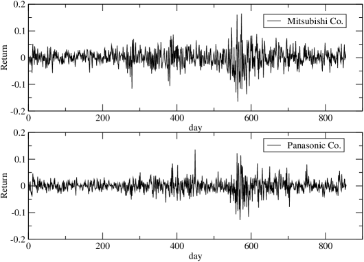
Figure 1: Daily close-to-close return time series of Mitsubishi Co. (top) and Panasonic Co. (bottom).

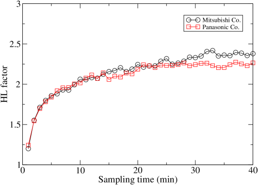
Figure 2: HL factor as a function of sampling time interval.

5 Empirical Analysis

In this section we empirically study the SV model by applying it for asset returns traded on the Tokyo Stock Exchange. The empirical study is based on daily data of two stocks (Mitsubishi Co. and Panasonic Co.). These stocks are included in the list of the Topix core 30 index which collects liquid stocks of the Tokyo Stock Exchange. The sampling period of the stock data is June 3, 1996 to December 30, 2009. Figure 1 shows the daily close-to-close returns of the two stocks.

Using the daily close-to-close return data of Mitsubishi Co. and Panasonic Co. we perform the Bayesian inference by the MCMC method for the SV model. The first 10000 Monte Carlo samples are discarded and then 40000 samples are recorded for the analysis. The MCMC sampling of the volatility variables is performed by the HMC method. The MCMC sampling of the model parameters $(\mu,\phi,\sigma^{2}_{\eta})$ is implemented by the standard MCMC method[13]. The values of the model parameters obtained by the MCMC method are summarized in table 1. We also list the results of $h_{10}$ in the table as a representative one of volatility variables. It is found that the autocorrelation time of $h_{10}$ is not big but around 30 which is much smaller than that of the Metropolis algorithm[18].

We measure the accuracy of the volatility from the SV model by calculating the following loss function.

$$RMSPE=\sqrt{\frac{1}{N}\sum_{t=1}^{N}\left(\frac{{\bar{\sigma}_{t}^{2}}-cRV_{t}}{cRV_{t}}\right)^{2}},$$ (19)

where RMSPE stands for the Root Mean Squared Percentage Error and $\bar{\sigma}_{t}^{2}$ is a volatility value at time $t$ averaged over the volatility data sampled by the HMC.

The realized volatility is calculated using sampling time from 1-min. to 20-min. For each sampling time we also calculate the HL factor of eq.(18). Figure 2 shows the HL factors of Mitsubishi Co. and Panasonic Co as a function of sampling time interval. We find that both the HL factors from two stocks behave similarly and increase with sampling time interval. The smaller HL factors at small sampling time interval, i.e. at high sampling frequency are caused by the microstructure noise which artificially inflates the realized volatility. At bigger sampling time interval, i.e. at lower sampling frequency where the microstructure noise effect is negligible the HL factors take bigger than 2, which means that returns during non-trading hours moves as much as returns during trading hours. Especially it is found that overnight return change dominates in non-trading hours[34].

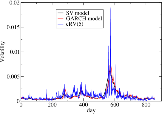
Figure 3: Volatility of Mitsubishi Co. obtained from the SV model, the GARCH model and the realized volatility ($cRV(5)$) at 5-min sampling frequency.

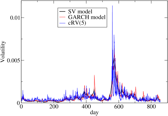
Figure 4: Volatility of Panasonic Co. obtained from the SV model, the GARCH model and the realized volatility ($cRV(5)$) at 5-min sampling frequency.

Using the HL factor $c$ we scale the realized volatility $RV_{t}$ to $cRV_{t}$. Figure 3-4 compare the scaled realized volatility $cRV_{t}$ and the volatility from the SV model. In the figures we only show the realized volatility constructed at 5-min sampling frequency as a representative one. The volatility estimated from the GARCH model is also shown in the figures. We used the GARCH(1,1) model with normal errors which is commonly used in empirical analysis of asset volatility. The MCMC method[35, 36, 37, 38] was also used for the volatility estimation of the GARCH model.

Figure 5 shows the RMSPE of the SV and the GARCH model. It is seen that the RMSPE of the SV model is smaller than that of the GARCH model which indicates that the SV model is superior to the GARCH model. It is also interesting to notice that the minimum of the RMSPE takes around 5-min and this observation is consistent with the optimum sampling time interval suggested in [32].

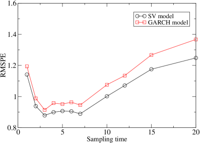
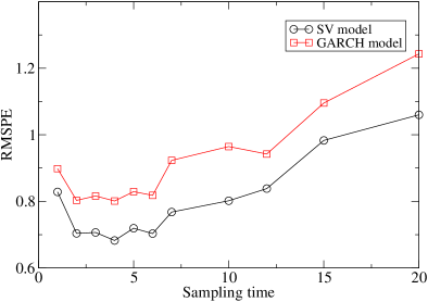
Figure 5: RMSPE of the SV model and the GARCH model for Mitsubishi Co. (left) and Panasonic Co. (right).

6 Conclusions

We applied the HMC algorithm to the Bayesian inference of the SV model and estimated the volatility of two stock returns (Mitsubishi Co. and Panasonic Co.) traded on the Tokyo Stock Exchange. We find that the volatility variables sampled by the HMC algorithm are well decorrelated compared to the Metopolis algorithm. In order to quantify the accuracy of the estimated volatility we calculated the RMSPE using the realized volatility modified by the HL factor as a proxy of the true volatility. Comparing the RMSPE of the SV model with that of the GARCH model we find that the volatility accuracy of the SV model is superior to that of the GARCH model. Therefore empirically the SV model is preferred to the GARCH model based on the criterion of the volatility accuracy.

Since in this study we only used the GARCH(1,1) model it might be interesting further to compare the SV model with other relevant GARCH-type models.

Acknowledgments.

Numerical calculations in this work were carried out at the Yukawa Institute Computer Facility and the facilities of the Institute of Statistical Mathematics. This work was supported by Grant-in-Aid for Scientific Research (C) (No.22500267).

References

References

- [1] Mantegna R and Stanley H E, Introduction to Econophysics (Cambridge University Press, 1999).
- [2] Cont R 2001 Empirical Properties of Asset Returns: Stylized Facts and Statistical Issues Quantitative Finance 1 223–236
- [3] Engle R.R 1982 Autoregressive Conditional Heteroskedasticity with Estimates of the Variance of the United Kingdom inflation Econometrica 60 987–1007
- [4] Bollerslev T 1986 Generalized Autoregressive Conditional Heteroskedasticity Journal of Econometrics 31 307–327.
- [5] Nelson D B 1991 Conditional Heteroskedasticity in Asset Returns: A New Approach Econometrica 59 347–370
- [6] Glosten L R, Jaganathan R and Runkle D E 1993 On the Relation Between the Expected Value and the Volatility of the Nominal Excess on Stocks Journal of Finance 48 1779–1801
- [7] Engle R F and Ng V 1993 Measuring and Testing the Impact of News on Volatility Journal of Finance 48 1749–1778
- [8] Sentana E 1995 Quadratic ARCH models Review of Economic Studies 62 639–661
- [9] Takasihi T and Chen T T 2012 Bayesian Inference of the GARCH model with Rational Errors International Proceedings of Economics Development and Research 29 303–307
- [10] Bollerslev T, Chou R Y and Kroner K F 1992 ARCH modeling in finance Journal of Econometrics 52 5–59
- [11] Xekalaki E and Degiannakis S 2010 ARCH Models for Financial Applications ( John Wiley & Sons Ltd. )
- [12] Jacquier E, Polson N G and Rossi P E 1994 Bayesian Analysis of Stochastic Volatility Models Journal of Business & Economic Statistics 12 371–389
- [13] Kim S, Shephard N and Chib S 1998 Stochastic Volatility: Likelihood Inference and Comparison with ARCH Models Review of Economic Studies 65 361–393.
- [14] Shephard N and Pitt M K 1997 Likelihood Analysis of Non-Gaussian Measurement Time Series Biometrika 84 653–667
- [15] Watanabe T and Omori Y 2004 A Multi-move Sampler for Estimating Non-Gaussian Time Series Models Biometrika 91 246–248
- [16] Duane S, Kennedy A D, Pendleton B J and Roweth D 1987 Hybrid Monte Carlo Phys. Lett. B 195 216–222
- [17] Takaishi T 2008 Financial Time Series Analysis of SV Model by Hybrid Monte Carlo Lecture Notes in Computer Science 5226 929–936
- [18] Takasihi T 2009 Bayesian Inference of Stochastic Volatility Model by Hybrid Monte Carlo Journal of Circuits, Systems, and Computers 18 1381–1396
-
[19]
Takaishi T 2006 Bayesian estimation of GARCH model by Hybrid Monte Carlo
Proceedings of the 9th Joint Conference on Information Sciences 2006, CIEF-214
doi:10.2991/jcis.2006.159 - [20] Hansen P R and Lunde A 2006 Consistent ranking of volatility models Journal of Econometrics 131 97–121
- [21] Ukawa A 1989 Lattice QCD Simulations Beyond the Quenched Approximation Nucl. Phys. B (Proc. Suppl.) 10 66–145
- [22] Takaishi T and de Forcrand Ph 2008 Testing and Tuning Symplectic Integrators for Hybrid Monte Carlo Algorithm in Lattice QCD Phys. Rev. E 73 036706
- [23] Takaishi T 2000 Choice of Integrators in the Hybrid Monte Carlo Algorithm Comput. Phys. Commun. 133 6–17
- [24] Takaishi T 2002 Higher Order Hybrid Monte Carlo at Finite Temperature Phys. Lett. B 540 159–165
- [25] Metropolis N, Rosenbluth A W, Rosenbluth M N, Teller A H and Teller E 1953 Equations of State Calculations by Fast Computing Machines J. of Chem. Phys. 21 1087–1091
- [26] Andersen T G and Bollerslev T 1998 Answering the Skeptics: Yes, Standard Volatility Models do Provide Accurate Forecasts International Economic Review 39 885–905
- [27] Andersen T G, Bollerslev T, Diebold F X and Labys P 2001 The distribution of realized exchange rate volatility Journal of the American Statistical Association 96 42–55
- [28] Andersen T G, Bollerslev T, Diebold F X and Ebens H 2001 The distribution of realized stock return volatility Journal of Financial Economics 61 43–76
- [29] Campbell J Y, Lo A W and MacKinlay A C 1997 The Econometrics of Financial Markets ( Princeton University Press )
- [30] Zhou B 1996 High-frequency data and volatility in foreign-exchange rates Journal of Business & Economics Statistics 14 45–52
- [31] Andersen T G, Bollerslev T, Diebold F X and Labys P 2000 Great Realization Risk, March 105–108
- [32] Bandi F M and Russell J R 2008 “ Microstructure noise, realized variance, and optimal sampling The Review of Economic Studies 75 339-369
- [33] Hansen P R and Lunde A 2005 A forecast comparison of volatility models: does anything beat a GARCH(1,1)? Journal of Applied Econometrics 20 873-889
- [34] Takaishi T, Chen T T and Zheng Z 2012 Analysis of Realized Volatility in Two Trading Sessions of the Japanese Stock Market Prog. Theor. Phys. Supplement 194 43-54
- [35] Takaishi T 2009 An Adaptive Markov Chain Monte Carlo Method for GARCH Model Lecture Notes of the Institute for Computer Sciences, Social Informatics and Telecommunications Engineering. Complex Sciences Vol. 5 1424
- [36] Takaishi T 2009 Bayesian Estimation of GARCH Model with an Adaptive Proposal Density New Advances in Intelligent Decision Technologies, Studies in Computational Intelligence Vol. 199 635
- [37] Takaishi T 2009 Bayesian Inference on QGARCH Model Using the Adaptive Construction Scheme Proceedings of 8th IEEE/ACIS International Conference on Computer and Information Science 525–529 doi:10.1109/ICIS.2009.173
- [38] Takaishi T 2010 Bayesian inference with an adaptive proposal density for GARCH models J. Phys.: Conf. Ser. 221 012011