¹¹institutetext: INAF - Osservatorio Astrofisico di Arcetri, Largo E. Fermi 5, I-50125, Firenze, Italy ¹¹email: oliva@arcetri.inaf.it ²²institutetext: INAF - Osservatorio Astronomico di Bologna, via Ranzani 1, I-40127 Bologna, Italy ³³institutetext: Cavendish Laboratory, University of Cambridge, 19 J. J. Thomson Avenue, Cambridge CB3 0HE, UK ⁴⁴institutetext: INAF - Osservatorio Astrofisico di Catania, via S. Sofia 78, I-95123 Catania, Italy ⁵⁵institutetext: INAF - Fundación Galileo Galilei, Rambla José Ana Fernández Pérez, 7, 38712 Breña Baja, TF, Spain ⁶⁶institutetext: Dipartimento di Fisica e Astronomia, Sezione Astrofisica, Università di Catania, via S. Sofia 78, I-95123 Catania, Italy ⁷⁷institutetext: Lawrence Berkeley National Laboratory, MS 2-400, One Cyclotron Road, Berkeley, CA 94720, USA ⁸⁸institutetext: Dipartimento di Astronomia, Università di Bologna, Via Ranzani 1, I-40127 Bologna, Italy ⁹⁹institutetext: European Southern Observatory, Karl-Schwarzschild-Str. 2, D-85748 Garching bei Muenchen, Germany

A GIANO-TNG high resolution IR spectrum of the airglow emission

E. Oliva 11 L. Origlia 22 R. Maiolino 33 C. Baffa 11 V. Biliotti 11 P. Bruno 44 G. Falcini 11 V. Gavriousev 11 F. Ghinassi 55 E. Giani 11 M. Gonzalez 55 F. Leone 66 M. Lodi 55 F. Massi 11 P. Montegriffo 22 I. Mochi 77 M. Pedani 55 E. Rossetti 88 S. Scuderi 55 M. Sozzi 11 A. Tozzi 11 E. Valenti 99

(Received …. ; accepted …)

Abstract

Aims. A flux-calibrated high resolution spectrum of the airglow emission is a practical $\lambda$ -calibration reference for astronomical spectral observations. It is also useful for constraining the molecular parameters of the OH molecule and the physical conditions in the upper mesosphere.

Methods. We use the data collected during the first technical commissioning of the GIANO spectrograph at the Telescopio Nazionale Galileo (TNG). The high resolution (R $\simeq$ 50,000) spectrum simultaneously covers the 0.95-2.4 $\mu$ m wavelength range. Relative flux calibration is achieved by the simultaneous observation of a spectrophotometric standard star.

Results. We derive a list of improved positions and intensities of OH infrared lines. The list includes $\Lambda$ -split doublets many of which are spectrally resolved. Compared to previous works, the new results correct errors in the wavelengths of the Q-branch transitions. The relative fluxes of OH lines from different vibrational bands show remarkable deviations from theoretical predictions: the $\Delta v$ =3,4 lines are a factor of 2 and 4 brighter than expected. We also find evidence of a significant fraction (1-4%) of OH molecules with “non-thermal” population of high-J levels. Finally we list wavelengths and fluxes of 153 lines not attributable to OH. Most of these can be associated to O₂, while 37 lines in the H band are not identified. The O₂ and unidentified lines in the H band account for $\simeq$ 5% of the total airglow flux in this band.

Key Words.:

Line: identification – Infrared: general – Techniques: spectroscopic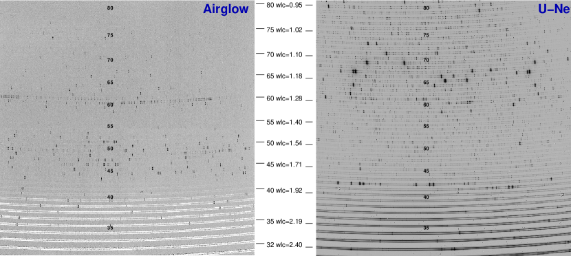

Refer to caption — Figure 1: GIANO echelle spectra of the airglow emission (left panel) and of the U-Ne calibration lamp (right-hand panel). The positions of several orders and the corresponding central wavelengths (in $\mu$ m) are marked.

1 Introduction

The airglow emission is an annoying, unavoidable contamination of all ground-based astronomical observations. It mostly consists of narrow lines of molecular bands which, on the other hand, could be conveniently used as a reference spectrum for wavelength calibration of spectroscopic data. The airglow lines at wavelengths 0.3–1.0 $\mu$ m have been thoroughly compiled and modelled using high resolution (R $\simeq$ 10⁵) data from HIRES-Keck and UVES-VLT; see e.g. Osterbrock et al. Osterbrock98 (1998), Hanuschik Hanushik (2003), Cosby et al. Cosby2006 (2006). The data in the near infrared are much sparser and based on lower resolution spectra, see e.g. Oliva & Origlia Oliva92 (1992), Maihara et al. Maihara (1993). The most recent and complete line compilation is that of Rousselot et al. Rousselot00 (2000) (hereafter R2000) which used ISAAC-VLT spectra at resolving power R $\simeq$ 8,000. Besides the relatively low resolution, which blends many lines, these spectra have a very limited simultaneous wavelength coverage $\Delta\lambda/\lambda$ =1/16. Therefore, they cannot be used to measure intensity ratios of a sufficiently large sample of lines, because the airglow intensity changes between the different exposures needed to cover the whole wavelength range. The ideal instrument for this type of measurement is a cross-dispersed spectrograph, which can combine high spectral resolution and broad wavelength coverage. GIANO-TNG is the first instrument of this type available to the astronomical community.

We present and discuss measurements taken with GIANO during its first technical commissioning at Telescopio Nazionale Galileo (TNG). In section 2 we briefly describe the instrument, the measurements and the data reduction. In section 3 we present and discuss the results.

2 Observations

GIANO is a cross-dispersed spectrograph which produces, in a single exposure, a spectrum extending from 0.95 $\mu$ m to 2.4 $\mu$ m at a resolving power R $\simeq$ 50,000. The main disperser is a commercial R2 echelle grating with 23.2 lines/mm which works in quasi-Littrow configuration on a $d=100$ mm collimated beam. Cross dispersion is achieved via a network of fused silica and ZnSe prisms which work in double pass, i.e. they cross-disperse the light both before and after it is dispersed by the echelle gratings. This setup produces a curvature of the images of the spectral orders. More technical details on the instrument can be found in Oliva et al. (2012a, ; 2012b, ) and references therein.

The spectral layout on the detector is shown in Fig. 1. The echellogram on the detectors spans 49 orders, from #32 to #80. The spectral coverage is complete up to 1.7 $\mu$ m. At longer wavelengths the orders become wider than the detector. The effective spectral coverage in the K-band is about 75%. The sky spectrum in the left panel of Fig. 1 was dark-subtracted using an exposure taken with a blocking filter at room temperature, for this reason the thermal continuum beyond 2 $\mu$ m results in absorption.

For its first technical commissioning at the TNG, we used a bundle of 2 IR-transmitting ZBLAN fibres provisionally connected to the TNG focus for visiting instruments. These fibres are standard off-the-shelf products with a core of 85 $\mu$ m, which corresponds to a sky-projected angle of 1 arcsec. The two fibres are aligned and mounted inside a custom connector. The cores are at a distance of 0.25 mm, equivalent to a sky projected angle of about 3 arcsec. Due to the constraints set by the visitor focus, the fibre entrances were coupled to the TNG using a provisional, simplified focal adapter which consisted of a commercial CaF₂ singlet lens positioned 26 mm before the fibres. The focal adapter was mechanically mounted at a fiducial position, no further adjustment of the optical axis was possible. Unfortunately this resulted in a very reduced efficiency of the system, which severely limited the use of the instrument for observations of faint targets. A pellicle beam-splitter, positioned just before the lens, was used to deviate $\sim$ 8% of the light to the guider CCD camera, working in the Z-band. Light from calibration lamps could be fed into the fibres by inserting a mirror in place of the beam-splitter.

The data were collected during part of the technical nights from July 27^th to July 30^th 2012. Sky-only spectra, such as those shown in Fig. 1, were collected by pointing at blank sky positions. Sky+star spectra were collected by centring a hot star with known flux (Hip89584) in one of the two fibres. These spectra were used to measure the relative fluxes of the airglow lines. The flux calibration did not include correction for telluric absorption features, because the lines are not resolved. The geometry of the orders was determined using flat exposures with a tungsten calibration lamp. The 2D spectrum was thus rectified and the spectra were extracted by summing 6 pixels around each fibre, in the direction perpendicular to dispersion. Wavelength calibration was determined feeding the fibres with the light from a U-Ne lamp. The wavelengths of the Uranium lines were taken from Redman et al. redman2011 (2011) while for Neon we used the table available on the NIST website¹¹1physics.nist.gov/PhysRefData/ASD/lines_form.html. The $\lambda$ vs. pixel relationship was obtained starting from a physical model of the instrument. This procedure is part of the pipeline that we are developing for the instrument. The resulting wavelength accuracy was about $\lambda/300,000$ r.m.s., i.e. 0.05 Å for lines in the H-band.

Relative flux calibration was performed approximating the photon flux of the standard star (Hip89584) with the following interpolation formula

\log(N_{\lambda})=-3.46-1.58\log\lambda-1.93(\log\lambda)^{2}

where $\lambda$ is in $\mu$ m and $N_{\lambda}$ is in photons/cm²/s/ $\mu$ m. The accuracy of the measured flux of bright lines in regions free of telluric absorptions is 10% r.m.s.

3 Results

A total of about 750 airglow lines were detected in our spectra. About 500 can be attributed to OH roto-vibrational transitions, 114 can be associated to O₂, while the others are mostly not identified.

We first concentrate on the OH lines, for which a rich theoretical background exists in the literature.

3.1 OH wavelengths and fluxes

Table A GIANO-TNG high resolution IR spectrum of the airglow emission includes the lines which were unambiguously identified as OH transitions. For each $\Lambda$ -doublet of OH lines we give the wavelengths (in vacuum) and the total flux of the doublet. The relative intensities of the two $e$ , $f$ lines of each doublet, when resolved, were in all cases found equal to unity, within the errors.

The listed wavelengths are derived from the OH energy level positions of Abrams et al. Abrams1994 (1994). These are the most accurate molecular data available in the literature and yield line wavelengths with an r.m.s. accuracy of 0.0035 cm^-1, equivalent to 0.01 Å at 16,000 Å. Compared to the work of R2000, we find a discrepancy in the positions of all the Q-lines. Specifically, we confirm that the $\Lambda$ -doublets of most of these lines are clearly resolved at the GIANO resolution (see Fig. 2). In contrast to our results, the R2000 list predicts that these lines should be unresolved. Similar discrepancies for a few Q lines were also reported by Ellis et al. ellis2012 (2012).

The intensities of the lines are expressed in units of photons/cm²/s, normalised to the intensity of the brightest line, which is set to 10³. The superscripts to the line intensities are used to flag the reliability of the flux measurement. Their meanings are follows

$a$: : well detected line in a region free of telluric absorption. The line is free from blending or can be de-blended. The error on its relative flux is expected to be within 10% r.m.s.
$b$: : well detected line, but affected by some telluric absorption and/or blending and/or other problems. The error on its relative flux could be much larger than 10%.
$c$: : line flux poorly defined because the line is detected at low s/n ratio or it is severely affected by telluric absorption or it is strongly blended.

3.2 Excitation and physical conditions of OH

The physical conditions of the OH molecules can be determined by computing the relative populations of the upper levels of the transitions, and comparing them with thermal distributions. For this computation we used the most up-to-date values of transition probabilities, i.e. those of van der Loo & Groenenboom vanderloo (2007). The results are shown in Fig. 3 along with theoretical curves (solid lines) for a thermalized population with a vibrational temperature $T_{vib}$ =9000 K and a much lower rotational temperature $T_{rot}$ =180 K, i.e. for typical excitation conditions (see e.g. R2000). The most striking result is the flattening towards higher energies in the observed distributions. This large deviation from a thermal distribution is disclosed by the measurement of lines arising from levels with rotational quantum number as high as J=15.5. Some of these lines are visible in the top panel of Fig. 3 and in the central panel of Fig. 6.

In Fig. 3 we also plot, as dashed lines, the level population expected adding a certain fraction of “hot” molecules with $T_{rot}$ = $T_{vib}$ . The results of this simple model fit remarkably well the observations, but requires that the fraction of “hot molecules” increases going to lower vibrational states. The results can be explained as follows. In the upper part of the mesosphere, the OH molecule is primarily formed by the reaction

{\rm O}_{3}+{\rm H}\rightarrow{\rm OH}^{*}(v\leq 9)+{\rm O}_{2}

The freshly formed OH^∗ molecule is in a excited vibrational and rotational state. At the typical densities of the mesosphere, collisional de-excitations within a given vibrational state are much faster than spontaneous transitions (see e.g. Sharma Sharma85 (1985)). This process thermalizes the rotational levels of most OH molecules to the gas temperature. The “non-thermal” lines that we detect come from the small fraction of OH^∗ molecules which spontaneously decay before thermalizing. The fact that this fraction increases for lower vibrational states may indicate that the efficiency of collisional de-excitations decreases for lower $v$ ’s.

There are a few points at low energies in the $v=9$ subplot of Fig. 3 that appear to be offset from the solid red line. These are the $\Delta v$ =4 transitions which will be discussed in the next Section.

3.3 Comparison with computed OH transition probabilities

Another intriguing result follows from the analysis of the fluxes of transitions arising from the same upper level. An excited molecule with a vibrational quantum number $v^{\prime}$ and rotational quantum number $J^{\prime}$ can spontaneously decay to a lower vibrational state $v^{\prime\prime}$ = $v^{\prime}$ - $\Delta v$ with rotational quantum numbers $J^{\prime\prime}$ = $J^{\prime}$ -1 (R line), $J^{\prime\prime}$ = $J^{\prime}$ (Q line) and $J^{\prime\prime}$ = $J^{\prime}$ +1 (P line). Therefore, depending on the value $J^{\prime}$ , there are two (P+Q) or three (P+Q+R) lines for each $\Delta v$ band (for a complete scheme of the OH transitions network see Fig. 2 of R2000). Since these lines are optically thin, their photon fluxes are simply determined by the population of the upper level $N_{u}$ times the transition probability $A_{ul}$ , i.e.

I=N_{u}A_{ul}

A convenient method to compare observations with theoretical computations is to plot the value of $N_{u}$ derived from different lines sharing the same upper level. The results are shown in Fig. 4. For each excited state, identified by its energy $E_{u}$ , we include all the lines with reliable flux measurements. The computed value of $N_{u}$ is normalised to the value derived from the brightest line i.e.

Y=\log(N_{u}/N_{u-ref})_{i}=\log(I/A_{ul})_{i}-\log(I/A_{ul})_{ref}

where the suffix $i$ refers to the line under consideration. Values of $Y$ close to zero imply good agreement between observations and theory. This is the case for all the points relative to the $\Delta v$ =2 lines (filled dots in Fig. 4) which are distributed around the $Y$ =0 line with a scatter compatible with the observational errors.

The unexpected result is the systematic displacement of the other points. The $\Delta v$ =3 lines are clustered around $Y$ =0.3, while the $\Delta v$ =4 transitions have an average value of $Y$ =0.6. In either cases the scatter of the points around their average values is compatible with the observational errors. This result indicates that the computed transition probabilities of the $\Delta v$ =3 and $\Delta v$ =4 lines are systematically underestimated by a factor of about 2 and 4, respectively. Very similar results are found using the most recent transition probabilities, published by van der Loo & Groenenboom vanderloo (2007), and the older values, published by Mies mies (1974). The large discrepancy of lines with different $\Delta v$ is also evident in Table 2, which lists the observed and predicted ratios for selected pairs of lines from the same upper level.

Table 2: Photon flux ratios of OH lines from the same upper level

Line ratio¹¹¹¹¹¹ $1$ First group are pairs of lines with different $\Delta v$ , second group are pair of lines with the same $\Delta v$	Observed	Predicted²²²²²² $2$ First entry is based on the transition probabilities of van de Loo vanderloo (2007), second entry is from the R2000 list, which is based on the transition probabilities of Mies mies (1974)
[3-0]P1(2.5)/[3-1]Q1(1.5)	0.045	0.024	0.017
[3-0]P1(3.5)/[3-1]Q1(2.5)	0.15	0.071	0.051
[4-1]Q1(1.5)/[4-2]Q1(1.5)	0.11	0.063	0.060
[4-1]P1(2.5)/[4-2]P1(1.5)	0.11	0.063	0.059
[4-1]R1(1.5)/[4-2]R1(1.5)	0.12	0.063	0.061
[5-2]P1(2.5)/[5-3]P1(2.5)	0.17	0.096	0.097
[5-2]R1(1.5)/[5-3]R1(1.5)	0.17	0.098	0.10
[5-2]Q2(0.5)/[5-3]Q2(0.5)	0.18	0.097	0.099
[9-5]Q1(1.5)/[9-7]Q1(1.5)	0.21	0.058	0.075
[9-5]P1(2.5)/[9-7]P1(2.5)	0.23	0.056	0.070

[4-1]R1(2.5)/[4-1]P1(4.5)	0.55	0.54	0.61
[4-2]P1(2.5)/[4-2]Q1(1.5)	0.76	0.76	0.74
[5-2]Q2(0.5)/[5-2]P2(1.5)	0.50	0.49	0.50
[5-3]R1(2.5)/[5-3]P1(4.5)	0.55	0.53	0.57
[6-4]Q1(2.5)/[6-4]R1(1.5)	0.81	0.98	0.96
[7-4]R1(2.5)/[7-4]P1(4.5)	0.55	0.56	0.61
[8-5]P1(2.5)/[8-5]Q1(1.5)	0.73	0.74	0.72
[9-5]R1(1.5)/[9-5]P1(3.5)	0.41	0.46	0.51
[9-7]R2(1.5)/[9-7]P2(3.5)	0.49	0.50	0.51

²²2

We were indeed very surprised of this result, to the point of questioning the flux calibration of our data. In addition to double-checking all the data reduction, we searched for other independent data which could provide precise quantitative information on the relative fluxes of $\Delta v$ =2,3,4 bands of OH.

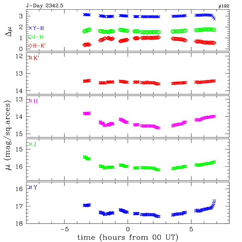
We used archive TNG data taken with the Amici disperser of NICS, the TNG Near Infrared Camera Spectrometer Baffa et al. (2001). These spectra simultaneously cover the 0.9-2.5 $\mu$ m wavelength range at a resolving power R $\simeq 50$ . Although the resolution is by far too low to measure the intensities of the single OH lines, the spectra can be conveniently used to derive the integrated intensities and colours of the airglow within the infrared photometric bands. The results for a typical dark night are displayed in Fig. 5. The emission in the Y (0.97–1.07 $\mu$ m), J (1.17–1.33 $\mu$ m), and H (1.48–1.78 $\mu$ m) photometric bands is dominated by airglow lines, while K’ (1.95–2.30 $\mu$ m) also includes thermal emission from the telescope mirrors. While the temporal variation in the airglow-dominated bands is quite large (up to 1 magnitude), the colours are much more stable, and can be conveniently used to compare with theoretical predictions. The J-H colour is difficult to model, because of the strong contribution of O₂ lines in the J-band (see Sect. 3.4). The Y-H colour, instead, can be accurately modelled because OH accounts for most of the emission in both bands. The airglow in the Y-band is mostly due to OH lines with $\Delta v$ =3 (3–0 and 4–1), while the H-band only contains OH lines with $\Delta v$ =2 (bands from 2–0 to 6–4). Therefore, apart from minor effects related to small temporal variations of the vibrational and rotational temperatures, the Y-H colour should have a quasi-constant value which solely depends on the relative transition probabilities between these vibrational bands. Using the published transition probabilities we expect a photon flux ratio $N_{\lambda}$ (H)/ $N_{\lambda}$ (Y)=10.8, equivalent to a colour Y-H=3.8. The data in Fig. 5 confirm the predicted stability of the Y-H colour but, most important, shows that the airglow emission is 0.8 magnitudes bluer than expected. In other words, the lines in Y band are, on average, a factor of 2 brighter than predicted. This is the same result that we find in the GIANO spectrum.

3.4 O₂ and unidentified lines

The GIANO spectrum includes about 150 lines which cannot be associated to OH transitions. The measured line positions and fluxes are summarised in Table 2. The table lists the observed wavelengths (in vacuum) which are accurate to 0.05 Å r.m.s. The relative photon fluxes and the accuracy flags ( $a$ =best, $c$ =worst) are in the same unit as the OH lines (Sect. 3.1).

All the brightest lines in the J-band are identified as roto-vibrational transitions of the O₂ (0,0) $a^{1}\Delta_{g}-X^{3}\Sigma^{-}_{g}$ band. The observed wavelengths are equal, within the errors, to those listed in the HITRAN database (Rothman et al. (2009)). Most of these lines are coincident with telluric absorption features, i.e. the O₂ lines are optically thick.

The brightest emission features at longer wavelengths are the broad features at 1.5803 and 1.5808 $\mu$ m (see top panel of Fig 6). These features are the band-heads of the (0,1) $a^{1}\Delta_{g}-X^{3}\Sigma^{-}_{g}$ transitions of O₂. This is the first overtone of the (0,0) band discussed above. Most of the lines in the 1.56–1.61 $\mu$ m range are also coincident with O₂ transitions listed in the HITRAN database. Interestingly, none of these emission lines is coincident with telluric absorption features. Therefore, unlike the (0,0) O₂ band, it seems that the (0,1) O₂ lines are optically thin.

The remaining lines are unlikely to be associated to the O₂ band, because they are very far from the O₂ band-heads. An intriguing result is that several of these lines appear as closely spaced doublets with equal intensities (see Fig. 6). In other words, they are very similar to all the $\Lambda$ -split OH doublets detected in our spectra. However, their wavelengths do not correspond to any OH transition with $J_{u}\leq 19.5$ and $v_{u}\leq 10$ . The possibility that these doublets could be produced by OH isotopologues (e.g. ¹⁸OH) should be investigated, but is beyond the aims of this paper.

It is interesting to note that the integrated photon flux due to non-OH lines is about 5% of the total airglow line emission in the H-band. Specifically, about 1.5% is accounted for by the two band-heads around 1.58 $\mu$ m, while the remaining 3.5% is in isolated lines. This contribution is not necessarily negligible and could complicate the design of airglow-subtraction devices for astronomical instruments.

We do not include in the list the broad emission features at wavelengths beyond 2.3 $\mu$ m, which are produced by absorption bands generated at relatively low heights in the atmosphere.

4 Conclusions

Using GIANO at the Telescopio Nazionale Galileo (TNG), we have obtained a high resolution (R $\simeq$ 50,000) flux calibrated spectrum of the night airglow covering the 0.95–2.4 $\mu$ m wavelength range. To the best of our knowledge, this is the first spectrum of this type ever taken.

About 80% of the detected lines can be unambiguously identified as OH transitions. The observed wavelengths agree with those expected by the most accurate molecular energy levels available in the literature (Abrams et al. 1994).

The relative fluxes of OH are used to determine the physical conditions of the emitting molecules. Most of the data are well fitted by a standard model, where the population of the vibrational states follows a Boltzmann distribution at $T_{vib}$ =9000 K, while the rotational levels within a given vibrational state are thermalized at $T_{rot}$ =180 K. However, we also detect lines from highly excited rotational levels. These reveal a population of “hot” OH, with $T_{rot}\simeq T_{vib}$ , which accounts for a few % of the total number of molecules. This result indicates that the time-scales for the thermalization of the rotational levels are not quick enough to completely quench the emission from recently formed molecules in highly excited rotational states.

Most surprisingly, the relative intensities of OH lines from the same upper level show important discrepancies with what predicted by computed transition probabilities.

All the non-OH lines observed in the 1.2-1.3 $\mu$ m range can be identified as O₂ transitions within the (0,0) $a^{1}\Delta_{g}-X^{3}\Sigma^{-}_{g}$ band. The remaining non-OH airglow lines are in the H-band (1.5-1.8 $\mu$ m). Of these, about 2/3 are associated to the first overtone of the same O₂ band, i.e. (0,1) $a^{1}\Delta_{g}-X^{3}\Sigma^{-}_{g}$ at 1.58 $\mu$ m. Interestingly, these lines are not coincident with telluric absorption features, i.e. the lines are, most probably, optically thin. The remaining lines, being far from the O₂ band-heads, are unlikely to be associated to these band.

Acknowledgements.

Part of this work was supported by the grant TECNO-INAF-2011.

References

(1) Abrams, M. C., Davis, S. P., Rao, M. L. P., Engleman, R. Jr., & Brault, J. W. 1994, ApJS, 93, 351
Baffa et al. (2001) Baffa, C., Comoretto, G., Gennari, S., et al. 2001, A&A, 378, 722
(3) Cosby, P. C., Sharpee B. D., Slanger, T. G., Huestis, D. L., & Hanuschik, R. W. 2006, J. Geophys. Res., 111, 2307
(4) Ellis, S. C., Bland-Hawthorn, J., Lawrence, J., et al. 2012, MNRAS, 425, 1682
(5) Hanuschik, R. W. 2003, A&A, 407, 1157
(6) Kaye, J. A. 1988, J. Geophys. Res., 93, 285
(7) Makhlouf, U. B., Picard, R. H., & Winick, R. J. 1995, J. Geophys. Res., 100, 11289
(8) Maihara, T., Iwamuro, F., Yamashita, T., et al. 1993, PASP, 105, 940
(9) Mies, F. H. 1974, J. Mol. Spec., 53, 150
(10) Oliva, E., & Origlia, L. 1992, A&A, 254, 466
(11) Oliva, E., Origlia, L., Maiolino, R., et al. 2012, SPIE, 8446, 3TO
(12) Oliva, E., Biliotti, V., Baffa, C., et al. 2012, SPIE, 8453, 2TO
(13) Osterbrock, D. E., Donald, E., Fulbright, J. P., Cosby, P. C., & Barlow, T. A. 1998, PASP, 110, 1499
(14) Redman, S. L., Lawler, J. E., Nave, G., Ramsey, L. W., & Mahadevan, S. 2011, ApJS, 195, 24
Rothman et al. (2009) Rothman, L. S., Gordon, I. E., Barbe, A., et al. 2009, JQS&RT, 110, 533
(16) Rousselot, P., Lidman, C., Cuby, J.-G., Moreels , G., & Monnet, G. 2000, A&A, 354, 1134 (R2000)
(17) Sharma, R. D. 1985, Handbook of Geophysics, chapter 13 (Air Force Geophysics Laboratory, USAF)
(18) van der Loo, M. P. J., & Groenenboom, G. C. 2007, J. of Chemical Physics, 126, 114314

\LT@array

[x]—r—r—r——r—r—r——r—r—rr— OH line wavelengths and relative photon fluxes
$\lambda_{vac}$ (Å) Iden I¹¹¹¹¹¹ $1$ I is the relative line photons flux. The superscript defines the accuracy ( $a$ =best, $c$ =worst). See text for details. $\lambda_{vac}$ (Å) Iden I¹¹¹¹¹¹ $1$ I is the relative line photons flux. The superscript defines the accuracy ( $a$ =best, $c$ =worst). See text for details. $\lambda_{vac}$ (Å) Iden I¹¹¹¹¹¹ $1$ I is the relative line photons flux. The superscript defines the accuracy ( $a$ =best, $c$ =worst). See text for details.
\endfirstheadcontinued.
$\lambda_{vac}$ (Å) Iden I¹¹¹¹¹¹ $1$ I is the relative line photons flux. The superscript defines the accuracy ( $a$ =best, $c$ =worst). See text for details. $\lambda_{vac}$ (Å) Iden I¹¹¹¹¹¹ $1$ I is the relative line photons flux. The superscript defines the accuracy ( $a$ =best, $c$ =worst). See text for details. $\lambda_{vac}$ (Å) Iden I¹¹¹¹¹¹ $1$ I is the relative line photons flux. The superscript defines the accuracy ( $a$ =best, $c$ =worst). See text for details.
\endhead\endfoot9722.546 [3-0]R1e(1.5) 9740.794 [3-0]R2e(0.5) 9851.125 [3-0]P2e(1.5)
9722.448 [3-0]R1f(1.5) 18^c 9740.726 [3-0]R2f(0.5) 9^c 9851.245 [3-0]P2f(1.5) 16^b
9874.767 [3-0]P1e(2.5) 9897.437 [3-0]P2e(2.5) 9917.249 [3-0]P1e(3.5)
9874.921 [3-0]P1f(2.5) 38^a 9897.479 [3-0]P2f(2.5) 11^c 9917.533 [3-0]P1f(3.5) 41^a
9948.022 [3-0]P2e(3.5) 9959.328 [9-5]R1e(1.5) 9964.447 [3-0]P1e(4.5)
9947.957 [3-0]P2f(3.5) 11^c 9959.286 [9-5]R1f(1.5) 21^b 9964.877 [3-0]P1f(4.5) 23^a
9975.087 [9-5]R2e(0.5) 10002.832 [3-0]P2e(4.5) 10015.583 [9-5]Q1e(1.5)
9975.079 [9-5]R2f(0.5) 6^c 10002.642 [3-0]P2f(4.5) 10^c 10015.527 [9-5]Q1f(1.5) 44^a
10063.407 [9-5]P2e(1.5) 10085.175 [9-5]P1e(2.5) 10106.324 [9-5]P2e(2.5)
10063.538 [9-5]P2f(1.5) 14^b 10085.288 [9-5]P1f(2.5) 38^a 10106.425 [9-5]P2f(2.5) 14^b
10126.670 [9-5]P1e(3.5) 10174.990 [4-1]R1e(3.5) 10183.784 [4-1]R2e(2.5)
10126.898 [9-5]P1f(3.5) 51^a 10174.806 [4-1]R1f(3.5) 19^c 10183.868 [4-1]R2f(2.5) 9^c
10192.575 [4-1]R1e(2.5) 10205.839 [4-1]R2e(1.5) 10211.608 [9-5]P2e(4.5)
10192.425 [4-1]R1f(2.5) 31^a 10205.849 [4-1]R2f(1.5) 12^b 10211.545 [9-5]P2f(4.5) 12^b
10213.900 [4-1]R1e(1.5) 10228.311 [9-5]P1e(5.5) 10233.499 [4-1]R2e(0.5)
10213.802 [4-1]R1f(1.5) 41^a 10228.862 [9-5]P1f(5.5) 12^b 10233.428 [4-1]R2f(0.5) 12^b
10289.505 [4-1]Q1e(1.5) 10299.021 [4-1]Q1e(2.5) 10350.063 [4-1]P2e(1.5)
10289.409 [4-1]Q1f(1.5) 110^a 10298.670 [4-1]Q1f(2.5) 37^a 10350.193 [4-1]P2f(1.5) 23^a
10375.641 [4-1]P1e(2.5) 10399.361 [4-1]P2e(2.5) 10421.071 [4-1]P1e(3.5)
10375.799 [4-1]P1f(2.5) 86^a 10399.413 [4-1]P2f(2.5) 32^a 10421.366 [4-1]P1f(3.5) 92^a
10453.395 [4-1]P2e(3.5) 10471.604 [4-1]P1e(4.5) 10512.107 [4-1]P2e(4.5)
10453.335 [4-1]P2f(3.5) 21^b 10472.056 [4-1]P1f(4.5) 57^a 10511.916 [4-1]P2f(4.5) 11^b
10527.345 [4-1]P1e(5.5) 10700.140 [5-2]R1e(4.5) 10713.770 [5-2]R1e(3.5)
10527.969 [4-1]P1f(5.5) 29^a 10699.948 [5-2]R1f(4.5) 7^c 10713.589 [5-2]R1f(3.5) 22^a
10723.304 [5-2]R2e(2.5) 10731.788 [5-2]R1e(2.5) 10746.145 [5-2]R2e(1.5)
10723.396 [5-2]R2f(2.5) 10^b 10731.640 [5-2]R1f(2.5) 45^a 10746.159 [5-2]R2f(1.5) 16^a
10753.969 [5-2]R1e(1.5) 10775.094 [5-2]R2e(0.5) 10832.411 [5-2]Q2e(0.5)
10753.871 [5-2]R1f(1.5) 56^a 10775.024 [5-2]R2f(0.5) 12^b 10832.103 [5-2]Q2f(0.5) 15^b
10834.338 [5-2]Q1e(1.5) 10844.871 [5-2]Q1e(2.5) 10860.033 [5-2]Q1e(3.5)
10834.241 [5-2]Q1f(1.5) 161^b 10844.514 [5-2]Q1f(2.5) 56^a 10859.222 [5-2]Q1f(3.5) 15^a
10898.609 [5-2]P2e(1.5) 10926.348 [5-2]P1e(2.5) 10951.316 [5-2]P2e(2.5)
10898.751 [5-2]P2f(1.5) 31^b 10926.511 [5-2]P1f(2.5) 115^a 10951.381 [5-2]P2f(2.5) 39^a
10975.177 [5-2]P1e(3.5) 11009.318 [5-2]P2e(3.5) 11029.577 [5-2]P1e(4.5)
10975.484 [5-2]P1f(3.5) 120^b 11009.269 [5-2]P2f(3.5) 26^b 11030.053 [5-2]P1f(4.5) 72^b
11072.551 [5-2]P2e(4.5) 11089.688 [5-2]P1e(5.5) 11312.937 [6-3]R1e(3.5)
11072.363 [5-2]P2f(4.5) 12^b 11090.349 [5-2]P1f(5.5) 33^a 11312.764 [6-3]R1f(3.5) 26^c
11323.318 [6-3]R2e(2.5) 11331.266 [6-3]R1e(2.5) 11439.989 [6-3]Q1e(1.5)
11323.415 [6-3]R2f(2.5) 14^c 11331.121 [6-3]R1f(2.5) 42^c 11439.891 [6-3]Q1f(1.5) 124^b
11451.787 [6-3]Q1e(2.5) 11538.706 [6-3]P1e(2.5) 11591.523 [6-3]P1e(3.5)
11451.422 [6-3]Q1f(2.5) 39^b 11538.876 [6-3]P1f(2.5) 93^c 11591.847 [6-3]P1f(3.5) 91^b
11627.867 [6-3]P2e(3.5) 11650.492 [6-3]P1e(4.5) 11696.442 [6-3]P2e(4.5)
11627.826 [6-3]P2f(3.5) 32^b 11651.000 [6-3]P1f(4.5) 61^c 11696.254 [6-3]P2f(4.5) 18^b
11715.795 [6-3]P1e(5.5) 11771.004 [6-3]P2e(5.5) 11787.563 [6-3]P1e(6.5)
11716.506 [6-3]P1f(5.5) 36^a 11770.650 [6-3]P2f(5.5) 6^c 11788.495 [6-3]P1f(6.5) 14^b
11983.237 [7-4]R2e(3.5) 11988.729 [7-4]R1e(3.5) 12000.086 [7-4]R2e(2.5)
11983.411 [7-4]R2f(3.5) 5^a 11988.565 [7-4]R1f(3.5) 26^b 12000.197 [7-4]R2f(2.5) 14^a
12007.149 [7-4]R1e(2.5) 12024.233 [7-4]R2e(1.5) 12030.932 [7-4]R1e(1.5)
12007.008 [7-4]R1f(2.5) 56^a 12024.259 [7-4]R2f(1.5) 21^a 12030.837 [7-4]R1f(1.5) 62^b
12055.912 [7-4]R2e(0.5) 12120.556 [7-4]Q2e(0.5) 12122.690 [7-4]Q1e(1.5)
12055.843 [7-4]R2f(0.5) 22^a 12120.218 [7-4]Q2f(0.5) 12^a 12122.591 [7-4]Q1f(1.5) 166^a
12136.107 [7-4]Q1e(2.5) 12155.358 [7-4]Q1e(3.5) 12196.299 [7-4]P2e(1.5)
12135.738 [7-4]Q1f(2.5) 62^a 12154.512 [7-4]Q1f(3.5) 13^b 12196.471 [7-4]P2f(1.5) 37^a
12229.206 [7-4]P1e(2.5) 12257.680 [7-4]P2e(2.5) 12286.820 [7-4]P1e(3.5)
12229.381 [7-4]P1f(2.5) 142^a 12257.777 [7-4]P2f(2.5) 53^a 12287.159 [7-4]P1f(3.5) 157^a
12325.925 [7-4]P2e(3.5) 12351.329 [7-4]P1e(4.5) 12400.967 [7-4]P2e(4.5)
12325.901 [7-4]P2f(3.5) 41^a 12351.866 [7-4]P1f(4.5) 102^a 12400.789 [7-4]P2f(4.5) 24^a
12422.967 [7-4]P1e(5.5) 12482.885 [7-4]P2e(5.5) 12501.915 [7-4]P1e(6.5)
12423.727 [7-4]P1f(5.5) 52^a 12482.530 [7-4]P2f(5.5) 13^a 12502.919 [7-4]P1f(6.5) 19^a
12571.855 [7-4]P2e(6.5) 12588.345 [7-4]P1e(7.5) 12748.001 [8-5]R1e(5.5)
12571.304 [7-4]P2f(6.5) 5^a 12589.613 [7-4]P1f(7.5) 8^a 12747.917 [8-5]R1f(5.5) 11^a
12752.864 [8-5]R1e(4.5) 12760.892 [8-5]R2e(3.5) 12764.492 [8-5]R1e(3.5)
12752.732 [8-5]R1f(4.5) 31^a 12761.093 [8-5]R2f(3.5) 10^a 12764.343 [8-5]R1f(3.5) 179^c
12777.032 [8-5]R2e(2.5) 12782.634 [8-5]R1e(2.5) 12801.522 [8-5]R2e(1.5)
12777.167 [8-5]R2f(2.5) 22^a 12782.500 [8-5]R1f(2.5) 165^c 12801.565 [8-5]R2f(1.5) 31^a
12807.030 [8-5]R1e(1.5) 12834.593 [8-5]R2e(0.5) 12903.707 [8-5]Q2e(0.5)
12806.937 [8-5]R1f(1.5) 120^c 12834.535 [8-5]R2f(0.5) 34^a 12903.358 [8-5]Q2f(0.5) 23^a
12905.761 [8-5]Q1e(1.5) 12921.319 [8-5]Q1e(2.5) 12943.607 [8-5]Q1e(3.5)
12905.661 [8-5]Q1f(1.5) 256^a 12920.945 [8-5]Q1f(2.5) 77^a 12942.746 [8-5]Q1f(3.5) 26^a
12985.550 [8-5]P2e(1.5) 13021.544 [8-5]P1e(2.5) 13052.678 [8-5]P2e(2.5)
12985.742 [8-5]P2f(1.5) 53^a 13021.726 [8-5]P1f(2.5) 188^a 13052.801 [8-5]P2f(2.5) 71^a
13085.086 [8-5]P1e(3.5) 13127.821 [8-5]P2e(3.5) 13156.506 [8-5]P1e(4.5)
13085.443 [8-5]P1f(3.5) 206^a 13127.823 [8-5]P2f(3.5) 59^b 13157.079 [8-5]P1f(4.5) 64^b
13210.926 [8-5]P2e(4.5) 13236.106 [8-5]P1e(5.5) 14833.285 [3-1]R1e(2.5)
13210.769 [8-5]P2f(4.5) 31^b 13236.927 [8-5]P1f(5.5) 88^b 14832.903 [3-1]R1f(2.5) 205^c
14864.398 [3-1]R2e(1.5) 14886.507 [2-0]P2e(5.5) 14887.819 [3-1]R1e(1.5)
14864.398 [3-1]R2f(1.5) 59^c 14885.824 [2-0]P2f(5.5) 12^c 14887.579 [3-1]R1f(1.5) 276^c
14908.278 [2-0]P1e(6.5) 14931.971 [3-1]R2e(0.5) 15025.142 [2-0]P1e(7.5)
14909.776 [2-0]P1f(6.5) 32^c 14931.795 [3-1]R2f(0.5) 114^c 15026.969 [2-0]P1f(7.5) 5^c
15053.190 [3-1]Q2e(0.5) 15055.657 [3-1]Q1e(1.5) 15064.542 [3-1]Q2e(1.5)
15052.540 [3-1]Q2f(0.5) 80^b 15055.442 [3-1]Q1f(1.5) 841^a 15063.455 [3-1]Q2f(1.5) 25^a
15069.360 [3-1]Q1e(2.5) 15082.841 [3-1]Q2e(2.5) 15089.161 [3-1]Q1e(3.5)
15068.575 [3-1]Q1f(2.5) 274^a 15081.669 [3-1]Q2f(2.5) 6^c 15087.391 [3-1]Q1f(3.5) 63^c
15107.805 [3-1]Q2e(3.5) 15115.312 [3-1]Q1e(4.5) 15187.009 [3-1]P2e(1.5)
15106.959 [3-1]Q2f(3.5) 4^a 15112.139 [3-1]Q1f(4.5) 16^b 15187.271 [3-1]P2f(1.5) 158^b
15240.788 [3-1]P1e(2.5) 15287.747 [3-1]P2e(2.5) 15332.099 [3-1]P1e(3.5)
15241.120 [3-1]P1f(2.5) 712^b 15287.831 [3-1]P2f(2.5) 203^b 15332.705 [3-1]P1f(3.5) 729^b
15395.411 [3-1]P2e(3.5) 15431.702 [3-1]P1e(4.5) 15462.443 [4-2]R1e(5.5)
15395.258 [3-1]P2f(3.5) 153^b 15432.613 [3-1]P1f(4.5) 406^b 15461.807 [4-2]R1f(5.5) 11^b
15473.986 [4-2]R2e(4.5) 15501.158 [4-2]R1e(4.5) 15509.979 [3-1]P2e(4.5)
15474.439 [4-2]R2f(4.5) 8^b 15500.571 [4-2]R1f(4.5) 44^b 15509.559 [3-1]P2f(4.5) 84^b
15517.706 [4-2]R2e(3.5) 15539.711 [3-1]P1e(5.5) 15546.392 [4-2]R1e(3.5)
15518.039 [4-2]R2f(3.5) 26^b 15540.945 [3-1]P1f(5.5) 198^b 15545.890 [4-2]R1f(3.5) 123^b
15570.070 [4-2]R2e(2.5) 15597.824 [4-2]R1e(2.5) 15631.677 [3-1]P2e(5.5)
15570.249 [4-2]R2f(2.5) 61^b 15597.439 [4-2]R1f(2.5) 263^b 15630.972 [3-1]P2f(5.5) 67^c
15631.562 [4-2]R2e(1.5) 15655.074 [4-2]R1e(1.5) 15656.177 [3-1]P1e(6.5)
15631.560 [4-2]R2f(1.5) 67^c 15654.833 [4-2]R1f(1.5) 343^a 15657.749 [3-1]P1f(6.5) 61^a
15702.631 [4-2]R2e(0.5) 15760.831 [3-1]P2e(6.5) 15781.163 [3-1]P1e(7.5)
15702.447 [4-2]R2f(0.5) 96^b 15759.827 [3-1]P2f(6.5) 9^b 15783.090 [3-1]P1f(7.5) 15^a
15830.675 [4-2]Q2e(0.5) 15833.381 [4-2]Q1e(1.5) 15843.076 [4-2]Q2e(1.5)
15829.995 [4-2]Q2f(0.5) 89^a 15833.165 [4-2]Q1f(1.5) 1000^a 15841.930 [4-2]Q2f(1.5) 35^a
15848.459 [4-2]Q1e(2.5) 15863.115 [4-2]Q2e(2.5) 15870.210 [4-2]Q1e(3.5)
15847.662 [4-2]Q1f(2.5) 325^a 15861.863 [4-2]Q2f(2.5) 10^a 15868.404 [4-2]Q1f(3.5) 93^a
15897.794 [3-1]P2e(7.5) 15898.914 [4-2]Q1e(4.5) 15914.773 [3-1]P1e(8.5)
15896.476 [3-1]P2f(7.5) 12^b 15895.662 [4-2]Q1f(4.5) 16^b 15917.072 [3-1]P1f(8.5) 5^b
15972.456 [4-2]P2e(1.5) 16030.661 [4-2]P1e(2.5) 16057.155 [3-1]P1e(9.5)
15972.738 [4-2]P2f(1.5) 217^a 16031.002 [4-2]P1f(2.5) 759^a 16059.850 [3-1]P1f(9.5) 7^a
16079.701 [4-2]P2e(2.5) 16128.294 [4-2]P1e(3.5) 16194.686 [4-2]P2e(3.5)
16079.804 [4-2]P2f(2.5) 262^a 16128.923 [4-2]P1f(3.5) 799^a 16194.544 [4-2]P2f(3.5) 193^a
16234.899 [4-2]P1e(4.5) 16246.367 [5-3]R1e(7.5) 16252.431 [5-3]R2e(6.5)
16235.854 [4-2]P1f(4.5) 500^a 16245.772 [5-3]R1f(7.5) 7^b 16253.038 [5-3]R2f(6.5) 4^b
16270.627 [5-3]R1e(6.5) 16279.449 [5-3]R2e(5.5) 16302.584 [5-3]R1e(5.5)
16270.010 [5-3]R1f(6.5) 11^b 16280.005 [5-3]R2f(5.5) 4^b 16301.973 [5-3]R1f(5.5) 15^b
16315.279 [5-3]R2e(4.5) 16317.374 [4-2]P2e(4.5) 16342.041 [5-3]R1e(4.5)
16315.752 [5-3]R2f(4.5) 9^a 16316.949 [4-2]P2f(4.5) 96^a 16341.470 [5-3]R1f(4.5) 41^a
16350.651 [4-2]P1e(5.5) 16359.060 [3-1]P2e(10.5) 16360.209 [5-3]R2e(3.5)
16351.954 [4-2]P1f(5.5) 207^a 16356.690 [3-1]P2f(10.5) 6^b 16360.561 [5-3]R2f(3.5) 21^a

16369.059 [3-1]P1e(11.5) 16388.740 [5-3]R1e(3.5) 16414.641 [5-3]R2e(2.5)
16372.618 [3-1]P1f(11.5) 7^a 16388.245 [5-3]R1f(3.5) 117^a 16414.835 [5-3]R2f(2.5) 50^a
16442.346 [5-3]R1e(2.5) 16447.981 [4-2]P2e(5.5) 16475.648 [4-2]P1e(6.5)
16441.964 [5-3]R1f(2.5) 245^a 16447.253 [4-2]P2f(5.5) 39^a 16477.319 [4-2]P1f(6.5) 80^a
16479.059 [5-3]R2e(1.5) 16502.485 [5-3]R1e(1.5) 16553.907 [5-3]R2e(0.5)
16479.065 [5-3]R2f(1.5) 93^a 16502.245 [5-3]R1f(1.5) 327^a 16553.723 [5-3]R2f(0.5) 107^a
16586.848 [4-2]P2e(6.5) 16609.994 [4-2]P1e(7.5) 16689.558 [5-3]Q2e(0.5)
16585.798 [4-2]P2f(6.5) 15^a 16612.052 [4-2]P1f(7.5) 25^b 16688.846 [5-3]Q2f(0.5) 84^b
16692.490 [5-3]Q1e(1.5) 16703.242 [5-3]Q2e(1.5) 16709.258 [5-3]Q1e(2.5)
16692.270 [5-3]Q1f(1.5) 854^a 16702.035 [5-3]Q2f(1.5) 23^a 16708.445 [5-3]Q1f(2.5) 290^a
16718.914 [3-1]P1e(13.5) 16725.407 [5-3]Q2e(2.5) 16733.405 [5-3]Q1e(3.5)
16723.436 [3-1]P1f(13.5) 10^a 16724.073 [5-3]Q2f(2.5) 5^b 16731.555 [5-3]Q1f(3.5) 81^b
16734.354 [4-2]P2e(7.5) 16753.832 [4-2]P1e(8.5) 16755.756 [5-3]Q2e(3.5)
16732.965 [4-2]P2f(7.5) 9^b 16756.299 [4-2]P1f(8.5) 3^b 16754.736 [5-3]Q2f(3.5) 10^b
16765.246 [5-3]Q1e(4.5) 16840.325 [5-3]P2e(1.5) 16890.892 [4-2]P2e(8.5)
16761.899 [5-3]Q1f(4.5) 23^a 16840.636 [5-3]P2f(1.5) 116^a 16889.145 [4-2]P2f(8.5) 8^a
16903.502 [5-3]P1e(2.5) 16907.350 [4-2]P1e(9.5) 16908.877 [3-1]P1e(14.5)
16903.857 [5-3]P1f(2.5) 687^a 16910.250 [4-2]P1f(9.5) 13^b 16913.912 [3-1]P1f(14.5) 10^a
16955.012 [5-3]P2e(2.5) 17008.426 [5-3]P1e(3.5) 17056.858 [4-2]P2e(9.5)
16955.145 [5-3]P2f(2.5) 238^a 17009.087 [5-3]P1f(3.5) 692^a 17054.733 [4-2]P2f(9.5) 6^b
17070.789 [4-2]P1e(10.5) 17078.430 [5-3]P2e(3.5) 17109.370 [3-1]P1e(15.5)
17074.147 [4-2]P1f(10.5) 9^a 17078.309 [5-3]P2f(3.5) 173^a 17114.928 [3-1]P1f(15.5) 9^a
17123.152 [5-3]P1e(4.5) 17175.355 [6-4]R1e(8.5) 17189.235 [6-4]R1e(7.5)
17124.166 [5-3]P1f(4.5) 445^a 17174.899 [6-4]R1f(8.5) 7^b 17188.696 [6-4]R1f(7.5) 9^b
17210.529 [5-3]P2e(4.5) 17211.958 [6-4]R1e(6.5) 17243.338 [6-4]R1e(5.5)
17210.109 [5-3]P2f(4.5) 87^a 17211.371 [6-4]R1f(6.5) 6^a 17242.741 [6-4]R1f(5.5) 15^b
17247.926 [5-3]P1e(5.5) 17257.360 [6-4]R2e(4.5) 17283.151 [6-4]R1e(4.5)
17249.321 [5-3]P1f(5.5) 205^b 17257.853 [6-4]R2f(4.5) 13^b 17282.584 [6-4]R1f(4.5) 44^a
17303.187 [6-4]R2e(3.5) 17331.117 [6-4]R1e(3.5) 17351.525 [5-3]P2e(5.5)
17303.553 [6-4]R2f(3.5) 21^a 17330.621 [6-4]R1f(3.5) 10^b 17350.779 [5-3]P2f(5.5) 42^b
17359.587 [6-4]R2e(2.5) 17382.907 [5-3]P1e(6.5) 17386.887 [6-4]R1e(2.5)
17359.787 [6-4]R2f(2.5) 47^b 17384.705 [5-3]P1f(6.5) 80^b 17386.504 [6-4]R1f(2.5) 214^b
17418.706 [4-2]P2e(11.5) 17427.043 [6-4]R2e(1.5) 17428.610 [4-2]P1e(12.5)
17415.758 [4-2]P2f(11.5) 5^a 17427.047 [6-4]R2f(1.5) 85^a 17432.965 [4-2]P1f(12.5) 10^a
17450.087 [6-4]R1e(1.5) 17501.775 [5-3]P2e(6.5) 17505.994 [6-4]R2e(0.5)
17449.846 [6-4]R1f(1.5) 244^a 17500.681 [5-3]P2f(6.5) 16^a 17505.801 [6-4]R2f(0.5) 85^a
17528.254 [5-3]P1e(7.5) 17541.515 [3-1]P2e(16.5) 17543.701 [3-1]P1e(17.5)
17530.474 [5-3]P1f(7.5) 26^a 17536.573 [3-1]P2f(16.5) 5^a 17550.297 [3-1]P1f(17.5) 7^a
17650.227 [6-4]Q2e(0.5) 17653.333 [6-4]Q1e(1.5) 17665.519 [6-4]Q2e(1.5)
17649.480 [6-4]Q2f(0.5) 68^a 17653.111 [6-4]Q1f(1.5) 622^a 17664.243 [6-4]Q2f(1.5) 19^b
17672.224 [6-4]Q1e(2.5) 17684.161 [5-3]P1e(8.5) 17690.349 [6-4]Q2e(2.5)
17671.400 [6-4]Q1f(2.5) 196^a 17686.826 [5-3]P1f(8.5) 12^a 17688.922 [6-4]Q2f(2.5) 8^a
17699.386 [6-4]Q1e(3.5) 17724.421 [6-4]Q2e(3.5) 17735.169 [6-4]Q1e(4.5)
17697.499 [6-4]Q1f(3.5) 31^c 17723.298 [6-4]Q2f(3.5) 3^b 17731.742 [6-4]Q1f(4.5) 11^b
17779.850 [6-4]Q1e(5.5) 17811.307 [6-4]P2e(1.5) 17823.338 [4-2]P2e(13.5)
17774.412 [6-4]Q1f(5.5) 6^a 17811.642 [6-4]P2f(1.5) 15^c 17819.490 [4-2]P2f(13.5) 6^a
17831.728 [5-3]P2e(8.5) 17830.122 [4-2]P1e(14.5) 17850.874 [5-3]P1e(9.5)
17829.880 [5-3]P2f(8.5) 9^a 17835.564 [4-2]P1f(14.5) 7^a 17854.007 [5-3]P1f(9.5) 6^c
17880.118 [6-4]P1e(2.5) 17993.620 [6-4]P1e(3.5) 18067.987 [6-4]P2e(3.5)
17880.481 [6-4]P1f(2.5) 456^b 17994.304 [6-4]P1f(3.5) 382^c 18067.882 [6-4]P2f(3.5) 28^c
19560.004 [7-5]P1e(6.5) 19618.495 [8-6]R2e(3.5) 19642.698 [8-6]R1e(3.5)
19562.060 [7-5]P1f(6.5) 21^c 19618.954 [8-6]R2f(3.5) 17^c 19642.237 [8-6]R1f(3.5) 49^c
19677.859 [8-6]R2e(2.5) 19699.527 [7-5]P2e(6.5) 19702.267 [8-6]R1e(2.5)
19678.136 [8-6]R2f(2.5) 18^c 19698.347 [7-5]P2f(6.5) 14^c 19701.898 [8-6]R1f(2.5) 84^c
19734.919 [7-5]P1e(7.5) 19751.486 [8-6]R2e(1.5) 19771.980 [8-6]R1e(1.5)
19737.499 [7-5]P1f(7.5) 33^c 19751.543 [8-6]R2f(1.5) 100^c 19771.744 [8-6]R1f(1.5) 137^c
19774.061 [6-4]P1e(13.5) 19839.814 [8-6]R2e(0.5) 20005.417 [8-6]Q2e(0.5)
19780.072 [6-4]P1f(13.5) 8^c 19839.643 [8-6]R2f(0.5) 54^c 20004.611 [8-6]Q2f(0.5) 21^c

20008.276 [8-6]Q1e(1.5) 20033.634 [8-6]Q1e(2.5) 20069.974 [8-6]Q1e(3.5)
20008.051 [8-6]Q1f(1.5) 280^c 20032.788 [8-6]Q1f(2.5) 72^c 20068.017 [8-6]Q1f(3.5) 10^c
20193.020 [8-6]P2e(1.5) 20275.646 [8-6]P1e(2.5) 20320.599 [7-5]P2e(9.5)
20193.434 [8-6]P2f(1.5) 43^c 20276.033 [8-6]P1f(2.5) 241^c 20318.028 [7-5]P2f(9.5) 7^a
20339.372 [8-6]P2e(2.5) 20343.553 [7-5]P1e(10.5) 20412.304 [8-6]P1e(3.5)
20339.623 [8-6]P2f(2.5) 110^b 20347.960 [7-5]P1f(10.5) 9^a 20413.054 [8-6]P1f(3.5) 41^c
20499.371 [8-6]P2e(3.5) 20562.953 [8-6]P1e(4.5) 20673.021 [8-6]P2e(4.5)
20499.358 [8-6]P2f(3.5) 0^c 20564.143 [8-6]P1f(4.5) 219^c 20672.668 [8-6]P2f(4.5) 14^c
20728.171 [8-6]P1e(5.5) 20807.364 [7-5]P2e(11.5) 20824.588 [7-5]P1e(12.5)
20729.859 [8-6]P1f(5.5) 135^c 20803.671 [7-5]P2f(11.5) 5^a 20830.495 [7-5]P1f(12.5) 12^b
20860.621 [8-6]P2e(5.5) 20875.692 [6-4]P1e(17.5) 20908.450 [8-6]P1e(6.5)
20859.871 [8-6]P2f(5.5) 34^b 20885.483 [6-4]P1f(17.5) 6^a 20910.685 [8-6]P1f(6.5) 65^b
21089.760 [7-5]P1e(13.5) 21096.316 [9-7]R2e(3.5) 21104.276 [8-6]P1e(7.5)
21096.527 [7-5]P1f(13.5) 10^b 21096.889 [9-7]R2f(3.5) 8^b 21107.104 [8-6]P1f(7.5) 27^b
21116.060 [9-7]R1e(3.5) 21155.925 [9-7]R2e(2.5) 21176.727 [9-7]R1e(2.5)
21115.653 [9-7]R1f(3.5) 49^b 21156.307 [9-7]R2f(2.5) 20^a 21176.387 [9-7]R1f(2.5) 70^a
21194.919 [6-4]P1e(18.5) 21232.354 [9-7]R2e(1.5) 21249.706 [9-7]R1e(1.5)
21205.938 [6-4]P1f(18.5) 5^c 21232.494 [9-7]R2f(1.5) 30^a 21249.481 [9-7]R1f(1.5) 95^a
21279.892 [8-6]P2e(7.5) 21316.180 [8-6]P1e(8.5) 21326.033 [9-7]R2e(0.5)
21278.218 [8-6]P2f(7.5) 16^a 21319.652 [8-6]P1f(8.5) 18^a 21325.914 [9-7]R2f(0.5) 26^a
21372.519 [7-5]P1e(14.5) 21505.452 [9-7]Q2e(0.5) 21507.422 [9-7]Q1e(1.5)
21380.238 [7-5]P1f(14.5) 9^a 21504.638 [9-7]Q2f(0.5) 20^a 21507.196 [9-7]Q1f(1.5) 211^a
21513.007 [8-6]P2e(8.5) 21537.948 [9-7]Q1e(2.5) 21710.932 [9-7]P2e(1.5)
21510.804 [8-6]P2f(8.5) 5^a 21537.098 [9-7]Q1f(2.5) 85^b 21711.408 [9-7]P2f(1.5) 52^a
21790.783 [8-6]P1e(10.5) 21802.112 [9-7]P1e(2.5) 21873.347 [9-7]P2e(2.5)
21795.718 [8-6]P1f(10.5) 7^b 21802.515 [9-7]P1f(2.5) 168^a 21873.690 [9-7]P2f(2.5) 66^a
21955.240 [9-7]P1e(3.5) 22052.320 [9-7]P2e(3.5) 22124.874 [9-7]P1e(4.5)
21956.036 [9-7]P1f(3.5) 190^a 22052.412 [9-7]P2f(3.5) 60^a 22126.160 [9-7]P1f(4.5) 158^a
22311.800 [9-7]P1e(5.5) 22460.602 [9-7]P2e(5.5) 22516.726 [9-7]P1e(6.5)
22313.651 [9-7]P1f(5.5) 78^a 22459.926 [9-7]P2f(5.5) 24^a 22519.211 [9-7]P1f(6.5) 40^a
22690.982 [9-7]P2e(6.5) 22740.375 [9-7]P1e(7.5)
22689.823 [9-7]P2f(6.5) 9^c 22743.555 [9-7]P1f(7.5) 20^c
³³3

Table 2: Observed wavelengths and relative photon fluxes of other airglow lines

$\lambda_{vac}$ (Å)	Iden¹¹¹¹¹¹ $1$ Identification based on the HITRAN database.	I²²²²²² $2$ I is the relative line photons flux. The superscript defines the accuracy ( $a$ =best, $c$ =worst). See text for details.	$\lambda_{vac}$ (Å)	Iden¹¹¹¹¹¹ $1$ Identification based on the HITRAN database.	I²²²²²² $2$ I is the relative line photons flux. The superscript defines the accuracy ( $a$ =best, $c$ =worst). See text for details.	$\lambda_{vac}$ (Å)	Iden¹¹¹¹¹¹ $1$ Identification based on the HITRAN database.	I²²²²²² $2$ I is the relative line photons flux. The superscript defines the accuracy ( $a$ =best, $c$ =worst). See text for details.
12496.20	O₂	8^a	12511.21	O₂	12^a	12526.55	O₂	28^a
12542.18	O₂	32^b	12558.15	O₂	34^b	12574.44	O₂	28^b
12586.61	O₂	5^b	12591.02	O₂	21^b	12592.36	O₂	9^a
12594.06	O₂	3^b	12595.79	O₂	8^a	12598.38	O₂	15^b
12601.82	O₂	21^b	12604.71	O₂	23^b	12608.04	O₂	46^b
12611.33	O₂	33^b	12614.69	O₂	31^b	12618.21	O₂	32^b
12621.57	O₂	25^b	12625.29	O₂	42^b	12628.67	O₂	12^b
12632.84	O₂	11^b	12636.11	O₂	3^c	12640.60	O₂	13^b
12642.75	O₂	36^b	12648.58	O₂	10^c	12651.77	O₂	8^c
12656.85	O₂	14^b	12660.70	O₂	56^b	12665.46	O₂	39^b
12674.38	O₂	12^b	12677.40	O₂	10^b	12683.66	O₂	20^b
12684.19	O₂	74^b	12685.04	O₂	96^b	12686.11	O₂	13^b
12686.85	O₂	21^b	12687.58	O₂	37^b	12688.99	O₂	10^b
12691.16	O₂	10^b	12692.90	O₂	63^b	12693.31	O₂	63^b
12694.21	¹⁶O¹⁸O	19^c	12695.27	O₂	39^c	12695.72	O₂	41^c
12696.28	O₂	38^c	12697.20	O₂	16^a	12697.86	O₂	11^b
12698.62	O₂	73^b	12700.58	O₂	16^a	12701.34	O₂	44^a
12704.27	O₂	26^a	12707.05	O₂	80^b	12710.31	O₂	11^b
12717.13	O₂	32^b	12720.32	O₂	75^b	12725.41	O₂	13^b
12727.44	O₂	27^b	12730.59	O₂	60^b	12738.01	O₂	36^b
12741.12	O₂	62^b	12744.70	O₂	15^b	12748.83	O₂	52^b
12751.93	O₂	73^b	12759.93	O₂	77^b	12762.99	O₂	85^b
12764.29	O₂	19^b	12771.29	O₂	76^b	12774.32	O₂	85^b
12782.76	O₂	14^b	12784.13	O₂	14^b	12785.94	O₂	66^b
12794.85	O₂	46^b	12797.84	O₂	43^b	12804.29	O₂	14^b
12807.01	O₂	11^a	12809.98	O₂	23^a	12819.49	O₂	13^b
12822.42	O₂	13^b	12824.77	O₂	14^a	12845.55	O₂	10^b
12866.60	O₂	65^a	12888.05	O₂	39^a	12909.80	O₂	25^a
12931.85	O₂	7^a	15310.63		6^a	15348.59		16^a
15488.78		9^a	15542.68		5^b	15601.79	O₂	4^b
15612.60	doublet?	3^b	15613.90	doublet?	3^b	15628.91	O₂	5^a
15666.07		3^c	15671.44		2^c	15679.25		2^c
15683.69	O₂	11^a	15692.47	O₂	4^b	15697.67	O₂	5^b
15705.84	O₂	7^b	15711.43	O₂	16^b	15719.34	O₂	10^b
15724.47	O₂	13^b	15732.97	O₂	14^b	15738.05	O₂	18^b
15739.41	O₂	12^b	15746.73	O₂	16^b	15751.78	O₂	21^b
15760.69	O₂	21^b	15765.61	O₂	24^b	15767.71	O₂	12^b
15774.70	O₂	14^b	15779.60	O₂	26^b	15788.95		6^b
15793.69	O₂	26^b	15803.00	O₂ Band-head	99^a	15808.00	O₂ Band-head	178^a
15823.83		8^b	15838.42	O₂	16^b	15853.03	O₂	17^a
15858.01	O₂	13^a	15867.73	O₂	12^a	15872.65	O₂	15^a
15874.97		6^b	15882.48	O₂	16^a	15887.36	O₂	13^a
15902.13	O₂	10^a	15912.28	O₂	9^a	15925.01		10^a
15927.31		4^a	15929.70		4^a	15932.03		4^a
15934.81		3^a	15954.28		8^a	15983.64		5^a
16013.25		3^c	16073.82		4^c	16097.55		4^c
16118.81		6^b	16159.11		18^b	16208.13		5^b
16220.87		9^a	16228.48	Broad	8^b	16307.46	doublet?	8^a
16308.19	doublet?	8^a	16363.86	doublet?	5^a	16364.93	doublet?	5^a
16438.93	doublet?	3^a	16440.40	doublet?	3^a	17013.19		5^a
17057.13		15^a	17274.51	doublet?	6^a	17275.67	doublet?	6^a

⁴⁴4